Article

Exceptional Drought across Southeastern Australia Caused by Extreme Lack of Precipitation and Its Impacts on NDVI and SIF in 2018

1
Faculty of Geographical Science, Beijing Normal University, Beijing 100875, China
2
State Key Laboratory of Remote Sensing Science, Beijing Normal University, Beijing 100875, China
3
Beijing Key Laboratory for Remote Sensing of Environment and Digital Cities, Beijing 100875, China
4
Faculty of Science, University of Technology Sydney, Sydney 2007, Australia
*
Author to whom correspondence should be addressed.
Remote Sens. 2020, 12(1), 54; https://doi.org/10.3390/rs12010054
Submission received: 19 November 2019 / Revised: 15 December 2019 / Accepted: 19 December 2019 / Published: 21 December 2019

Abstract

:
Increased drought frequency in Australia is a pressing concern for scholars. In 2018, a severe drought in eastern Australia was recorded by the Emergency Events Database (EM-DAT). To investigate the main causes and impacts of this drought across southeastern Australia, this work presents an overview of the drought mechanism and depicts its evolutionary process. The Standardized Precipitation Evapotranspiration Index (SPEI) from the Global Drought Monitor was used to identify the drought event and characterize its spatiotemporal distribution. The Normalized Difference Vegetation Index (NDVI) and the sun-induced chlorophyll fluorescence (SIF) were used to investigate the drought impacts on vegetation growth. In addition, the effects of drought response measures on Sustainable Development Goals (SDGs) were analyzed. Our results showed that the exceptional drought occurred across southeastern Australia from April to December, and it was most severe in July, owing to an extreme lack of precipitation and increase in temperature. Moreover, we identified profound and long-lasting impacts of the drought on NDVI and SIF levels, especially for cropland. Furthermore, we also found that SIF was superior to NDVI in detecting drought impacts. This study advised on how to formulate timely and effective drought-response measures and supports sustainable socioeconomic development in Australia.

Graphical Abstract

1. Introduction

Global warming is an irreversible trend [1,2,3], and as a result, extreme climate events (such as EI Niño and La Niña events) frequently occur in most parts of the world and contribute to climate-driven and water-related hazards, such as droughts [4,5]. Unlike other weather-related hazards (such as windstorms, high temperatures, and chilling damage), drought is the result of the interaction of multiple aspects, which would increase the uncertainty of drought prediction [6,7]. Drought frequency, duration, and severity are expected to increase because of climate change, and the spatial distribution of drought at the global scale indicates that dry zones will become even drier [8,9,10]. This is a long-term threat to sustainable socioeconomic development, and its consequences include crop failure, starvation, and death [11].
Drought is considered to be the costliest natural hazard worldwide, with a recurring feature in most climatic zones [12,13]. It is closely correlated with regional meteorological conditions. For example, abnormal warming and an extreme lack of precipitation greatly contribute to drought, and they are simultaneously accompanied by a sharp decrease in surface evapotranspiration and soil moisture [14,15]. Moreover, drought is also correlated with regional environmental conditions. For example, an increasingly aggravated drought situation (measured by drought frequency, duration, and intensity) in east Africa was primarily caused by a sudden drop in precipitation and water storage [16]. Temperature has been the dominant meteorological cause of drought in semi-arid regions, while precipitation deficiencies have led to drought in tropical savanna climatic zones in Nigeria [17].
Drought is also an agricultural and socioeconomic-related concept [18]. A drought can severely impact vegetation growth and reduce total surface runoff and groundwater storage. A sustained drought can lead to a decrease in surface water, which is crucial for irrigation [19]. Correspondingly, it can threaten the economy, employment, food security, and industrial trade [20,21,22]. Vegetation greenness indices—such as the Normalized Difference Vegetation Index (NDVI) and the Enhanced Vegetation Index (EVI)—have been widely used to examine drought impacts on vegetation growth [23]. Notably, NDVI is slow to respond to drought [24]. As a widespread application of remote sensing research, the sun-induced chlorophyll fluorescence (SIF) has been gradually adapted to the fields of phenology, net primary productivity, and drought monitoring and evaluation. Recent studies found that SIF was more sensitive to drought than traditional vegetation indices [25,26].
Scholars have monitored droughts with different drought indices, including the Standardized Precipitation Evapotranspiration Index (SPEI) [27], the Palmer Drought Severity Index (PDSI) [28], the Standardized Precipitation Index (SPI) [29], the Vegetation Condition Index (VCI) [30], and the Temperature Vegetation Dryness Index (TVDI) [31]. Of these indices, SPEI is unique because it considers precipitation, temperature, and evapotranspiration, and this approach combines the advantages of SPI and PDSI to compute soil water balance [32,33]. Consequently, SPEI is widely used for drought monitoring. SPEI data with different time scales can reflect different drought types. One-month, 3-month, and 6-month SPEI data generally represent meteorological drought, hydrological drought, or agricultural drought and socioeconomic drought, respectively [6,34].
Unstable weather conditions such as sharply warming and an extreme lack in precipitation deviated from the normal level generally trigger meteorological drought [20]. However, a protracted drought event may develop from a continuous meteorological drought to hydrological drought, and this change can induce agricultural drought and socioeconomic drought [22,35], both of which develop interactively. Agricultural drought refers to the impact of drought on crop yield, and it is analyzed with a crop model (such as Agricultural Production Systems slMulator, APSIM; Erosion Productivity Impact Calculator, EPIC; world food studies, WOFOST, or AquaCrop) [36,37,38]. Hydrological drought refers to shortages of surface runoff and groundwater, and water balance is simulated by modeling the hydrological process [39]. Socioeconomic drought is concerned with increasingly growing water demand and insufficient natural water storage [40]. However, these types of drought only consider how drought impacts a single subject, which makes it challenging to understand the drought mechanism and its overall impacts. There is a need for a comprehensive drought study that addresses the identification, severity, major causes, impacts, and response measures. In this study, a typical drought event will be identified, and its major causes and impacts will be explored. To provide insights on the agricultural and socioeconomic impacts of drought, this study outlines the spatiotemporal evolution of a drought event from its beginning to its end and explores its main causes and impacts from a meteorological perspective.
In recent decades, Australia’s high vulnerability and sensitivity to climate change have manifested in severe droughts [41]. With a 66% likelihood, Kirono reported that the affected area and frequency of drought in western Australia will double in the 2030s, and this area will extend to the Murray–Darling basin, South Australia and Victoria in the 2050s and New South Wales and Tasmania in the 2070s [42]. In 2018, a severe drought occurred in eastern Australia, and the report published by the National Aeronautics and Space Administration (NASA) showed that precipitation from April to July was significantly lower in 2018 than for the same period in recent years, reaching a 16-year low in July (https://earthobservatory.nasa.gov/images/92583/a-mid-winter-drought-in-australia). Furthermore, the Emergency Events Database (EM-DAT) reported that the exceptional drought’s effects on New South Wales, Queensland, and Victoria had caused severe economic losses of $1.2 billion. In addition, Australia’s Bureau of Meteorology (BOM) declared that this 2018 drought was the worst drought in Australia since 1965.
This study focused on the exceptional Australian drought of 2018. The SPEI was used to identify drought intensity, duration and spatiotemporal distribution characteristic. This study also analyzed major meteorological conditions that may have caused the drought using an anomaly index method, the coefficient of variation (CV), and the standardized anomalies Z-score. The drought impacts on NDVI and SIF were also determined. The objectives of this study are as follows: (1) to depict the spatiotemporal evolution of the drought event; (2) to comprehensively explore its causes using a combination of climatic and meteorological conditions; and (3) to shed light on the benefits of certain drought prevention and response methods, with particular emphasis on how adjusting planting structures can support the Sustainable Developed Goals (SDGs) of the United Nations. This study responds to the urgent need for drought analysis, and it advises on how to formulate timely and reasonable drought response measures, especially for agricultural enterprises. Therefore, this study supports sustainable socioeconomic development in Australia.

2. Materials and Methods

2.1. Study Area

Surrounded by the Pacific Ocean and the Indian Ocean, the Australian continent is a southward extension of the 21st Century Maritime Silk Road, which broadly encompasses three major topographical zones and six climatic zones. Topographical and climatic patterns greatly vary among the different geographic parts of Australia (Figure 1). Topographically, Australia is divided into two typical natural zones by the Great Dividing Range, and it has three major patterns: plateau, plain, and mountainous zones. The central part is plains with an elevation lower than 300 m, while the eastern and western parts are mostly occupied by mountains of up to 1100 m. Climatically, it contains significant regional differences and variable climate patterns, including a tropical rainforest climate, a subtropical monsoon humid climate, a temperate maritime climate, a tropical savanna climate, and a tropical desert climate that transition to a Mediterranean climate from the eastern to western regions, accordingly. Therefore, regional meteorological elements differ, and this causes significant differences in regional vegetation types, including subtropical evergreen hardwood forests, temperate deciduous broad-leaved forests, and deserts that change gradually from east to west.

2.2. Data Source

2.2.1. Southern Oscillation Index

The Southern Oscillation Index (SOI) mainly reflects atmospheric pressure enhancement and attenuation between the eastern and western tropical Pacific. Since the SOI indicates the development and intensity of El Niño or La Niña events in the Pacific Ocean, it can isolate climate events caused by complex and variable atmospheric circulation. SOI is calculated using the pressure differences between Tahiti and Darwin [43]. Sustained negative values for the SOI lower than −7 identify El Niño episodes. During these episodes, the positive temperature anomalies of the central and eastern tropical Pacific Ocean trigger droughts in the tropical zones of the western Pacific Ocean, and excessive rainfall simultaneously occurs in the coastal zones of the eastern Pacific Ocean. Likewise, sustained positive values for the SOI greater than 7 identify La Niña episodes, which are associated with strong Pacific trade winds and the simultaneous warming of sea temperatures near northern Australia and cooling of temperatures in the central and eastern tropical Pacific Ocean. If SOI values are between −7 and 7, no abnormal climate events have occurred [44]. This study used SOI values for January to December of 2018 from the Australian Bureau of Meteorology (http://www.bom.gov.au/) to identify El Niño-Southern Oscillation (ENSO) events.

2.2.2. Remote Sensing Data

SPEI characterizes regional dry and wet dynamics by quantifying the deviation difference between the current precipitation and evapotranspiration levels and the average levels [35]. In this study, we used SPEI data to identify the drought event and analyze its spatiotemporal distribution characteristics. The three-month SPEI data with a spatial resolution of 1° × 1° was obtained from the SPEI Global Drought Monitor (http://spei.csic.es/). To well match the spatial resolution of other data, the data was interpolated into the spatial resolution of 0.5° × 0.5° by using the method of Kriging interpolation. The SPEI dataset is computed exploiting mean temperature data obtained from the grid-to-grid dataset NOAA NCEP CPC GHCN_CAMS and total monthly precipitation data from the ‘first guess’ Global Precipitation Climatology Centre (GPCC). Potential evapotranspiration (PET) is estimated using the Thornthwaite equation, due to the lack of real-time data sources to obtain a more precise PET. Due to their near real-time characteristics, SPEI data have been widely used for drought monitoring and early warning studies [45,46]. The SPEI classifications are presented in Table 1 [27].
Four meteorological factors were selected to analyze the major cause of the exceptional drought event: annual maximum temperature, total annual precipitation, annual maximum evaporation, and soil moisture in the upper 5 cm of soil. Taking into account that the time series of 30 years was generally selected as the time scale for meteorology analysis [47], therefore, the period of 1989–2018 was determined as the reference period for analyzing Australian meteorological anomalies in 2018 in this study. The annual maximum temperature, total annual precipitation, and annual maximum evaporation during the period 1989–2018 were derived from the data production ERA5 monthly averaged data on single levels from 1979 to the present and the fifth generation European Centre for Medium-Range Weather Forecasts (ECMWF) reanalysis data for global climatic circumstance and meteorological conditions over the past four to seven decades. The data has a spatial resolution of 0.25° × 0.25° and monthly temporal resolution; it was obtained from the data center of the ECMWF (https://www.ecmwf.int/). Soil moisture in the upper 5 cm of soil during 1989–2018 were extracted from the soil moisture gridded dataset from 1978 to the present, the dataset was developed based on the ESA Climate Change Initiative soil moisture version 03.3 and found to be the current state-of-the-art for satellite-derived soil moisture climate data record production, which was maintained and obtained with a spatial resolution of 0.25° × 0.25° and a monthly temporal resolution from ECMWF. Four meteorological factors were extracted and pre-processed, mainly including format transformation, masking, reprojection, and filling missing value using a 3 × 3 moving average window.
Following the International Geosphere-Biosphere Program (IGBP) classification system, land-cover types were extracted from the 2018 Moderate-resolution Imaging Spectroradiometer (MODIS) annual composite product (MCD12Q1) with a spatial resolution of 500 m, and this information was downloaded from the Land Processes Distributed Archive Center (LPDAAC).
NDVI and SIF were primarily used for vegetation condition description, which was selected to analyze the impacts of the 2018 drought on vegetation growth in this study. NDVI data was extracted from MOD13A3, a MODIS vegetation index, with a spatial resolution of 1×1 km and a monthly temporal resolution, and this information was obtained from LPDAAC. SIF data was derived from The Global Ozone Monitoring Experiment-2 (GOME-2) observations with a spatial resolution of 0.5° × 0.5° and a monthly resolution, and the data was obtained from the Aura Validation Data Center (AVDC; https://avdc.gsfc.nasa.gov/).
Basic vegetation data were obtained based on the Google Earth Engineering (GEE) platform and pre-processed with the spatial analysis toolbox of ArcGIS version 10.2, the MODIS Reprojection Tool (MRT) and ENVI version 5.3. Since different data sources were used, the four datasets were resampled and scaled up to the 0.5° × 0.5° resolution by using Kriging interpolation. To deal with the uncertainty problem caused by data interpolation, a 3 × 3 pixel moving mean window was used to smooth the data to ensure that the interpolated data is as close as possible to the original data. The pre-processing steps of masking by Australian boundary and projection were carried out simultaneously. The data list is shown in Table 2.

2.3. Methods

2.3.1. Run Theory

Run theory, a time-series analysis method, has been widely applied to identify drought events [48]. In run theory, a run is defined as a portion of the time series of an observed variable, xt, changing with time, in which all values are either below or above the given threshold level x0, accordingly called either a negative run or a positive run. If xt is consecutively less than x0 for one or more time intervals, a negative run occurs when a drought event can be identified based on the starting date and the termination date of the run. Otherwise, a positive run occurs where all values of the time series are above the threshold x0, indicating that no drought event happens [49].
The drought identification process, as presented in Figure 2, is as follows. D0 is the drought occurrence threshold; D1 is the threshold for removing minor drought events; and D2 is the threshold for pooling adjacent drought events. First, preliminary drought features are identified. A drought event has occurred if the SPEI value is less than D0. Second, non-drought events are excluded. If the drought event lasts for only a month (such as a and b), it will be classified as a non-drought event and excluded when it is greater than D1 (such as a). Third, drought events are merged. For two adjacent drought events (such as c adjacent to d and d adjacent to e) separated by only one time interval, when the index value in this time interval is less than D2 (such as c and d), the two adjacent droughts are merged to be one drought event, in which the drought duration is considered to be the time intervals between the initiation and termination of the run, the drought magnitude is calculated as the cumulative deficits of the observed variable below the threshold level x0, and the drought severity is obtained by dividing the drought magnitude by the drought duration—that is, the ratio of the drought deficiency and the drought duration. Otherwise, they are considered to be two separate drought events (such as d and e).

2.3.2. Coefficient of Variation

In probability theory and statistics, the CV, a dimensionless statistical indicator, is a normalized measure of the dispersion degree that a probability distribution deviated from the average level, defined as the ratio between the standard deviation and the mean value. The CV was used to analyze the major meteorological factors that led to the exceptional drought. Namely, the higher the CV, the greater the standard deviation value with respect to the multi-year mean value μ, and the stronger is the extent to which the factor contributes to the drought.

2.3.3. Anomaly Index

The anomaly index is the deviation difference between a series of values and the multi-year average level, and it is divided into positive and negative anomalies. This index is used to calculate the monthly anomalies of NDVI and SIF for 2018 compared to the past decade, and it thus helps analyze the drought impacts on NDVI and SIF.

2.3.4. Z-Score Method

To detect the annual anomalies of these meteorological factors between 2018 and the average level over the past three decades (1989–2018), and the anomalies of NDVI and SIF between 2018 and the average level over the past decade (2009–2018) caused by the 2018 drought in Australia, we calculated the standardized anomalies Z-score of them by using Equation (1), in which a positive Z-score value indicates that the variable is higher than the average level of the reference period; correspondingly, the negative value illustrates that the variable is lower than its average level. The higher the absolute value of the Z-score, the greater the degree to which the factor supports the drought.
Z s c o r e = A N i σ ( N ¯ )
where σ ( N ¯ ) is the standard deviation of N ¯ .

3. Results

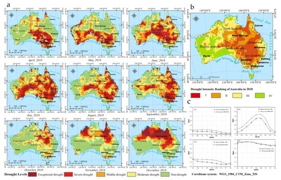
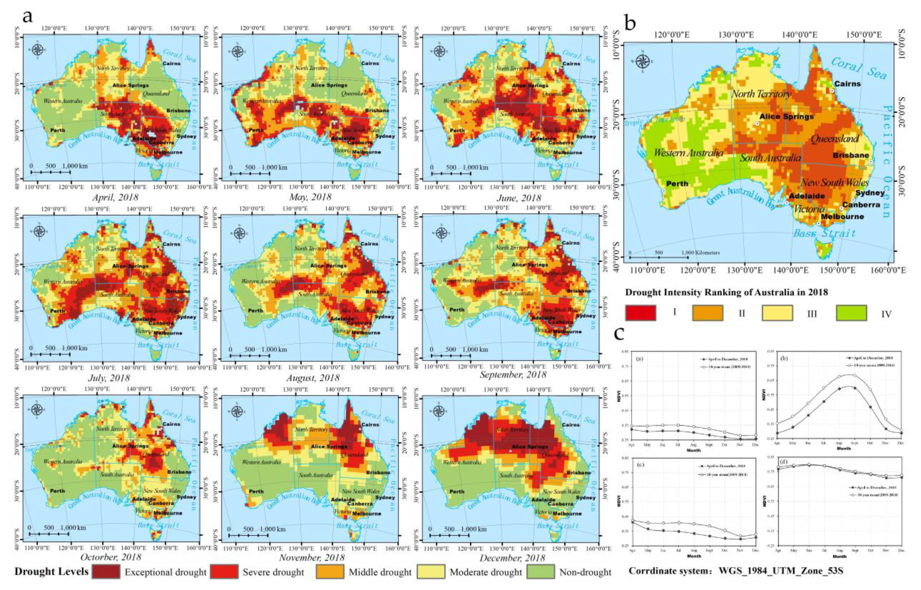
3.1. Monitoring and Evolution of the 2018 Drought Event in Australia

The spatially averaged SPEI across the whole of Australia ranged from −0.77 to −0.08 during January to December of 2018, as shown in Figure 3. In this paper, the given threshold level −0.5 (D0 in Figure 2) was obtained by the drought categorization standard for the drought index of SPEI to discern between a drought and a non-drought. From January to March, the mean SPEI was above the threshold level of −0.5, indicating that no drought occurred. From April to September and from November to December, the mean SPEI was below −0.5, which means that two drought events occurred during these two periods. In particular, the SPEI mean value was below −1 (D1 in Figure 2) in June. However, the mean SPEI was greater than −0.5 and less than 0 (D2 in Figure 2) in October and only lasted for a time interval. Hence, these two drought events in which the SPEI mean value was less than −0.5 during these two periods could be merged into a drought event. Based on the run theory, the Australian drought event of 2018 was identified, and its duration was from April to December.
To explore drought evolution and severity in Australia, the cumulative proportion of the drought area during the past decade (2009–2018) was determined based on the SPEI data with a three-month time scale, as shown in Figure 4. The statistics results from 2009 to 2018 are shown in Figure 4a. The different drought-level percentages for 2018 are reported in Figure 4b. The results showed that the area impacted by exceptional and severe drought in 2018 was extremely large, accounting for 29.31% of the total drought area for the corresponding period, exceeding the average values of the past decade and lasting for a long time. The proportion of drought area (above the level of moderate drought) was up to 88.98% of the total area of Australia, indicating that the 2018 drought was quite severe. During April to December, the proportion of the drought area first increased and then decreased. In July, the drought area reached a high of 68%.
Both the spatiotemporal drought characteristics, examined month by month, and the drought area of each district had notable differences, as presented in Figure 5. The spatiotemporal drought evolution followed a trend in which the drought situation first gradually increased from April to July and subsequently weakened from July to October. However, this trend slowly increased again from November to December. The drought was at its most extreme level in July, as the total drought area, comprising of both exceptional drought and severe drought, accounted for more than 35% of Australia. During the drought duration period, a significant spatiotemporal variation of the distribution of the different drought levels occurred. The drought began in southeastern Australia and widely spread throughout eastern Australia from April to September. In addition, it generally shifted northward from October to December, as seen in Figure 5a. Temporal changes to the drought area proportion (all above the level of moderate drought) of each district were divided into two periods. From April to September, the drought area accounted for more than 90% of Queensland and New South Wales, where the drought was more serious than in other districts. From September to December, the drought area accounted for roughly 50% of Queensland, Victoria and the North Territory, which was the highest level recorded for these districts. During these two periods, the drought area underwent major changes, especially in New South Wales, South Australia, and Western Australia, as shown in Figure 5b. The drought area remained large in the first period but abruptly shrank in the second period, and this trend complements the spatiotemporal distribution shown in Figure 5a.
To study drought severity for the total drought duration, we calculated the mean SPEI, pixel by pixel, to characterize drought intensity from April to December. Four intensity levels were used, and they followed the method of natural breaks classification (NBC) that seeks to minimize the average deviation within the same class mean while maximizing the deviation from the means of the other different classes, and also reduces the variance within classes and maximizes the variance between classes [50,51]. Since the method identifies real classes within the data, it can be advantageous to widely apply in choropleth maps that this method will accurately depict trends delivered in the data [52]. We found that the exceptional drought mainly occurred in southeastern Australia. Drought intensity gradually weakened from southeastern to northwestern Australia, as seen in Figure 5c. It was the strongest in intensity zone I, which was mainly located in the handover zones of three states and includes the southeastern region of North Territory, the northeastern region of South Australia and most parts of Queensland and New South Wales. It accounted for roughly 24% of the total area of Australia. Intensity zone II mainly covered large regions of Queensland, New South Wales and Victoria and the central regions of North Territory and South Australia, accounting for 29% of the total area. Intensity zone III covered the northwestern regions of the North Territory and the northeastern regions of Western Australia, encompassing approximately 28% of the total area. Lastly, intensity zone IV covered the southwestern regions of Western Australia and accounted for 19% of the total area.

3.2. Drought Cause Analysis

SOI fluctuation was notable in 2018 (Figure 6). There was a downward trend from March to September, with a slight upward trend from June to July. Sustained values of the SOI continued to decrease from March and fall below −7 in September, which indicated that an El Niño event occurred in September. Then, the SOI value increased from September and reached more than 7 in December. However, the increasing trend of the SOI value was not continuous but fluctuated; therefore, a La Niña event didn’t occur in December.
The El Niño event in September dramatically increased temperatures and decreased precipitation levels for the coastal zones of Australia, which resulted in drought. Therefore, the percent anomalies of the four meteorological factors were used to investigate the changes to these factors triggered by the El Niño event. To further explore the main meteorological factors caused by the 2018 drought, the annual maximum temperature, total annual precipitation, annual maximum evaporation, and soil moisture in the upper 5 cm of soil were selected to analyze the meteorology anomalies in this study. The anomaly for the annual maximum temperature and anomaly percentages for the other factors in 2018 deviated from the 30-year mean (1989–2018) were calculated by using the anomaly method (Figure 7). We found that the anomaly percentages for the aforementioned factors all had the same distribution characteristic: the most abnormal level for each factor occurred in southeastern Australia. Compared with the past three decades, the anomaly for annual maximum temperature in 2018 was abnormally high, with a maximum of 7.85 °C in southeastern Australia, as shown in Figure 7a. The total annual precipitation for 2018 reached its most severe deficiency level in southeastern Australia, and the highest percent of the negative anomaly was 80.27%, where precipitation in 2018 was only 19.73% of the mean annual precipitation in the reference period (1989–2018), as shown in Figure 7b. The annual maximum evaporation for 2018 negatively deviated 97.03% from the average level of the reference period in southeastern Australia, which was nearly twice that of the past three decades, as shown in Figure 7c. Surface soil moisture (in the upper 5 cm) was lacking in southeastern Australia, with a maximum anomaly percentage of 44.77%, as shown in Figure 7d. Ultimately, the four main meteorological factors all had abnormal values in southeastern Australia during the 2018 drought.
To further investigate the most abnormal meteorological factor that led to the 2018 drought, the CVs and the standardized anomalies Z-score of these factors were calculated, as shown in Table 3. The CVs of the annual maximum temperature, total annual precipitation, annual maximum evaporation, and soil moisture in the upper 5 cm of soil were 0.09, 0.38, 0.31, and 0.12, respectively. Among them, precipitation had the highest CV. The standardized anomalies Z-score of the four meteorological factors were 0.98, −2.39, −0.71, and −1.16, accordingly, in which precipitation also had the highest absolute Z-score value. Both of the CVs and Z-score indicated that total amount of precipitation in 2018 was severely low and abnormal compared with that of the past three decades (1989–2018) more than the other three meteorological factors. Thus, the precipitation deficit was the dominant meteorological element that supported the drought. The spatial distributions of the precipitation deficit, temperature increase, evaporation, and soil-moisture decrease were consistent with the high drought intensity. These results further confirmed that the exceptional drought in southeastern Australia was primarily caused by an abnormal precipitation deficit, coupled with increases in temperature and a decrease in evaporation and soil moisture.

3.3. Drought Impacts on Vegetation Growth

3.3.1. Drought Impacts on NDVI

Since NDVI is a vegetation index widely used to reflect vegetation growth, a comparison between mean NDVI values for 2018 and for the past decade can be used to illustrate the drought impacts on vegetation growth. The mean NDVI values for all land-cover types (cropland, grassland, and forest) were presented in Figure 8. The mean NDVI values for 2018 were significantly lower than the average (Figure 8a–c), although the difference was not as extreme for the forest value (Figure 8d). Obviously, the curve of cropland was very different from those of the other vegetation types, as the result of which the main types of crops grown in Australia were wheat and barley, which were generally sown from the end of April to the beginning of July, and harvest in October to January of the next year, the duration period of the 2018 drought was exactly the key growth period of wheat and barley. Therefore, the curve of cropland showed a trend of first increasing from April to September and then decreasing, which was barely the same with the other three [53]. Both of those indicated that the exceptional drought greatly affected vegetation growth in Australia, especially for cropland and grassland.
To analyze drought impacts on different land-cover types, the mean NDVI values for April to December of 2018 and from the same period for the past decade were calculated. For this purpose, the standardized anomalies Z-score of NDVI for all land-cover types (cropland, grassland, and forest) was also calculated. When we compared the Z-score of NDVI values for 2018 and the past decade, the difference of drought impacts on vegetation growth for different land-cover types became clear (Figure 9). In September, the worst negative Z-score, aside from the whole drought duration, occurred in the NDVI value for all land-cover types, grassland, and forest land, as they had approximately −0.73, −0.76, and −0.44 Z-scores that deviated from the 10-year mean value, respectively. The NDVI for cropland demonstrated a negative Z-score peak of −1.03 in October. The Z-score for cropland was significantly lower than that of the other land-cover types, followed by grassland and forest, accordingly. These results showed that the exceptional drought had significant impacts on vegetation growth derived by NDVI, and cropland and grassland were the most affected. Relatively speaking, forest was not significantly affected.

3.3.2. Drought Impacts on SIF

When compared with that of the value for the past decade (2009–2018), the curve of the mean SIF value for 2018 revealed a significant SIF fluctuation caused by the exceptional drought, especially in October; this comparison was shown in Figure 10. The mean SIF values for all the land-cover types, grassland, and forest all declined slightly and then increased significantly, subsequently following a slight downward trend, as represented in Figure 10a,c,d, respectively. The SIF curve for cropland gradually rose and then decreased, as shown in Figure 10b. Similarly, the same characteristic of SIF changes for cropland was also found in which the SIF curve of cropland was very different from those of the other vegetation types, and the same reason with the curve for cropland reflected by NDVI was supplied. The mean SIF value for 2018 was significantly lower than the average of the past decade among all the land-cover types, cropland, grassland, and forest, which demonstrated that the exceptional drought greatly affected SIF.
Overall, the Z-score curves of SIF for all land-cover types, cropland, grassland, and forest followed the same trend, epitomized by the curve for cropland (Figure 11). The SIF Z-score for cropland demonstrated two negative peaks, −1.12 in October, followed by August (−1.08). The worst SIF Z-score for all land-cover types occurred in October (approximately −0.53); grassland in August (approximately −0.67), and forest land in October (approximately −0.75). The occurrence time of the worst Z-score for forest land was wholly consistent with cropland, during which they were the most affected by the exceptional drought. Our results suggested that SIF was greatly impacted by the exceptional drought. We found that the mean precipitation in October (approximately 15.88 mm) was at an extremely low level throughout the drought duration, second only to September (approximately 8.71 mm) during April to December in 2018, during which cropland and forest land were therefore the most affected in October, grassland was the most affected in September, to a certain extent; this conclusion is consistent with the NDVI drought response.

3.3.3. Diverse Droughts Responses by NDVI and SIF

To analyze the sensitivity difference of NDVI and SIF in detecting drought impacts, the drought responses of NDVI and SIF to SPEI were compared. The correlation curves for NDVI Z-score, SIF Z-score, and SPEI for the different land-cover types (cropland, grassland, and forest) were compared using a scatter plot method. We found that the linear correlation between SIF and SPEI was greater than that between NDVI and SPEI (Figure 12). For each land-cover type, r was 0.7174 in a linear relationship between the SIF for cropland and SPEI (p < 0.01; Figure 12d). The correlation r was only 0.3366 and 0.4946 for both grassland and forest and SPEI (p < 0.05), shown in Figure 12e,f, respectively. However, the correlation between the NDVI for grassland, the NDVI for forest, and SPEI did not pass the significance test (Figure 12b,c). Only the NDVI for cropland passed, and the correlation coefficient r was 0.5503 (p < 0.05; Figure 12a). These results revealed a clear correlation between SIF and SPEI, of which the correlation between SIF and SPEI was higher than NDVI, which further demonstrated that SIF responded to drought better than NDVI. In summary, SIF was superior to NDVI in detecting drought impacts.

4. Discussion

4.1. Drought Characteristics and Cause

Our study found that the intensity of the exceptional drought gradually decreased from northwestern to southeastern Australia and reached its highest level in southeastern Australia. This effect was notable in the junction zone of Queensland, New South Wales, and Southern Australia. The drought mainly resulted from a lack of precipitation coupled with abnormal temperature, evaporation, and soil moisture conditions, as seen in Figure 7 and Table 3. Previous studies reported that several drought hotspots were frequently reactivated during recent decades, and southern Australia is one of the most severe drought hotspots, with a notable increase in drought frequency and duration over time. Australia is frequently attacked by droughts resulting from abnormal climate events, such as EI Niño events, which leads to progressive temperature increases that are not balanced by precipitation increases [54,55,56]. Drought is usually caused by an extreme lack of precipitation and a severe increase in temperature. Since an abnormal temperature directly leads to a dramatic increase in evapotranspiration, soil moisture becomes reduced by a large margin. Notably, precipitation varies more than other meteorological factors [33,57], which our results confirmed to a certain extent.

4.2. Drought Impacts

Previous studies showed that both NDVI and SIF can reflect vegetation growth and take advantage of remote sensing methods. NDVI characterizes the vegetation greenness, which can track changes in vegetation condition caused by drought to some extent [58]. In contrast, SIF reflects vegetation photosynthesis [23]. Therefore, NDVI and SIF respond differently to drought. Generally, vegetation greenness indices (such as NDVI and EVI) have significant lags in response to drought [24]. For instance, the lag period for NDVI ranges from 10 days to two months [59]. Our study found that the most serious drought in southeastern Australia occurred in July, while NDVI and SIF were greatly affected during September to October. This discrepancy was consistent with previous research.
We also found that the exceptional drought had an important impact on NDVI and SIF (Figure 8 and Figure 10). Of the different land-cover types, cropland was more affected by the exceptional drought than grassland and forest, which supports the conclusion that cropland is more likely to be affected by drought [60]. After analyzing the correlations between NDVI, SIF, and SPEI, we concluded that SIF was superior to NDVI. This result supports the previous conclusion that SIF is a more effective drought response indicator than NDVI [50,61]. Nonetheless, our correlations for both NDVI, SIF, and SPEI were less than 0.6, which was mainly due to the 0.5° × 0.5° spatial resolution for SPEI and SIF. When SPEI and SIF were masked and extracted using the land-cover data at 1 × 1 km spatial resolution, one SIF pixel at 0.5° × 0.5° units may contain multiple land-cover types (cropland, grassland, and forest land); however, SIF values for different land-cover types was barely the same, it would be possible for the fixed pixels in our SPEI and SIF extractions by different land-cover types to cause problems [62]. In particular, the extraction process was bound to result in weak correlations between NDVI, SIF, and SPEI for different land-cover types.
Irrigation and planting structure adjustments are two of the most effective measures to prevent drought and lessen drought impacts on agricultural plant zones [63]. Notably, irrigation measures can effectively improve the near-surface climate conditions on a global scale [64]. In this study, we also analyzed the effect of drought prevention and relief measures by using NDVI to compare the different drought responses of irrigated croplands and rainfed croplands (Figure 13). Two typical sampling areas mainly distributed in the southeastern part of Australia that experienced the most severe drought intensity levels, ranging from the east to west side of the Great Dividing Range, respectively, were selected to analyze these different responses, as shown in Figure 13a. We found that the NDVI of the irrigated croplands was larger than that of the rainfed croplands from April to December of 2018, and the response differences were more significant on the west side of the Great Dividing Range than the east, as shown in Figure 13b,c, which could reflect the effect of drought prevention and relief measures to some extent. The quantitative evaluation of the socioeconomic impacts of drought and exploration of drought control and drought resistance measures, such as irrigation measures, is a possible area of further study.

4.3. Response Revelation of the Exceptional Drought to SDGs

Drought loss can be effectively reduced through the reasonable adjustment of planting structures and the implementation of compatible irrigation steps when the drought risk is at its highest [49]. Since it is the driest inhabited continent and has a high drought risk, Australia faces many drought-related challenges, and feasible management strategies to prevent drought loss have been developed specifically for Australia, especially for its agricultural sector [60]. The Australian Department of Agriculture and Water Resources timely adjusted the agricultural planting structure in 2019, and the total area of summer crops was reduced by about 1 million hectares, which is a 23% decrease from the same period in 2018–2019. The cotton planting area also fell by 44%. In addition, the Australian government plans to set up a future drought fund worth $5 billion and to allocate $100 million annually to continuously improve drought resistance measures and reduce drought damage. To a certain extent, these strategies are in line with the Agricultural Productivity and Sustainable Agriculture Proportion’ measure in the Sustainable Development Goals (SDGs) published by the United Nations. These goals have the following specification: “By 2030, ensure the establishment of sustainable food production systems and the implementation of resilience-based farming practices. Monitoring the drought prevention measures undertaken by the Australian government will help guide long-term drought responses for this region”.
In this study, we examined the drought mechanism of the exceptional drought event that occurred across southeastern Australia from April to December in 2018. In addition, we also depicted the drought evolution process and explored drought causes and impacts on NDVI and SIF. This study responds to an urgent need for drought research and provides guidance on how to formulate timely and effective drought response measures. Therefore, this study would contribute to the realistic demand for the sustainable socioeconomic development of Australia.

5. Conclusions

In 2018, an exceptional drought event occurred in southeastern Australia. In particular, regions in Queensland, New South Wales, and Victoria were affected, and drought intensity conformed with the spatial distribution characteristics of insufficient precipitation, increased temperature, increased evapotranspiration, and decreased soil moisture. These characteristics were influenced by an EI Niño event that occurred in September 2018. Overall, the Australian drought event was caused by extreme lack of precipitation. Notably, the drought had long-term impacts on the vegetation in these regions, as measured using the Normalized Difference Vegetation Index (NDVI) and sun-induced chlorophyll fluorescence (SIF). When accounting for different land-cover types, NDVI and SIF levels during the drought period, from April to December 2018, were significantly less than the average levels of the previous decade (2009–2018). The exceptional drought greatly affected cropland. Furthermore, we also found that SIF is superior to NDVI in detecting drought impacts.

Author Contributions

Author Contributions: Conceptualization, F.T. and J.W.; methodology, F.T. and J.Y.; resources, S.L.; software, L.L.; validation, F.T. and L.L.; formal analysis, F.T. and L.L.; investigation, W.Z. and Q.S.; writing—review and editing, F.T. and L.L. All authors have read and agreed to the published version of the manuscript.

Funding

This research was funded by National Key Research and Development Project of China, grant number 2017YFB0504102; Natural Science Foundation of China, grant number 41671424.

Acknowledgments

We would like to thank sincerely the editor and anonymous reviewers for their constructive suggestions and improvements to our work.

Conflicts of Interest

The authors declare no conflict of interest.

References

  1. Ghil, M.; Vautard, R. Interdecadal oscillations and the warming trend in global temperature time series. Nature 1991, 350, 324–327. [Google Scholar] [CrossRef]
  2. Solomon, S.; Plattner, G.K.; Knutti, R.; Friedlingstein, P. Irreversible climate change due to carbon dioxide emissions. Proc. Natl. Acad. Sci. USA 2009, 106, 1704–1709. [Google Scholar] [CrossRef] [Green Version]
  3. IPCC. Special Report on Global Warming of 1.5 °C; Cambridge University Press: Cambridge, UK, 2018. [Google Scholar]
  4. Prospero, J.M.; Nees, R.T. Impact of the North African drought and EI-Niño on mineral dust in the Barbados trade winds. Nature 1986, 320, 735–738. [Google Scholar] [CrossRef]
  5. Cai, W.J.; Santoso, A.; Wang, G.J.; Yeh, S.W.; An, S.I.; Cobb, K.M.; Collins, M.; Guilyardi, E.; Jin, F.F.; Kug, J.S.; et al. ENSO and greenhouse warming. Nat. Clim. Chang. 2015, 5, 849–859. [Google Scholar] [CrossRef]
  6. Madadgar, S.; Moradkhani, H. Spatio-temporal drought forecasting within Bayesian networks. J. Hydrol. 2014, 512, 134–146. [Google Scholar] [CrossRef]
  7. Dehghani, M.; Saghafian, B.; Saleh, F.N.; Farokhnia, A.; Noorie, R. Uncertainty analysis of streamflow drought forecast using artificial neural networks and Monte-Carlo simulation. Int. J. Climatol. 2014, 34, 1169–1180. [Google Scholar] [CrossRef]
  8. Held, I.M.; Soden, B.J. Robust responses of the hydrological cycle to global warming. J. Clim. 2006, 19, 5686–5699. [Google Scholar] [CrossRef]
  9. Seager, R.; Vecchi, G.A. Greenhouse warming and the 21st century hydroclimate of southwestern North America. Proc. Natl. Acad. Sci. USA 2010, 107, 21277–21282. [Google Scholar] [CrossRef] [PubMed] [Green Version]
  10. Feng, H.; Zhang, M. Global land moisture trends: Drier in dry and wetter in wet over land. Sci. Rep. 2015, 5, 18018. [Google Scholar] [CrossRef] [PubMed]
  11. Zuo, D.P.; Cai, S.Y.; Xu, Z.X.; Peng, D.Z.; Kan, G.Y.; Sun, W.C.; Pang, B.; Yang, H. Assessment of meteorological and agricultural droughts using in-situ observations and remote sensing data. Agric. Water Manag. 2019, 222, 125–138. [Google Scholar] [CrossRef]
  12. Mishra, A.K.; Singh, V.P. A review of drought concepts. J. Hydrol. 2010, 391, 202–216. [Google Scholar] [CrossRef]
  13. Feng, P.Y.; Wang, B.; Liu, D.L.; Yu, Q. Machine learning-based integration of remotely-sensed drought factors can improve the estimation of agricultural drought in South-Eastern Australia. Agric. Syst. 2019, 173, 303–316. [Google Scholar] [CrossRef]
  14. Mpelasoka, F.; Awange, J.L.; Goncalves, R.M. Accounting for dynamics of mean precipitation in drought projections: A case study of Brazil for the 2050 and 2070 periods. Sci. Total Environ. 2018, 622–623, 1519–1531. [Google Scholar] [CrossRef] [PubMed]
  15. Lu, J.Y.; Carbone, G.J.; Grego, J.M. Uncertainty and hotspots in 21st century projections of agricultural drought from CMIP5 models. Sci. Rep. 2019, 9, 4922. [Google Scholar] [CrossRef]
  16. Haile, G.G.; Tang, Q.H.; Sun, S.; Huang, Z.W.; Zhang, X.J.; Liu, X.C. Droughts in East Africa: Causes, impacts and resilience. Earth Sci. Rev. 2019, 193, 146–161. [Google Scholar] [CrossRef]
  17. Shiru, M.S.; Shahid, S.; Chung, E.S.; Alias, N. Changing characteristics of meteorological droughts in Nigeria during 1901–2010. Atmos. Res. 2019, 223, 60–73. [Google Scholar] [CrossRef]
  18. Howden, M.; Schroeter, S.; Crimp, S.; Hanigan, I. The changing roles of science in managing Australian droughts: An agricultural perspective. Weather Clim. Extrem. 2014, 3, 80–89. [Google Scholar] [CrossRef] [Green Version]
  19. Tweed, S.; Leblanc, M.; Cartwright, I. Groundwater–surface water interaction and the impact of a multi-year drought on lakes conditions in South-East Australia. J. Hydrol. 2009, 379, 41–53. [Google Scholar] [CrossRef]
  20. Ciais, P.; Reichstein, M.; Viovy, N.; Granier, A.; Ogee, J.; Allard, V.; Aubinet, M.; Buchmann, N.; Bernhofer, C.; Carrara, A.; et al. Europe-wide reduction in primary productivity caused by the heat and drought in 2003. Nature 2005, 437, 529–533. [Google Scholar] [CrossRef]
  21. Van der Velde, M.; Tubiello, F.N.; Vrieling, A.; Bouraoui, F. Impacts of extreme weather on wheat and maize in France: Evaluating regional crop simulations against observed data. Clim. Chang. 2012, 113, 751–765. [Google Scholar] [CrossRef] [Green Version]
  22. Schwalm, C.R.; Anderegg, W.R.L.; Michalak, A.M.; Fisher, J.B.; Biondi, F.; Koch, G.; Litvak, M.; Ogle, K.; Shaw, J.D.; Wolf, A.; et al. Global patterns of drought recovery. Nature 2017, 548, 202–205. [Google Scholar] [CrossRef] [PubMed]
  23. Li, X.Y.; Li, Y.; Chen, A.P.; Gao, M.D.; Slette, I.J.; Piao, S.L. The impact of the 2009/2010 drought on vegetation growth and terrestrial carbon balance in Southwest China. Agric. For. Meteorol. 2019, 269–270, 239–248. [Google Scholar] [CrossRef]
  24. Ji, L.; Peters, A.J. Assessing vegetation response to drought in the northern Great Plains using vegetation and drought indices. Remote Sens. Environ. 2003, 87, 85–98. [Google Scholar] [CrossRef]
  25. Liu, L.Z.; Yang, X.; Zhou, H.K.; Liu, S.S.; Zhou, L.; Li, X.H.; Yang, J.H.; Han, X.Y.; Wu, J.J. Evaluating the utility of solar-induced chlorophyll fluorescence for drought monitoring by comparison with NDVI derived from wheat canopy. Sci. Total Environ. 2018, 625, 1208–1217. [Google Scholar] [CrossRef] [PubMed]
  26. Song, L.; Guanter, L.; Guan, K.Y.; You, L.Z.; Huete, A.; Ju, W.M.; Zhang, Y.G. Satellite sun-induced chlorophyll fluorescence detects early response of winter wheat to heat stress in the Indian Indo-Gangetic Plains. Glob. Chang. Biol. 2018, 24, 4023–4037. [Google Scholar] [CrossRef] [PubMed] [Green Version]
  27. Vicente-Serrano, S.M.; Beguería, S.; López-Moreno, J.I. A Multi-scalar drought index sensitive to global warming: The standardized precipitation evapotranspiration index–SPEI. J. Clim. 2010, 23, 1696–1718. [Google Scholar] [CrossRef] [Green Version]
  28. Palmer, W.C. Keeping track of crop moisture conditions, nationwide: The new crop moisture index. Weatherwise 1968, 21, 156–161. [Google Scholar] [CrossRef]
  29. McKee, T.B.; Doesken, N.J.; Kleist, J. The Relationship of Drought Frequency and Duration to Time Scales. Presented at the 8th Conference on Applied Climatology, Boston, MA, USA, 17–22 January 1993; American Meteorological Society: Anaheim, CA, USA, 1993. [Google Scholar]
  30. Liu, W.T.; Kogan, F.N. Monitoring regional drought using the vegetation condition index. Int. J. Remote Sens. 1996, 17, 2761–2782. [Google Scholar] [CrossRef]
  31. Sandholi, I.; Rasmussen, K.; Ersen, J. A simple interpretation of the surface temperature vegetation index space for assessment of surface moisture status. Remote Sens. Environ. 2002, 79, 213–214. [Google Scholar] [CrossRef]
  32. Lewis, S.L.; Brando, P.M.; Phillips, O.L.; Van der Heijden, G.M.F.; Nepstad, D. The 2010 Amazon Drought. Science 2011, 331, 554. [Google Scholar] [CrossRef]
  33. Ci, H.; Zhang, Q.; Xiao, M.Z. Evaluation and comparability of four meteorological drought indices during drought monitoring in Xinjiang. Acta Sci. Nat. Univ. Sunyatseni 2016, 55, 124–133. [Google Scholar]
  34. Pritchard, H.D. Asia’s shrinking glaciers protect large populations from drought stress. Nature 2019, 569, 649–654. [Google Scholar] [CrossRef] [PubMed]
  35. Wang, W.; Zhu, Y.; Xu, R.G.; Liu, J.T. Drought severity change in China during 1961–2012 indicated by SPI and SPEI. Nat. Hazards 2015, 75, 2437–2451. [Google Scholar] [CrossRef]
  36. Kamali, B.; Abbaspour, K.C.; Wehrli, B.; Yang, H. Drought vulnerability assessment of maize in Sub-Saharan Africa: Insights from physical and social perspectives. Glob. Planet. Chang. 2018, 162, 266–274. [Google Scholar] [CrossRef] [Green Version]
  37. Leng, G.Y.; Hall, J. Crop yield sensitivity of global major agricultural countries to droughts and the projected changes in the future. Sci. Total Environ. 2019, 654, 811–821. [Google Scholar] [CrossRef] [PubMed]
  38. Dai, A.G. Drought under global warming: A review. WIREs Clim. Chang. 2011, 2, 45–65. [Google Scholar] [CrossRef] [Green Version]
  39. Forootan, E.; Khaki, M.; Schumacher, M.; Wulfmeyer, V.; Mehrnegar, N.; Van Dijk, A.I.J.M.; Brocca, L.; Farzaneh, S.; Akinluyi, F.; Ramillien, G.; et al. Understanding the global hydrological droughts of 2003–2016 and their relationships with teleconnections. Sci. Total Environ. 2019, 650, 2587–2604. [Google Scholar] [CrossRef] [Green Version]
  40. Wilhite, D.A.; Glantz, M.H. Understanding: The drought phenomenon: The role of definitions. Water Int. 1985, 10, 111–120. [Google Scholar] [CrossRef] [Green Version]
  41. Spinoni, J.; Barbosa, P.; Jager, A.D.; McCormick, N.; Naumann, G.; Vogt, J.V.; Magni, D.; Masante, D.; Mazzeschi, M. A new global database of meteorological drought events from 1951 to 2016. J. Hydrol. Reg. Stud. 2019, 22, 100593. [Google Scholar] [CrossRef]
  42. Kirono, D.G.C.; Kent, D.M.; Hennessy, K.J.; Mpelasoka, F. Characteristics of Australian droughts under enhanced greenhouse conditions: Results from 14 global climate models. J. Arid Environ. 2011, 75, 566–575. [Google Scholar] [CrossRef]
  43. Kim, T.W.; Valdes, J.B.; Nijssen, B.; Roncayolo, D. Quantification of linkages between large-scale climatic patterns and precipitation in the Colorado River Basin. J. Hydrol. 2006, 321, 173–186. [Google Scholar] [CrossRef]
  44. Wang, X.M.; Zhang, K.F.; Wu, S.Q.; Li, Z.S.; Cheng, Y.Y.; Li, L.; Yuan, H. The correlation between GNSS-derived precipitable water vapor and sea surface temperature and its responses to El Niño–Southern Oscillation. Remote Sens. Environ. 2018, 216, 1–12. [Google Scholar] [CrossRef]
  45. Zhao, H.Y.; Gao, G.; An, W.; Zhou, X.K.; Li, H.T.; Hou, M.T. Timescale differences between SC-PDSI and SPEI for drought monitoring in China. Phys. Chem. Earth 2017, 102, 48–58. [Google Scholar] [CrossRef]
  46. Soh, Y.W.; Koo, C.H.; Huang, Y.F.; Fung, K.F. Application of artificial intelligence models for the prediction of standardized precipitation evapotranspiration index (SPEI) at Langat River Basin, Malaysia. Comput. Electron. Agric. 2018, 144, 164–173. [Google Scholar] [CrossRef]
  47. Van Hateren, T.C.; Sutanto, S.J.; Van Lanen, H.A.J. Evaluating skill and robustness of seasonal meteorological and hydrological drought forecasts at the catchment scale—Case Catalonia (Spain). Environ. Int. 2019, 133, 105206. [Google Scholar] [CrossRef]
  48. Guo, H.; Bao, A.M.; Liu, T.; Jiapaer, G.; Ndayisaba, F.; Jiang, L.L.; Kurban, A.; Maeyer, P.D. Spatial and temporal characteristics of droughts in Central Asia during 1966–2015. Sci. Total Environ. 2018, 624, 1523–1538. [Google Scholar] [CrossRef]
  49. Mishra, A.K.; Singh, V.P.; Desai, V.R. Drought characterization: A probabilistic approach. Stoch. Environ. Res. Risk Assess. 2009, 23, 41–55. [Google Scholar] [CrossRef]
  50. Jenks, G.F. The data model concept in statistical mapping. Int. Yearb. Cartogr. 1967, 7, 186–190. [Google Scholar]
  51. Jenks, G.F.; Fred, C.C. Error on Chloroplethic Maps: Definition, Measurement, Reduction. Ann. Assoc. Am. Geogr. 1971, 61, 217–244. [Google Scholar] [CrossRef]
  52. McMaster, R. In Memoriam: George, F. Jenks (1916–1996). Cartogr. Geogr. Inf. Sci. 1997, 24, 56–59. [Google Scholar] [CrossRef]
  53. Shaaban, A.S.A.; Wahbi, A.; Sinclair, T.R. Sowing date and mulch to improve water use and yield of wheat and barley in the Middle East environment. Agric. Syst. 2018, 165, 26–32. [Google Scholar] [CrossRef]
  54. Kiem, A.S.; Franks, S.W. Multi-decadal variability of drought risk, eastern Australia. Hydrol. Process. 2004, 18, 2039–2050. [Google Scholar] [CrossRef]
  55. Spinoni, J.; Naumann, G.; Carrao, H.; Barbosa, P.; Vogt, J. World drought frequency, duration, and severity for 1951–2010. Int. J. Climatol. 2014, 34, 2792–2804. [Google Scholar] [CrossRef] [Green Version]
  56. Nandintsetseg, B.; Shinoda, M.; Du, C.L.; Munkhjargal, E. Cold-season disasters on the Eurasian steppes: Climate-driven or man-made. Sci. Rep. 2018, 8, 14769. [Google Scholar] [CrossRef] [PubMed]
  57. Nanzad, L.; Zhang, J.H.; Tuvdendorj, B.; Nabil, M.; Zhang, S.; Bai, Y. NDVI anomaly for drought monitoring and its correlation with climate factors over Mongolia from 2000 to 2016. J. Arid Environ. 2019, 164, 69–77. [Google Scholar] [CrossRef]
  58. Di, L.P.; Rundquist, D.C.; Han, L.H. Modeling relationships between NDVI and precipitation during vegetative growth cycles. Int. J. Remote Sens. 1994, 15, 2121–2136. [Google Scholar] [CrossRef]
  59. Doughty, R.; Xiao, X.M.; Wu, X.C.; Zhang, Y.; Bajgain, B.; Zhou, Y.T.; Qin, Y.W.; Zou, Z.H.; McCarthy, H.; Friedman, J.; et al. Responses of gross primary production of grasslands and croplands under drought, pluvial, and irrigation conditions during 2010–2016, Oklahoma, USA. Agric. Water Manag. 2018, 204, 47–59. [Google Scholar] [CrossRef]
  60. Liu, L.Z.; Yang, X.; Zhou, H.K.; Liu, S.S.; Zhou, L.; Li, X.H.; Yang, J.H.; Wu, J.J. Relationship of root zone soil moisture with solar-induced chlorophyll fluorescence and vegetation indices in winter wheat: A comparative study based on continuous ground-measurements. Ecol. Indic. 2018, 90, 9–17. [Google Scholar] [CrossRef]
  61. Kiem, A.S.; Austin, E.K. Drought and the future of rural communities: Opportunities and challenges for climate change adaptation in regional Victoria, Australia. Glob. Environ. Chang. 2013, 23, 1307–1316. [Google Scholar] [CrossRef] [Green Version]
  62. Jones, H.G.; Sirault, X.R.R. Scaling of Thermal Images at Different Spatial Resolution: The Mixed Pixel Problem. Agronomy 2014, 4, 380–396. [Google Scholar] [CrossRef] [Green Version]
  63. Wilhite, D.A.; Sivakumar, M.V.K.; Pulwarty, R. Managing drought risk in a changing climate: The role of national drought policy. Weather Clim. Extrem. 2014, 3, 4–13. [Google Scholar] [CrossRef] [Green Version]
  64. Puma, M.J.; Cook, B.I. Effects of irrigation on global climate during the 20th century. J. Geophys. Res. 2010, 115. [Google Scholar] [CrossRef]
Figure 1. Australia’s climatic zones and land-cover types.
Remotesensing 12 00054 g001
Figure 2. Drought events identification based on run theory.
Remotesensing 12 00054 g002
Figure 3. Determination of Australian drought duration in 2018 based on run theory.
Remotesensing 12 00054 g003
Figure 4. Changes in the drought area of Australia using times-series analysis. In (a), the accumulated area percentages for the different drought levels over the past decade were shown. The legend “Moderate up to Exceptional droughts” in (a) represents the area percentage that accounts for the total drought area including grid cells affected by moderate up to exceptional droughts. Similarly, “Middle up to Exceptional droughts” represents the area percentage that accounts for the total drought area affected by middle up to exceptional droughts, “Severe up to Exceptional droughts” represents the area percentage that accounts for the total drought area affected by severe up to exceptional droughts, and “Exceptional drought” represents the area percentage that accounts for the total drought area affected by exceptional drought. In (b), the area percentages for the different drought levels from April to December of 2018 are shown.
Remotesensing 12 00054 g004
Figure 5. The spatiotemporal drought evolution for the entire drought duration period. In (a), the spatiotemporal distribution during the drought duration period was showed month by month. In (b), the drought area (above the level of moderate drought) relative to the total area of each district is shown. In (c), the drought intensity for Australia in 2018 was presented.
Remotesensing 12 00054 g005
Figure 6. Southern oscillation index (SOI) values from January to December 2018.
Remotesensing 12 00054 g006
Figure 7. Anomaly for annual maximum temperature (a), and anomaly percentages for the other meteorological factors in 2018 were presented, compared with the past three decades (1989–2018): (b) Total annual precipitation, (c) annual maximum evaporation, and (d) soil moisture in the upper 5 cm of soil.
Remotesensing 12 00054 g007
Figure 8. Comparison of mean NDVI values for (a) all land-cover types, (b) cropland, (c) grassland and (d) forest from April to December 2018 and for the same period over the past decade in Australia (the black line with a solid circle represents the mean value from April to December 2018, and the black line with a hollow circle represents the 10-year mean value from 2009 to 2018).
Remotesensing 12 00054 g008
Figure 9. The standardized anomalies Z-score for NDVI from April to December 2018 and for the same period over the past decade in Australia.
Remotesensing 12 00054 g009
Figure 10. A comparison of the mean SIF values for (a) all land-cover types, (b) cropland, (c) grassland, and (d) forest from April to December 2018 and for the same period over the past decade in Australia (the black line with a solid circle represents the mean value from April to December 2018, and the black line with a hollow circle represents the 10-year mean value from 2009 to 2018).
Remotesensing 12 00054 g010
Figure 11. The standardized anomalies Z-score for SIF from April to December 2018 and for the same period over the past decade in Australia.
Remotesensing 12 00054 g011
Figure 12. The correlation curve between SPEI and the Z-score of NDVI for (a) cropland, (b) grassland, and (c) forest land, SIF for (d) cropland, (e) grassland, and (f) forest land (the black line represents the linear fit).
Remotesensing 12 00054 g012
Figure 13. The response differences of NDVI between irrigated croplands and rainfed croplands to drought. In (a), the location of the two selected sampling areas was shown, and in (b,c), the NDVI comparison between irrigated croplands and rainfed croplands in the east side and west side of the Great Dividing Range were presented, respectively (the black line with a solid circle represents the mean value for rainfed croplands from April to December in 2018, and the black line with a hollow circle represents the mean value for irrigated cropland from April to December in 2018).
Remotesensing 12 00054 g013
Table 1. The ranking division standard of the Standardized Precipitation Evapotranspiration Index (SPEI).
Value RangeSPEI ≤ −2−2 < SPEI ≤ −1.5−1.5 < SPEI ≤ −1−1 < SPEI ≤ −0.5SPEI > −0.5
LevelsExceptional droughtSevere droughtMiddle droughtModerate droughtNon-drought
Table 2. Summary of the data sets exploited in the analysis. AVDC: Aura Validation Data Center, ECMWF: European Centre for Medium-Range Weather Forecasts, NASA: National Aeronautics and Space Administration, NDVI: Normalized Difference Vegetation Index, SIF: sun-induced chlorophyll fluorescence, SOI: Southern Oscillation Index, SPEI: Standardized Precipitation Evapotranspiration Index.
Data TypeData NameResolutionTime RangeData Source
SpatialTemporal
SPEI030.5° × 0.5°Monthly2009–2018SPEI Global drought monitor
Land coverMCD12Q1500 × 500 mYearly2018NASA LPDAAC
NDVIMOD13A31 × 1 kmMonthly2009–2018
TemperatureERA5 monthly averaged data on single levels0.25° × 0.25°Monthly1989–2018ECMWF
Precipitation
Evaporation
SIFGOME-020.5° × 0.5°Monthly2009–2018AVDC
Soil moistureESA soil moisture gridded dataset0.25° × 0.25°Monthly1989–2018ECMWF
SOISouthern Oscillation IndexMonthly2018Bureau of Meteorology Australia
Table 3. Coefficient of variations (CVs) and the standardized anomalies Z-score of the four main meteorological factors: annual maximum temperature, total annual precipitation, maximum annual evaporation, and soil moisture in the upper 5 cm of soil.
Meteorological FactorsAnnual Maximum TemperatureTotal Annual PrecipitationMaximum Annual EvaporationSoil Moisture in the Upper 5 cm of Soil
CV0.090.380.310.12
Z-score0.98−2.39−0.71−1.16

