Article

Tree Species (Genera) Identification with GF-1 Time-Series in A Forested Landscape, Northeast China

1
School of Resources and Environmental Engineering, Hefei University of Technology, Hefei 230009, China
2
International Institute for Earth System Science, Nanjing University, Nanjing 210023, China
3
Institute for Spatial Information Intelligence Analysis and Application, Hefei University of Technology, Hefei 230009, China
4
Department of Life Science, Tunghai University, Taichung 40704, Taiwan
5
Center for Ecology and Environment, Tunghai University, Taichung 40704, Taiwan
*
Author to whom correspondence should be addressed.
Remote Sens. 2020, 12(10), 1554; https://doi.org/10.3390/rs12101554
Submission received: 23 April 2020 / Revised: 11 May 2020 / Accepted: 12 May 2020 / Published: 13 May 2020
(This article belongs to the Section Forest Remote Sensing)

Abstract

:
Forests are the most important component of terrestrial ecosystem; the accurate mapping of tree species is helpful for the management of forestry resources. Moderate- and high-resolution multispectral images have been commonly utilized to identify regional tree species in forest ecosystem, but the accuracy of recognition is still unsatisfactory. To enhance the forest mapping accuracy, this study integrated the land surface phenological metrics and text features of forest canopy on tree species identification based on Gaofen-1 (GF-1) wide field of view (WFV) and time-series images (36 10-day NDVI data), conducted at a forested landscape in Harqin Banner, Northeast China in 2017. The dominant tree species include Pinus tabulaeformis, Larix gmelinii, Populus davidiana, Betula platyphylla, and Quercus mongolica in the study region. The result of forest mapping derived from a 10-day dataset was also compared with the outcome based upon a commonly utilized 30-day dataset in tree species identification. The results indicate that tree species identification accuracy is significantly (p < 0.05) improved with higher temporal resolution (10-day, 79.4%) of images than commonly used monthly data (30-day, 76.14%), and the accuracy can be further increased to 85.13% with a combination of the information derived from principal component analysis (PCA) transformation, phenological metrics (standing for the information of growing season) and texture features. The integration of higher dimensional NDVI data, vegetation growth dynamics and feature of canopy simultaneously will be beneficial to map tree species at the landscape scale.

Graphical Abstract

1. Introduction

Forest is one of the most important components of the global terrestrial ecosystem, which covers about one third of the earth’s land surface [1]. An accurate understanding the patterns of tree species is required to reasonably utilize and manage regional forest resources [2,3]. Remotely sensed data are considered an effective method to identify tree species or forest types at broader scale [4,5], and the higher resolution of satellite images can avoid the spectral distortion of vegetation caused by mixed pixels and is helpful to identify forest patterns [6,7,8]. Compared to airborne hyperspectral and light detection and ranging (LiDAR) data, the multispectral satellite images with higher spatiotemporal scale, larger spatial coverage and lower expense have shown great potential for the identification of tree species at regional scale [8,9].
Studies showed that the in situ observations of the seasonal growth of vegetation, including budburst, leaf development, flowering, leaf coloring, senescence and dormancy, indicated that these phenological phases varied from species to species, and differed among regions [10,11,12]. The field works were invaluable, but their representative was sometimes limited by a smaller spatial extent, and they were scarce in remote regions. In contrast, the advancement in remotely sensed data on spatiotemporal scale over time had been proved to be not only effective for identifying tree species, but also be powerful for delineating the seasonal dynamics of canopy dominant species [13,14]. For example, the Normalized Differential Vegetation Index (NDVI) had been commonly used to obtain regional land surface phenological information [15,16]. Many studies also suggested that the synthesis of NDVI time series could improve the accuracy of mapping regional tree species instead of using a single image [13,17,18,19].
The images acquired from Landsat [20], Satellite Pour l’Observation de la Terre (SPOT) HRV [21] and Sentinel-2 data [22,23] had been proved to be more helpful to work of vegetation identification due to higher spatial resolution (10 m to 30 m) than those from NOAA Advanced Very High Resolution Radiometer (AVHRR) [24], SPOT Vegetation [17] and Moderate Resolution Imaging Spectroradiometer (MODIS) [25] with a coarser spatial resolution, ranging from 250 m to 1.1 km. However, the temporal resolution of Landsat, SPOT HRV and Sentinel-2 images ranged from 10 days to over two weeks, limiting their ability to derive the information of vegetation growth from land surface. Since its launch on April 2013, the Chinese Gaofen-1 (GF-1) satellite has continued to provide high temporal (4-day), spatial (16 m) and multispectral (blue, green, red, and NIR bands) images for years, which have been utilized to monitor cropland phenological dynamics [26,27], and the 10-day wide-field-of-view (WFV) images are suitable for the identification of tree species and land use classifications [17,28].
The pixel-based information of land surface phenology (LSP), derived from time-series of remotely sensed datasets, can provide timely seasonal dynamics of vegetative surface [29,30], which are an important consideration for classifying tree species [31,32]. One study used time-series-fused Huanjing-1B (HJ-1B) NDVI and phenological parameters for mapping rice paddies, and the results showed that a dataset combining the NDVI with the phenological parameters would minimize data redundancy and increase the mapping accuracy of paddy field [33]. The successful recognition and separation of various crops was attributed to the inclusion of various phenological metrics. However, the relative work on forested landscape is rare but will be fundamental to further application in biogeochemical modeling and achieving the climate simulation necessary for pursuing higher resolution results.
The texture information, including the shape, size and density of forest canopy derived from a high-resolution image coupled with spectral information can better delineate the spatial characteristics of vegetative surface, which further improve the recognition accuracy of different tree species [34,35,36]. Nevertheless, previous studies on mapping forest types or tree species rarely considered the texture features at different seasons due to the lack of a high dimensional dataset. The higher spatiotemporal resolution of WFV data (10-day and 16 m) provides a great opportunity to capture both the seasonal dynamics of canopy texture features and the phenoloical metrics simultaneously, which will be beneficial to the identification of tree species in a landscape. In this study, a total of 36 GF-1 WFV NDVI images in 2017 were utilized to identify the tree species in a forested landscape in Harqin Banner, Northeast China. The objectives of this study aim to (1) understand the effects of different time scales of NDVI data on tree species identification; and (2) examine the improvement in tree species mapping accuracy with integrating phenological metrics and texture features of forest canopy.

2. Materials and Methods

2.1. Study Area

The study area (55,100 ha) is located at southeast Inner Mongolia, about 50 km southwest of Chifeng city, Northeast China (Figure 1a,b). The climate in this region is characterized as typically temperate monsoon. The annual average temperature is around 4.2 °C, ranging from −12.5 °C in January to 21.5 °C in July, and the annual precipitation is between 400 and 600 mm. The elevation of the study region ranges from 880 to 1890 m above sea level, situated at the transition between Greater Hinggan Mountains and Yanshan Mountains. In this region, the forest area is the major land cover distributed from hill to mountain (83%); the rest of the regions included the farmlands (13%) and villages (4%) scattered along the flat valley. The dominant tree species are evergreen coniferous forest dominated by Pinus tabulaeformis (Pt), deciduous coniferous forest dominated by Larix gmelinii (Lg), and three deciduous broadleaved forest dominated by Quercus mongolica (Qm), Betula platyphylla (Bp), and Populus davidiana (Pd), which can account for about 95% of the total forest area in 2017 [37].

2.2. Data from In-Situ Forest Inventory

There were, in total, 1650 plots (30 × 30 m) set up during the period 2017-2018, considering various forest stand ages, coverages and density for dominant tree species across the study region, with approximately 330 plots for each tree species (Figure 1c). Field surveys of tree species identification were carried out in late September 2017 and early July 2018, respectively, and each of the sampled dominant tree species were geo-located separately with high-precision GPS, 1 m in precision (Mobile Mapper 6, Magellan Corporation, USA). The stand density in plots ranged from 650 to 2750 ha−1, and the top of forest canopy and vertical structure of five dominant tree species were delineated as in Figure 2. The field data served as input for classification in remotely sensed data analysis, randomly divided into training (30%) and validation (70%) data to reduce random errors, as suggested in many related studies [38,39,40,41,42].

2.3. Remotely Sensed Data and Pre-Processing

Chinese GF-1 satellite is equipped with four WFV multispectral sensors (blue: 0.45–0.52 μm, green: 0.52–0.59 μm, red: 0.63–0.69 μm, and near-infrared: 0.77–0.89 μm), which can provide images with 800 km width, 10-day in temporal scale and 16 m in spatial resolution. A total of 36 WFV images covering the study area were used in this study; there were 33 images acquired in 2017 while the other three images are replaced by the concurrent data in 2016 due to atmospheric and cloud contamination (12%–35% of cloud coverage) (Table 1 and Figure 3). All GF-1 data were obtained from the China center for resources satellite data and application (CCRSDA; http://www.cresda.com/CN/).
First, all GF-1 images were orthographic corrected based on 30 m DEM with 30 ground control points recorded in the field which were geo-located using a global positioning system with an error less than 1 m in precision. We then transformed the images’ digital value (DN) into the reflectance by radiometric calibration, including an illumination and atmospheric correction model (IACM) atmospheric correction and pseudo-invariant feature (PIF) radiation normalization [43], and the calibration parameters corresponding to the dates of images could be obtained from the official websites of the CCRSDA. Finally, according to the ground control points, geometric correction is carried out on the image in late September, 2017 (the reference image, number 25 in Table 1), after which the image-to-image approach with a second-order polynomial transformation, and nearest neighbor resampling was applied to co-register other images, and ensured that the root mean squared error (RMSE) of the corrected images were less than 0.5 pixels [36]. The NDVI (normalized difference vegetation index) images were then calculated as Equation (1)
N D V I = N I R R N I R + R
where the NIR and R are the surface reflectance of near infrared (NIR) and red bands, respectively. The NDVI values ranged from −1 to 1, and the observed values generally ranged from below 0 for desert, open water, and snow, to nearly 1 in dense forests [44].
Many studies demonstrated that the time series of NDVI data can reflect the seasonal dynamics of different tree species [13,45]. However, the underestimation of NDVI is common due to clouds and atmospheric contamination, especially in mountainous regions in which the noise needs to be smoothed by filtering [46]. In this study, the Savitzky–Golay (SG) algorithm was selected to perform polynomial filtering on the time-series NDVI data, because it can better maintain the vegetation temporal dynamics and minimize the atmospheric effects [47,48], compared to double logistic (DL) and asymmetric gaussian (AG) [47,49]. The algorithm parameters of smooth window and convolution dimension were set to 4 and 1, to reconstruct and compare the time-series images ranging from 10-day (the first, middle, and last ten days of the month), 20-day (the first and last ten days of the month) to 30-day (the middle ten days of the month) intervals, which the time-scale of datasets had commonly considered in analysis.
In order to reduce the redundant information and detect useful patterns from NDVI time-series images, the principal component analysis (PCA; Figure 3) was utilized to transform the original correlated data into another set of uncorrelated variables [50]. The PCA will only keep a few spatiotemporal patterns which are independent and distinct from each other, that will help to separate the seasonal variability of different vegetation dynamics [51,52].

2.4. Temporal Texture Feature of Forest

To extract the texture features of tree species from images, the common gray level co-occurrence matrices (GLCM) was applied to identify the spatial relationship and structural characteristics of image’s gray value, and its statistical distribution of image texture can be realized as well [53,54]. Studies have demonstrated that several textures derived from images using GLCM would be supportive for regional forest tree species identification and be capable of preferable results [55,56,57]. Four widely used texture parameters were selected for application, including contrast (CON), entropy (ENT), second moment (SM) and correlation (COR), that can better characterize forest canopy, as suggested [35,56,58,59]. The calculations of the four parameters can be express as below (Equations (2)–(5))
C O N = i , j = 0 N 1 P i , j ( i j ) 2
E N T = i , j = 0 N 1 P i , j I n P i , j
S M = i , j = 0 N 1 P i , j I n P i , j
C O R = i , j = 0 N 1 P i , j i m e a n j m e a n V A R
where Pi,j is the values of row i and column j in the GLCM, which is the probability of two pixel values corresponding to row i and column j in the image, appearing simultaneously at a certain distance and direction, and N is the dimension of GLCM (Figure 3). The mean and VAR indicate the mean and variance of the adjacent pixel values, respectively. The window size was set to 3~×~3. For the details, please refer to Haralick et al. [60].
In order to eliminate the data redundancy, the Jeffries–Matusita (J-M) distance is used as a criterion to select the best texture feature variables which have been proven to accurately represent the separability of different categories [61,62]. The J-M distance ranges from 0 to 2; the higher the value, the higher the separability. In general, when the J-M value reaches over 1.9, there is a significant separation between the selected samples [63].

2.5. Phenological Metrics Calculation

TIMESAT is a powerful tool to derive specific vegetation growth phase from time-series satellite images based upon the best mathematical fitting function [64,65]. In this study, five main phenological metrics, including the start of growing season (SOS, Julian date), end of growing season (EOS, Julian date), length of growing season (LOS, days), peak of season (POS, Julian date), and the length of peak-time (LOP, days) were obtained from the thirty-six GF-1 NDVI images (Figure 3) using SG smoothing function in TIMESAT v.3.3 as suggested [47,66]. The SOS and EOS was identified from the fitted function as they reached the time point setting that was previously fixed, such as 10%−30% of the distance between the left/right minimum and the maximum [67,68]. Nevertheless, the threshold of the time setting varied from 20% to 30% due to the characteristics of locations and forest types or tree species selected [69,70,71]. To find a suitable timepoint, we first tested the SOS and EOS using the time setting of 20%, 25% and 30% derived from NDVI time series respectively situated at four dominant deciduous tree species, Lg, Qm, Bp, and Pd, except for Pt due to lack of field record. Then, the derived SOS and EOS were compared with the in-situ observation data acquired from the China phenology observation network (CPON) in the study area. The tests showed that the SOS and EOS of four tree species based on the 20% threshold from images analysis were more identical to ground truth than 25% and 30% of time settings (p < 0.05; Figure 4), hence the time setting of 20% was decided to obtain all phenological metrics. The LOS could be determined as the difference between the EOS and SOS, the date of the maximum value of the fitted temporal dynamic curve was defined as the POS, and the LOP was the length between 80% of left/right maximum of temporal curve.

2.6. Forest Mapping on Landscape and Accuracy Assessment

The landscape patterns of tree species were calculated based on Support Vector Machine (SVM), which is a non-parametric semi-supervised classifier derived from statistical learning theory and does not require input data with normal distribution. It maps the training data onto a higher-dimensional space and segregates a few new features from the original data [72]. Previous studies showed that SVM performs better than other usual approaches, such as the maximum-likelihood classification (MLC) [73,74], artificial neural networks (ANNs) [75,76] and random forest (RF) [77,78]. Therefore, we selected the SVM classifier with radial basis function (RBF), and set its kernel function to 1 and the penalty coefficient to 100, as suggested [35]. An appropriate classifier is essential to identify tree species and the supervised classification is clearly preferable to accuracy assessment based on the accessible detailed information and high-precision training data [79,80]. In our study, a total of 36 NDVI time-series images, the numbers of best obtainments of PCA transformed patterns, five selected phenological metrics and the determined texture features were provided as input layers for forest mapping on landscape and the schemes of various combinations of these data layers.
The overall accuracy of tree species identification was evaluated by kappa statistics, and user’s and producer’s accuracies [81]. The random sampling of data for classification and verification was repeated five times to generate a set of accuracies and kappa values for each temporal resolution image (10-, 20-, and 30-day). Differences in classification results (i.e., overall accuracy and kappa coefficient) among various resolutions and schemes of data combination were analyzed by using a one-way analysis of variance (ANOVA), and the least-significant difference (LSD) test with a significant p-value < 0.05.

3. Results

3.1. Forest Species Identification Based on NDVI Time-Series Data

The kappa coefficients and overall accuracies (OA) of identification for different forest species decrease significantly from 79.4% (0.74) at 10-day, 78.35% (0.73) at 20-day, to 76.14% (0.70) using 30-day NDVI time-series, respectively (p < 0.05, Figure 5a). The kappa coefficient (OA) of forest tree species identification based upon PCA transformed patterns derived from 10-day NDVI time series increased from 0.41 (53.32%) only using the pattern of first component to 0.72 (78.27%), including the first five components in the analysis, and after that with more components included in the analysis the kappa coefficient (OA) kept on a stable condition around 0.76 (80%), and reaching the highest at 22 PCs (0.78 of kappa coefficient and 82.18% of OA) (Figure 5b). Therefore, the 22 PCs were provided as input for final landscape forest mapping.

3.2. Phenoloigcal Patterns and Forest Species Identification with Phenological Metrics

The phenological metrics of five dominant tree species in the study area were significant different (Figure 6). The patterns of five phenological metrics obviously changed with elevational gradient, for example the SOS (EOS) delayed (advanced) with elevation, which resulted in a decrease in LOS with increasing elevation. Both POSs (LOP) advanced (decreased) with increasing elevation (Figure 1c, Figure 6a). The evergreen tree species, Pinus tabulaeformis (Pt), has a significant earliest SOS (44 in Julian data), latest EOS (336 in Julian date), longest LOS (297 days), latest POS (230 in Julian date), and longest LOP (169 days) than other four deciduous tree species (p < 0.05; Figure 6b). The SOS of deciduous tree (Julian date) increased from Larix gmelinii (Lg, 102), Quercus mongolica (Qm, 112), Betula platyphylla (Bp, 114), and Populus davidiana (Pd, 117) (p < 0.05; Figure 6b). The EOS (Julian date) of varied from Lg (289), Qm (294), Bp (277) to Pd (286) (Figure 6b). The LOS (days) decreased from Lg (188), Qm (182), Bp (163) to Pd (170) (p < 0.05; Figure 6b), while POS (Julian date) was slightly delayed from Lg (173), Qm (177), Bp (179) to Pd (184) (p < 0.05; Figure 6b). The LOP (days) decreased from Lg (105), Qm (98), Bp (80) to Pd (74) (p < 0.05; Figure 6b). The differences among four deciduous dominant species, such as the earlier SOS of Lg, the later EOS of Qm, the shorter LOS of Bp, and the later POS of Lg, and the shorter LOP of Pd, shows the potential to be used to distinguish the different tree species.
The comparisons of tree species identification derived from NDVI time series data, phenological metrics and various time scale datasets (10-day and 30-day) showed that the combination of NDVI time series data and phenological metrics (SOS. EOS, LOS, POS and LOP) in a 10-day time scale had the highest accuracy, 0.795 of kappa coefficient and 83.6% of overall accuracy (Figure 7). While the identifications conducted with phenological metrics derived from 30-day data only resulted in the lowest kappa coefficient (OA), 0.411 (53.5%), among all schemes (Figure 7).

3.3. Forest Mapping with Temporal Texture Features

The J-M value of four texture parameters, CON, ENT, SM and COR, in most comparisons among species were higher than 1.95, except for the pair-comparisons of Pt-Lg in ENT, Pt-Bp in COR, and Lg-Bp in ENT, SM and COR, which were lower 1.80 (Table 2). The texture feature CON was finally selected for the following identification of tree species due to the highest J-M value (1.99). Therefore, the integration of 10-day NDVI time series, phenological metrics (SOS, EOS, LOS, POS and LOP) and CON texture feature together showed the highest kappa coefficient (OA), 0.814 (85.1%), on mapping tree species compared to other schemes (p < 0.05; Figure 8), however the combination of NDVI time series and four texture parameters for classification showed the lowest accuracy, 0.629 (70.7%) (Figure 8).

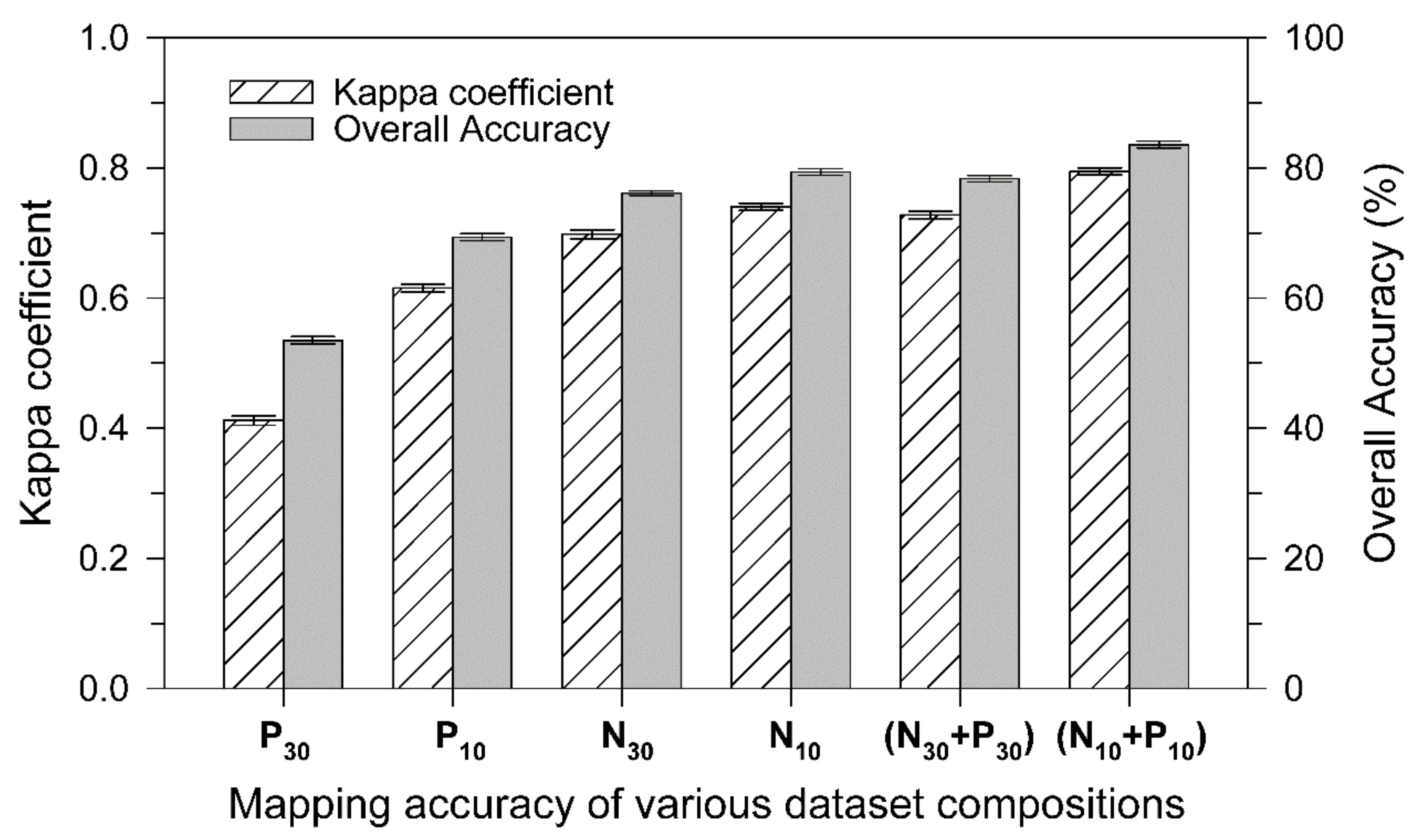
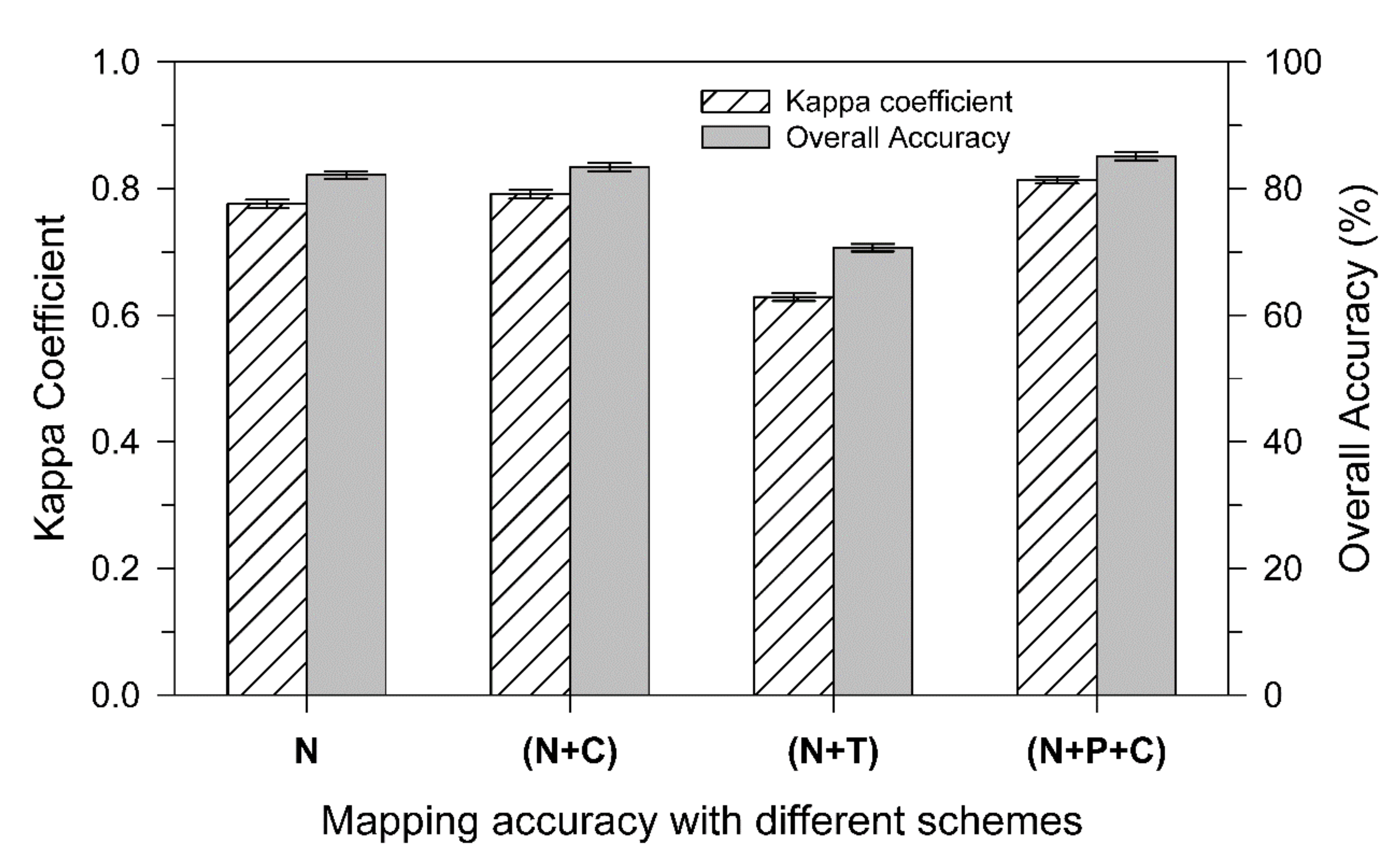
3.4. Forest Mapping on Landscape with Different Datasets

The landscape patterns based on SVM of different forest tree species in the study region combining with 10-day time series NDVI, the information of 22 PCs derived from PCA transformation based on 10-day NDVI, five phenological metrics, and contrast texture information showed that high spatial agreement occurred at intact forest area (Figure 9). The low spatial agreement was mainly dispersed at small and fragmented patches of tree species and the boundaries among different species. For the accuracy of forest mapping at landscape, there are only two tree species, Pt and Qm, with producer and user accuracies higher than 80% based on the original 10-day NDVI images, while the producer accuracy of Pd was lower than 53% (Table 3). The overall accuracy will reach over 82% when applied with NPCA and the producer and user accuracies of each tree species were higher than 70% (Table 3). The combination of NPCA and phenological metrics (P) would increase the overall accuracy to 83% and the accuracy of tree species identification had some enhancements. When the contrast was integrated with NPCA and phenological metrics, the accuracy of forested landscape identification increased to 85% and the producer (user) accuracies of each tree species identification could reach over 77.3% (81.5%) for Pd and 100% (92.4%) for Pt (Table 3). Regardless of the used data schemes, the producer (user) accuracies of each tree species revealed similar patterns, increasing from Pd to Bp, Lg, Qm to the best result of Pt (Table 3).

4. Discussion

The higher accuracies of forest mapping can usually be achieved by utilizing multi-temporal images instead of using a single one [82,83], and the seasonality of vegetation growth may be of critical assistance for separating land cover types [84]. Therefore, the high dimension of remotely sensed data will provide a better opportunity to capture the distinct cycles of annual growth of diverse vegetation [85,86]. In this study, we compared the effects of using different time-scale compositions derived from original 10-day GF-1 NDVI data on mapping tree species, and the results showed that the accuracy of tree species’ identification significantly increased from 30-day to 10-day time-series (p < 0.05). The accuracy of results was bettered when based on the PCA-transformed 10-day NDVI time series, by approximately 3%, because the PCA analysis can effectively remove redundant information from the time-series data and only retains a few independent spatiotemporal patterns that benefit forest identification [87,88].
The phenological metrics calculated from annual vegetation index has been proved to increase the capability of distinguishing the variance in different tree species [31], as well as the paddy rice area extraction [33]. Several studies revealed that there were still inconsistencies between land surface phenology obtained from remotely sensed data and in situ observations [30,89]. In our study, the SOS and EOS derived from time-series images of main studied tree species were identical to field data (Figure 4). This also explained why the accuracy of tree identification had significantly improved by integrating five phenological indicators derived from 10-day NDVI data instead of 30-day data. This finding also suggested that the relative lower resolution of data might miss the rapid seasonal shifts of vegetation growth [90,91].
Texture information, as a function of spatial patterns of pixel-spectral response in remotely sensed data, has been proved to improve forest mapping accuracy [53]. The study conducted in hinoki cypress and cool-temperate mixed forest based on six texture measures (homogeneity, contrast, dissimilarity, entropy, second moment and correlation) by GLCM derived from IKONOS-2 image in 4–20 m resolution indicated that the tree identification improved prominently, and kappa coefficient increased by 0.1 [34]. The relative work in the temperate forest in northeast China showed that the combination of four texture measures (contrast, entropy, second moment and correlation) by GLCM obtained from Gaofen images (1–8 m resolution) increased the power of discrimination of different tree species, Pinus tabulaeformis, Larix gmelinii, Populus davidiana, Betula platyphylla, and Quercus mongolica, by 2.0%, to 3.6% [36]. Although previous studies have confirmed the assistance of texture features to individual images, the effect of seasonal texture characteristics acquired from multi-temporal images remains highly uncertain. In this study, the comparisons indicated that the inclusion of CON, NDVI time series and phenological metrics significantly enhanced the accuracy of regional tree species identification. In the final landscape patterns of tree species identification, the highest accuracy of the scheme of NPCA+P+C also proved that, using this approach, the dispersal patterns of Populus davidiana (Pd) on flat valley in the study region and non-forest regions had been further decreased and eliminated (Figure 1 and Figure 9). However, we also found that the ENT, SM and COR served as input, in contrast, reduced the overall accuracy of the results by 12.7% which is the same as previous outcomes [55,56,57]. The commonly applied texture features, including contrast, correlation, and entropy, are demonstrated to be superior to using the entire texture features, in which the contrast (CON) was the most recommended [56]. Over-enhancement of the texture features would be contrary to leading to effective information loss and might consequently lower the capability of recognizing forest patterns [92].
In addition, the spatial resolution of the image has an important influence on the applicability of texture features [34,93]. Studies conducted on a single image suggested that including texture information would improve the accuracy of tree species identification when the spatial resolution was better than 36 m [34,94]. The spatial resolution (16 m) of GF-1 NDVI data utilized in this study is higher than studies suggested and has potential to obtain good quality detailed texture information [36,95]. Our study indicates that the higher spatiotemporal resolution utilized to map temperate forest tree species in northeast China performed competently. The tree species can be best recognized with a combination of 10-day NDVI time series, texture features, and phenological metrics, including multiple vegetation growth phases simultaneously, as mentioned [32,33]. With the advancement in higher spatiotemporal resolution of satellite images, it can be expected that the available data in the future will be more capable of mapping the forest tree species on landscape in more detail, with more conformity with ground truth. Furthermore, the development of a better strategy to precisely delineate the forest covers at landscape level is crucial to provide an accurate input to biogeochemical model for carbon, nutrient budgets and productivity estimations, and the following upscale simulations [96,97,98].
The further studies of tree identification are imperative for projected forest management in tropics and subtropics which provide diverse habitats for the wildlife and ecosystem services, and are also a vital carbon pool worldwide. It will be more challenging to map expected tree species in the humid tropical and subtropical regions where the more diverse evergreen broadleaved forests and mixed phenological cycles will make the identification of tree species complicated compared to temperate and arid regions. However, it will be valuable work for sustainable development.

5. Conclusions

With the increasing requirement to manage regional forest resources, it will be more fundamental to acquire the distribution of tree species in real-time. The time-series of satellite images provides spectral information of vegetation growth dynamics, which have a key role in identifying regional forest tree species. Compared to previous studies conducted with individual images, we proposed a method for identifying five dominant tree species on a forested landscape in northeast China based on time-series of remotely sensed data. The combination with a time-series of GF-1 NDVI images (10-day and 16 m in spatiotemporal resolution), the phenological metrics and temporal texture features of forest canopy, the kappa coefficient (overall accuracy) for the forest tree species can reach 0.814 (85.13%), which performed better than conventional monthly images. The free availability, better spatial resolution and wider coverage of GF-1 data compared to other environmental satellite images will have the potential for mapping tree species at a regional scale, and its application is also urgent in different forests with various environment settings.

Author Contributions

Conceptualization and Methodology, K.X.; Supervision, Q.T. and C.-T.C.; Software and Data Curation, Z.Z. and J.Y.; Writing—Original Draft, K.X.; Writing—Review and Editing, C.-T.C. and K.X.; Data collection and processing K.X. and J.Y. All authors have read and agreed to the published version of the manuscript.

Funding

This study was supported by grants from the Anhui Provincial Natural Science Foundation of China (Grant no. 2008085QD193); National Key R&D Program of China (Grant no. 2017YFD0600903); the Ministry of Science and Technology, Taiwan (MOST 105-2410-H-029-056-MY3, 108-2313-B-029-001).

Acknowledgments

Thanks to Huaifei Shen, Nianxu Xu and Shaofei Tang for the field work and data collection.

Conflicts of Interest

The authors declare no conflict of interest.

References

  1. Sannier, C.; McRoberts, R.E.; Fichet, L. Suitability of global forest change data to report forest cover estimates at national level in Gabon. Remote Sens. Environ. 2016, 173, 326–338. [Google Scholar] [CrossRef]
  2. Westoby, M. Selective forces exerted by vertebrate herbivores on plants. Trends Ecol. Evol. 1989, 4, 115–117. [Google Scholar] [CrossRef]
  3. Heinzel, J.; Koch, B. Investigating multiple data sources for tree species classification in temperate forest and use for single tree delineation. Int. J. Appl. Earth Obs. 2012, 18, 101–110. [Google Scholar] [CrossRef]
  4. Saatchi, S.; Buermann, W.; Ter Steege, H.; Mori, S.; Smith, T.B. Modeling distribution of Amazonian tree species and diversity using remote sensing measurements. Remote Sens. Environ. 2008, 112, 2000–2017. [Google Scholar] [CrossRef]
  5. Tang, L.N.; Shao, G.F. Drone remote sensing for forestry research and practices. J. For. Res. 2015, 26, 791–797. [Google Scholar] [CrossRef]
  6. Clark, M.L.; Roberts, D.A.; Clark, D.B. Hyperspectral discrimination of tropical rain forest tree species at leaf to crown scales. Remote Sens. Environ. 2005, 96, 375–398. [Google Scholar] [CrossRef]
  7. Wu, H.; Li, Z.L. Scale issues in remote sensing, a review on analysis, processing and modeling. Sensors 2009, 9, 1768–1793. [Google Scholar] [CrossRef]
  8. Fassnacht, F.E.; Latifi, H.; Stereńczak, K.; Modzelewska, A.; Lefsky, M.; Waser, L.T.; Straub, C.; Ghosh, A. Review of studies on tree species classification from remotely sensed data. Remote Sens. Environ. 2016, 186, 64–87. [Google Scholar] [CrossRef]
  9. Gessner, U.; Machwitz, M.; Conrad, C.; Dechab, S. Estimating the fractional cover of growth forms and bare surface in savannas. A multi-resolution approach based on regression tree ensembles. Remote Sens. Environ. 2013, 129, 90–102. [Google Scholar] [CrossRef] [Green Version]
  10. Latorre, A.P.; Cabezudo, B. Use of monocharacteristic growth forms and phenological phases to describe and differentiate plant communities in Mediterranean-type ecosystems. Plant Ecol. 2002, 161, 231–249. [Google Scholar] [CrossRef]
  11. Vilhar, U.; Skudnik, M.; Simončič, P. Phenological phases of trees on the intensive forest monitoring plots in slovenia. Acta Silvae Et Ligni 2013, 100, 5–17. [Google Scholar] [CrossRef] [Green Version]
  12. Almeida, J.; Dos Santos, J.A.; Alberton, B.; Morellato, L.P.C.; Ricardo, D.S.T. Plant species identification with phenological visual rhythms. In Proceedings of the IEEE International Conference on E-Science, Beijing, China, 22–25 October 2013. [Google Scholar] [CrossRef]
  13. Hill, R.A.; Wilson, A.K.; George, M.; Hinsley, S.A. Mapping tree species in temperate deciduous woodland using time-series multi-spectral data. Appl. Veg. Sci. 2010, 13, 86–99. [Google Scholar] [CrossRef]
  14. Jia, L.G.; Zhang, B.; Wei, H.D. The spectral characteristic variation analysis of three typical desert plants in growing season. Spectrosc. Spect. Anal. 2018, 38, 2881–2887. [Google Scholar] [CrossRef]
  15. Hoare, D.; Frost, P. Phenological description of natural vegetation in southern Africa using remotely-sensed vegetation data. Appl. Veg. Sci. 2004, 7, 19–28. [Google Scholar] [CrossRef]
  16. Tian, J.Q.; Zhu, X.L.; Wu, J.; Shen, M.G.; Chen, J. Coarse-resolution satellite images overestimate urbanization effects on vegetation spring phenology. Remote Sens. 2020, 12, 117. [Google Scholar] [CrossRef] [Green Version]
  17. Xiao, X.M.; Boles, S.; Liu, J.Y.; Zhuang, D.F.; Liu, M.L. Characterization of forest types in Northeastern China, using multi-temporal SPOT-4 VEGETATION sensor data. Remote Sens. Environ. 2002, 82, 335–348. [Google Scholar] [CrossRef]
  18. Kempeneers, P.; Sedano, F.; Seebach, L.M.; Strobl, P.; San-Miguel-Ayanz, J. Data fusion of different spatial resolution remote sensing images applied to forest-type mapping. IEEE T. Geocsi. Remote 2011, 49, 4977–4986. [Google Scholar] [CrossRef]
  19. Grabska, E.; Hostert, P.; Pflugmacher, D.; Ostapowicz, K. Forest stand species mapping using the Sentinel-2 time series. Remote Sens. 2019, 11, 1197. [Google Scholar] [CrossRef] [Green Version]
  20. Zhu, X.L.; Liu, D.S. Accurate mapping of forest types using dense seasonal Landsat time-series. ISPRS J. Photogramm. Remote Sens. 2014, 96, 1–11. [Google Scholar] [CrossRef]
  21. Puzzolo, V.; Denatale, F.; Gianne, F. Forest species discrimination in an Alpine mountain area using a fuzzy classification of multi-temporal SPOT (HRV) data. IEEE Int. Geosci. Remote Sens. Symp. 2003. [Google Scholar] [CrossRef]
  22. Persson, M.; Lindberg, E.; Reese, H. Tree species classification with multi-temporal Sentinel-2 data. Remote Sens. 2018, 10, 1794. [Google Scholar] [CrossRef] [Green Version]
  23. Wessel, M.; Brandmeier, M.; Tiede, D. Evaluation of different machine learning algorithms for scalable classification of tree types and tree species based on Sentinel-2 data. Remote Sens. 2018, 10, 1419. [Google Scholar] [CrossRef] [Green Version]
  24. Achard, F.; Estreguil, C. Forest classification of Southeast Asia using NOAA AVHRR data. Remote Sens. Environ. 1995, 54, 198–208. [Google Scholar] [CrossRef]
  25. Yui, X.F.; Zhuang, D.F.; Chen, H.; Hou, X.Y. Forest classification based on MODIS time series and vegetation phenology. In Proceedings of the IEEE International Geoscience and Remote Sensing Symposium (IGARSS), Anchorage, AK, USA, 20–24 September 2004; 2004. [Google Scholar] [CrossRef]
  26. Chang, B.H.; Wang, J.T.; Luo, Y.L.; Wang, Y.H.; Wang, Y.M. Cultivated land extraction based on GF-1/WFV remote sensing in Shenwu irrigation area of Hetao Irrigation District. Trans. Chin. Soc. Agric. Eng. 2017, 23, 188–195. [Google Scholar] [CrossRef]
  27. Liu, Y.Q.; Wang, L.; Zhao, X.N.; Qu, X.N.; Xu, X.; Wang, R. Extraction of crops in oasis based on GF-1/WFV time series. Arid Zone Res. 2019, 36, 781–789. [Google Scholar] [CrossRef]
  28. Roth, K.L.; Roberts, D.A.; Dennison, P.E.; Peterson, S.H.; Alonzo, M. The impact of spatial resolution on the classification of plant species and functional types within imaging spectrometer data. Remote Sens. Environ. 2015, 171, 45–57. [Google Scholar] [CrossRef]
  29. White, M.A.; de Beurs, K.M.; Didan, K.; Inouye, D.; Richardson, A.D.; Jensen, O.; O’Keefe, J.; Zhang, G.; Nemani, R.; van Leeuwen, W.J.D.; et al. Intercomparison, interpretation, and assessment of spring phenology in North America estimated from remote sensing for 1982–2006. Glob. Change Biol. 2009, 15, 2335–2359. [Google Scholar] [CrossRef]
  30. Ganguly, S.; Friedl, M.A.; Tan, B.; Zhang, X.Y.; Verma, M. Land surface phenology from MODIS: Characterization of the collection 5 global land cover dynamics product. Remote Sens. Environ. 2010, 114, 1805–1816. [Google Scholar] [CrossRef] [Green Version]
  31. Michez, A.; Piegay, H.; Jonathan, L.; Claessens, H.; Lejeune, P. Mapping of riparian invasive species with supervised classification of Unmanned Aerial System (UAS) imagery. Int. J. Appl. Earth Obs. 2015, 44, 88–94. [Google Scholar] [CrossRef]
  32. Kong, J.X.; Zhang, Z.C.; Zhang, J. Classification and identification of plant species based on multi-source remote sensing data: Research progress and prospect. Biodiv. Sci. 2019, 27, 796–812. [Google Scholar] [CrossRef]
  33. Liu, W.J.; Zeng, Y.N.; Zhang, M. Mapping rice paddy distribution by using time series HJ blend data and phenological parameters. J. Remote Sens. 2018, 22, 381–391. [Google Scholar] [CrossRef]
  34. Ota, T.; Mizoue, N.; Yoshida, S. Influence of using texture information in remote sensed data on the accuracy of forest type classification at different levels of spatial resolution. J. For. Res. 2011, 16, 432–437. [Google Scholar] [CrossRef]
  35. Li, M.Y.; Xing, Y.Q.; Liu, M.S.; Wang, Z.; Yao, S.T.; Zeng, X.J.; Xie, J. Identification of forest type with Landsat-8 image based on SVM. J. Cent. S. Univ. For. Technol. 2017, 37, 52–58. [Google Scholar] [CrossRef]
  36. Xu, K.J.; Tian, Q.J.; Yue, J.B.; Tang, S.F. Forest tree species identification and its response to spatial scale based on multispectral and multi-resolution remotely sensed data. Chin. J. Appl. Ecol. 2018, 29, 3986–3994. [Google Scholar] [CrossRef]
  37. Ke, S.F.; Li, B.; Yang, Y.H.; Ma, C.G.; Jia, Y.S. The evaluation of carbon footprint from the operation of forest farm and carbon storage by forest resources based on the Wangyedian forest farm in Chifeng of Inner Mongolia. For. Econ. 2013, 35, 93–101. [Google Scholar] [CrossRef]
  38. Gong, P.; Pu, R.L.; Yu, B. Conifer species recognition with seasonal hyperspectral data. J. Remote Sens. 1998, 2, 211–217. [Google Scholar] [CrossRef]
  39. Zheng, B.; Myint, S.W.; Thenkabail, P.S.; Aggarwal, R.M. A support vector machine to identify irrigated crop types using time-series Landsat NDVI data. Int. J. Appl. Earth Obs. 2015, 34, 103–112. [Google Scholar] [CrossRef]
  40. Estoque, R.C.; Murayama, Y.; Akiyama, C.M. Pixel-based and object-based classifications using high- and medium-spatial-resolution imageries in the urban and suburban landscapes. Geocarto Int. 2015, 30, 1113–1129. [Google Scholar] [CrossRef] [Green Version]
  41. Xu, K.; Tian, Q.; Yang, Y.; Yue, J.; Tang, S. How up-scaling of remote-sensing images affects land-cover classification by comparison with multiscale satellite images. Int. J. Remote Sens. 2019, 40, 2784–2810. [Google Scholar] [CrossRef]
  42. Yang, Y.; Tao, B.; Ren, W.; Zourarakis, D.P.; Masri, B.E.; Sun, Z.; Tian, Q. An improved approach considering intraclass variability for mapping winter wheat using multitemporal MODIS EVI images. Remote Sens. 2019, 11, 1191. [Google Scholar] [CrossRef] [Green Version]
  43. Xu, K.J.; Zeng, H.D.; Zhu, X.B.; Tian, Q.J. Evaluation of five commonly used atmospheric correction algorithms for multi-temporal aboveground forest carbon storage estimation. Spectrosc. Spect. Anal. 2017, 37, 3493–3498. [Google Scholar] [CrossRef]
  44. Huete, A.; Didan, K.; Miura, T.; Rodriguez, E.P.; Gao, X.; Ferreira, G. Overview of the radiometric and biophysical performance of the MODIS vegetation indices. Remote Sens. Environ. 2002, 83, 195–213. [Google Scholar] [CrossRef]
  45. Birky, A.K. NDVI and a simple model of deciduous forest seasonal dynamics. Ecol. Model. 2001, 143, 43–58. [Google Scholar] [CrossRef]
  46. Hird, J.N.; Mcdermid, G.J. Noise reduction of NDVI time series: An empirical comparison of selected techniques. Remote Sens. Environ. 2009, 113, 248–258. [Google Scholar] [CrossRef]
  47. Chen, J.; Jönsson, P.; Tamura, M.; Gu, Z.; Matsushita, B.; Eklundh, L. A simple method for reconstructing a high-quality NDVI time-series data set based on the Savitzky–Golay filter. Remote Sens. Environ. 2004, 91, 332–344. [Google Scholar] [CrossRef]
  48. Wang, Y.F.; Xue, Z.H.; Chen, J.; Chen, G.Z. Spatio-temporal analysis of phenology in Yangtze river delta based on MODIS NDVI time series from 2001 to 2015. Front. Earth Sci-Prc. 2019, 13, 92–110. [Google Scholar] [CrossRef]
  49. Li, R.; Zhang, X.; Liu, B.; Zhang, B. Review on methods of remote sensing time-series data reconstruction. J. Remote Sens. 2009, 13, 335–341. [Google Scholar] [CrossRef]
  50. Zhao, G.; Maclean, A.L. A comparison of canonical discriminant analysis and principal component analysis for spectral transformation. Photogramm. Eng. Rem. Sens. 2000, 66, 841–847. [Google Scholar] [CrossRef]
  51. Alessandri, A.; Navarra, A. On the coupling between vegetation and rainfall inter-annual anomalies: Possible contributions to seasonal rainfall predictability over land areas. Geophys. Res. Lett. 2008, 35, L02718. [Google Scholar] [CrossRef]
  52. Chang, C.T.; Wang, H.C.; Huang, C. Retrieving multi-scale climatic variations from high dimensional time-series MODIS green vegetation cover in a tropical/subtropical mountains island. J. Mt. Sci. 2014, 11, 407–420. [Google Scholar] [CrossRef]
  53. Coburn, C.A.; Roberts, A.C.B. A multiscale texture analysis procedure for improved forest stand classification. Int. J. Remote Sens. 2004, 25, 4287–4308. [Google Scholar] [CrossRef] [Green Version]
  54. Dutta, S.; Datta, A.; Chakladar, N.D.; Pal, S.K.; Mukhopadhyay, S.; Sen, R. Detection of tool condition from the turned surface images using an accurate grey level co-occurrence technique. Precis. Eng. 2012, 36, 458–466. [Google Scholar] [CrossRef]
  55. Franklin, S.E.; Hall, R.J.; Moskal, L.M.; Maudie, A.J.; Lavigne, M.B. Incorporating texture into classification of forest species composition from airborne multispectral images. Int. J. Remote Sens. 2000, 21, 61–79. [Google Scholar] [CrossRef]
  56. Clausi, D.A. An analysis of co-occurrence texture statistics as a function of grey level quantization. Can. J. Remote Sens. 2002, 28, 45–62. [Google Scholar] [CrossRef]
  57. Gallardo-Cruz, J.A.; Meave, J.A.; González, E.J.; Lebrija-Trejos, E.E.; Romero-Romero, M.A.; Pérez-García, E.A.; Gallardo-Cruz, R.; Hernández-Stefanoni, J.L.; Martorell, C. Predicting tropical dry forest successional attributes from space, is the key hidden in image texture. PLoS ONE 2012, 7, e30506. [Google Scholar] [CrossRef] [Green Version]
  58. Wang, G.X.; Gertner, G.; Anderson, A.B. Up-scaling methods based on variability–weighting and simulation for inferring spatial information across scales. Int. J. Remote Sens. 2004, 25, 4961–4979. [Google Scholar] [CrossRef]
  59. Kayitakire, F.; Hamel, C.; Defourny, P. Retrieving forest structure variables based on image texture analysis and IKONOS-2 imagery. Remote Sens. Environ. 2006, 102, 390–401. [Google Scholar] [CrossRef]
  60. Haralick, R.M.; Shanmugam, K.; Dinstein, I. Textural features for image classification. IEEE Trans. Syst. Man. Cybern. 1973, 3, 610–621. [Google Scholar] [CrossRef] [Green Version]
  61. Niel, T.G.V.; Mcvicar, T.R.; Datt, B. On the relationship between training sample size and data dimensionality: Monte Carlo analysis of broadband multi-temporal classification. Remote Sens. Environ. 2005, 98, 468–480. [Google Scholar] [CrossRef]
  62. Wang, C.Y.; Liu, Z.J.; Yan, C.Y. A experimental study on imaging spectrometer data feature selection and wheat type identification. J. Remote Sens. 2006, 10, 249–255. [Google Scholar] [CrossRef]
  63. Adam, E.; Mutanga, O. Spectral discrimination of papyrus vegetation (Cyperus papyrus L.) in swamp wetlands using field spectrometry. ISPRS J. Photogramm. Remote Sens. 2009, 64, 612–620. [Google Scholar] [CrossRef]
  64. Tottrup, C.; Rasmussen, M.S.; Eklundh, L. Mapping fractional forest cover across the highlands of mainland Southeast Asia using MODIS data and regression tree modelling. Int. J. Remote Sens. 2007, 28, 23–46. [Google Scholar] [CrossRef]
  65. Seaquist, J.W.; Hickler, T.; Eklundh, L. Disentangling the effects of climate and people on Sahel vegetation dynamics. Biogeosciences 2009, 6, 469–477. [Google Scholar] [CrossRef]
  66. Jönnson, P.; Eklundh, L. TIMESAT-a program for analyzing time-series of satellite sensor data. Comput. Geosci. 2004, 30, 833–845. [Google Scholar] [CrossRef] [Green Version]
  67. Chang, C.T.; Wang, H.C.; Huang, C. Impact of vegetation onset time on the net primary productivity in a mountainous island in Pacific Asia. Environ. Res. Lett. 2013, 8, 045030. [Google Scholar] [CrossRef] [Green Version]
  68. Yang, Y.T.; Guan, H.D.; Shen, M.G.; Liang, W.; Jiang, L. Changes in autumn vegetation dormancy onset date and the climate controls across temperate ecosystems in China from 1982 to 2010. Glob. Change Biol. 2014, 21, 1–14. [Google Scholar] [CrossRef]
  69. Beck, P.S.A.; Atzberger, C.; Høgda, K.A.; Johansen, B.; Skidmore, A.K. Improved monitoring of vegetation dynamics at very high latitudes: A new method using MODIS NDVI. Remote Sens. Environ. 2006, 100, 321–334. [Google Scholar] [CrossRef]
  70. Heumann, B.W.; Seaquist, J.W.; Eklundh, L.; Jönsson, P. AVHRR derived phenological change in the Sahel and Soudan, Africa, 1982–2005. Remote Sens. Environ. 2007, 108, 385–392. [Google Scholar] [CrossRef]
  71. Jiao, F.S.; Liu, H.Y.; Xu, X.J.; Gong, H.B.; Lin, Z.S. Trend evolution of vegetation phenology in China during the period of 1981–2016. Remote Sens. 2020, 12, 572. [Google Scholar] [CrossRef] [Green Version]
  72. Zhao, S.H.; Feng, X.Z.; Du, J.K.; Lin, G.F. SPIN-2 panchromatic and SPOT-4 multi-spectral image fusion based on support vector machine. J. Remote Sens. 2003, 7, 407–411. [Google Scholar] [CrossRef]
  73. Dalponte, M.; Bruzzone, L.; Gianelle, D. Fusion of hyperspectral and LIDAR remote sensing data for classification of complex forest areas. IEEE Trans. Geosci. Remote. 2008, 46, 1416–1427. [Google Scholar] [CrossRef] [Green Version]
  74. Bruzzone, L.; Persello, C. A novel context-sensitive semi-supervised SVM classifier robust to mislabeled training samples. IEEE Trans. Geosci. Remote. 2009, 47, 2142–2154. [Google Scholar] [CrossRef] [Green Version]
  75. Shao, Y.; Lunetta, R.S. Comparison of support vector machine, neural network, and CART algorithms for the land-cover classification using limited training data points. ISPRS J. Photogramm. 2012, 70, 78–87. [Google Scholar] [CrossRef]
  76. Kumar, P.; Gupta, D.K.; Mishra, V.N.; Prasad, R. Comparison of support vector machine, artificial neural network, and spectral angle mapper algorithms for crop classification using LISS IV data. Int. J. Remote Sens. 2015, 36, 1604–1617. [Google Scholar] [CrossRef]
  77. Raczko, E.; Zagajewski, B. Comparison of support vector machine, random forest and neural network classifiers for tree species classification on airborne hyperspectral APEX images. Eur. J. Remote Sens. 2017, 50, 144–154. [Google Scholar] [CrossRef] [Green Version]
  78. Thanh-Noi, P.; Kappas, M. Comparison of random forest, k-nearest neighbor, and support vector machine classifiers for land cover classification using Sentinel-2 imagery. Sensors 2018, 18, 18. [Google Scholar] [CrossRef] [Green Version]
  79. Kuemmerle, T.; Radeloff, V.C.; Perzanowski, K.; Hostert, P. Cross-border comparison of land cover and landscape pattern in eastern Europe using a hybrid classification technique. Remote Sens. Environ. 2006, 103, 449–464. [Google Scholar] [CrossRef]
  80. Sothe, C.; de Almeida, C.M.; Liesenberg, V.; Schimalski, M.B. Evaluating Sentinel-2 and Landsat-8 data to map sucessional forest stages in a subtropical forest in southern Brazil. Remote Sens. 2017, 9, 838. [Google Scholar] [CrossRef] [Green Version]
  81. Janssen, L.L.F.; van de Rwel, F.J.M. Accuracy assessment of satellite derived land-gover data: A review. Photogramm. Eng. Rem. S. 1994, 60, 419–426. [Google Scholar] [CrossRef]
  82. Madonsela, S.; Cho, M.A.; Mathieu, R.; Mutanga, O.; Ramoelo, A.; Kaszta, Ż.; van de Kerchove, R.; Wolff, E. Multi-phenology WorldView-2 imagery improves remote sensing of savannah tree species. Int. J. Appl. Earth Obs. 2017, 58, 65–73. [Google Scholar] [CrossRef] [Green Version]
  83. Xie, Z.L.; Chen, Y.L.; Lu, D.S.; Li, G.Y.; Chen, R.X. Classification of land cover, forest, and tree species classes with ZiYuan-3 multispectral and stereo data. Remote Sens. 2019, 11, 164. [Google Scholar] [CrossRef] [Green Version]
  84. Mannel, S.; Price, M. Comparing classification results of multi-seasonal TM against AVIRIS imagery – seasonality more important than number of bands. Photogramm. Fernerkun. 2012, 2012, 603–612. [Google Scholar] [CrossRef]
  85. Immitzer, M.; Vuolo, F.; Atzberger, C. First experience with Sentinel-2 data for crop and tree species classifications in Central Europe. Remote Sens. 2016, 8, 166. [Google Scholar] [CrossRef]
  86. Vuolo, F.; Neuwirth, M.; Immitzer, M.; Atzberger, C.; Ng, W.T. How much does multi-temporal Sentinel-2 data improve crop type classification? Int. J. Appl. Earth Obs. 2018, 72, 122–130. [Google Scholar] [CrossRef]
  87. Zhang, J.K.; Rivard, B.; Sánchez-Azofeifa, A.; Castro-Esau, K. Intra- and inter- class spectral variability of tropical tree species at La Selva, Costa Rica, Implications for species identification using HYDICE imagery. Remote Sens. Environ. 2006, 105, 129–141. [Google Scholar] [CrossRef]
  88. Chakravorty, R.; Gauri, S.K.; Chakravorty, S. A modified principal component analysis-based utility theory approach for optimization of correlated responses of EDM process. Int. J. Technol. Manag. 2012, 4, 34–45. [Google Scholar] [CrossRef] [Green Version]
  89. Moulin, S.; Kergoat, L.; Viovy, N.; Dedieu, G. Global-scale assessment of vegetation phenology using NOAA/AVHRR satellite measurements. J. Clim. 1997, 10, 1154–1170. [Google Scholar] [CrossRef]
  90. Ahl, D.E.; Gower, S.T.; Burrows, S.N.; Shabanov, N.V.; Myneni, R.B.; Knyazikhin, Y. Monitoring spring canopy phenology of a deciduous broadleaf forest using MODIS. Remote Sens. Environ. 2006, 104, 88–95. [Google Scholar] [CrossRef] [Green Version]
  91. Zhang, X.; Friedl, M.A.; Schaaf, C.B. Sensitivity of vegetation phenology detection to the temporal resolution of satellite data. Int. J. Remote Sens. 2009, 30, 2061–2074. [Google Scholar] [CrossRef]
  92. Luo, L.L.; Wang, X.X.; Nong, J.H.; Liang, Z.J.; Tang, G.Y. Remote sensing forest classification with texture based on ICA and SVM. Comput. Eng. Appl. 2012, 48, 227–229. [Google Scholar] [CrossRef]
  93. Pu, R.L.; Landry, S. A comparative analysis of high spatial resolution IKONOS and WorldView-2 imagery for mapping urban tree species. Remote Sens. Environ. 2012, 124, 516–533. [Google Scholar] [CrossRef]
  94. Kushwaha, S.P.S.; Kuntz, S.; Oesten, G. Applications of image texture in forest classification. Int. J. Remote Sens. 1994, 15, 2273–2284. [Google Scholar] [CrossRef]
  95. Wulder, M.A.; LeDrew, E.F.; Franklin, S.E.; Lavigne, M.B. Aerial image texture information in the estimation of northern deciduous and mixed wood forest leaf area index (LAI). Remote Sens. Environ. 1998, 64, 64–76. [Google Scholar] [CrossRef]
  96. Pietsch, S.A.; Hasenauer, H.; Thornton, P.E. BGC-model parameters for tree species growing in central European forests. For. Ecol. Manag. 2005, 211, 264–295. [Google Scholar] [CrossRef]
  97. Liu, J.; Liu, S.; Loveland, T.R.; Tieszen, L.L. Integrating remotely sensed land cover observations and a biogeochemical model for estimating forest ecosystem carbon dynamics. Ecol. Model. 2008, 219, 361–372. [Google Scholar] [CrossRef]
  98. Keller, A.B.; Reed, S.C.; Townsend, A.R.; Cleveland, C.C. Effects of canopy tree species on belowground biogeochemistry in a lowland wet tropical forest. Soil Biol. Biochem. 2013, 58, 61–69. [Google Scholar] [CrossRef]
Figure 1. The geographical location map of the study region and major vegetation cover types in background (a,b), and the sampling sites of five tree species, including evergreen coniferous forest dominated by Pinus tabulaeformis (Pt), deciduous coniferous forest dominated by Larix gmelinii (Lg), and three deciduous broadleaved forest dominated by Quercus mongolica (Qm), Betula platyphylla (Bp), and Populus davidiana (Pd), (n = 1650, approximately 330 for each tree species) overlaid on a GF-1 image (22 August 2017) in background (c).
Remotesensing 12 01554 g001
Figure 2. The canopy images of five dominant tree species taken by unmanned aerial vehicle (UAV) during the summer of 2017 in the study region (upper panels), and the vertical structure of forest stand (bottom panels). The abbreviations of Pt (a), Lg (b), Qm (c), Bp (d), and Pd (e) stand for Pinus tabulaeformis, Larix gmelinii, Quercus mongolica, Betula platyphylla, and Populus davidiana, respectively.
Remotesensing 12 01554 g002
Figure 3. The working flow of major images acquired, data processing, texture feature extractions, phenologiocal metrics calculation, and landscape mapping and accuracy assessment in ENVI and ArcGIS software.
Remotesensing 12 01554 g003
Figure 4. The differences of the start of growing season (SOS) (a) and the end of growing season (EOS) (b) between observations and time setting on fitting curve of NDVI time series in TIMESAT. Four deciduous tree species in the study area include Larix gmelinii (Lg), Quercus mongolica (Qm), Betula platyphylla (Bp), and Populus davidiana (Pd), except for Pinus tabulaeformis (Pt) without in-situ records.
Remotesensing 12 01554 g004
Figure 5. The identification accuracy of dominant tree species based on NDVI time series data of different temporal scales (a), and the eigenvalues of principal component analysis (PCA) based on 10-day NDVI time series, and the kappa coefficient and overall accuracy (OA) of dominant tree species identifications considering the number of PCs in the analysis (b).
Remotesensing 12 01554 g005
Figure 6. The landscape patterns of five phenological metrics in study region, the SOS (start of growing season, Julian date), EOS (end of growing season, Julian date), LOS (length of season, days), POS (peak of growing season, Julian date), and LOP (length of peak, days) from the top to bottom respectively (a), and the comparisons of SOS, EOS, LOS, POS, and LOP among five tree species (Pt, Lg, Qm, Bp, and Pd) from the top to bottom (b). The five metrics are significant different among various species (p < 0.05).
Remotesensing 12 01554 g006
Figure 7. The kappa coefficient and overall accuracy of forest tree species identification based on different time series NDVI images, phenological metrics and different schemes of combinations of NDVI and phenological metrics. The P30 and P10 indicates phenological metrics obtained from 30-day and 10-day images, and N30 and N10 stand for time series of 30-day and 10-day NDVI time series respectively.
Remotesensing 12 01554 g007
Figure 8. The kappa coefficient and overall accuracy of tree species mapping using different schemes including 10-day NDVI time series images (N), four texture parameters (T), five phenological metrics (P) and contrast (C) of texture feature.
Remotesensing 12 01554 g008
Figure 9. The landscape patterns of tree species identification for study area based on individual and combinations of datasets including (a) N, (b) NPCA, (c) NPCA+P, and (d) NPCA+P+C. N indicates the 10-day time series NDVI data without PCA transform, NPCA stands for 22 PCs derived from PCA transformation based on 10-day NDVI, P indicates the five phenological metrics derived from 10-day NDVI images, and C means the contrast of texture feature.
Remotesensing 12 01554 g009
Table 1. The information of satellite images used in this study.
NumberAcquisition DateNumberAcquisition DateNumberAcquisition Date
12017011013201705072520170921
22017011814201705202620170930
32017020215201705292720171014
42017021116201706102820161019
52017021917201706262920161023
62017022818201707083020171103
72017030819201707173120171116
82017031220201708103220171124
92017032521201708223320171202
102017040922201708303420171215
112016042223201709073520171223
122017043024201709123620171231
Table 2. The J-M distance among different forest tree species. The abbreviations of Pt, Lg, Qm, Bp, and Pd stand for tree species Pinus tabulaeformis, Larix gmelinii, Quercus mongolica, Betula platyphylla, and Populus davidiana respectively.
Pair-ComparisonsCONENTSMCOR
Pt - Lg1.9895 1.6694 1.7974 1.4946
Pt - Qm2.0000 1.9698 1.9848 1.9299
Pt - Bp1.9995 1.8105 1.9046 1.7102
Pt - Pd2.0000 1.9968 1.9998 1.9707
Lg - Qm2.0000 1.9489 1.9737 1.9305
Lg - Bp1.9989 1.5586 1.6454 1.4655
Lg - Pd2.0000 1.9860 1.9997 1.9529
Qm - Bp1.9991 1.9622 1.9830 1.9504
Qm - Pd2.0000 1.9962 1.9999 1.9875
Bp - Pd 2.0000 1.9974 2.0000 1.9778
Table 3. Producer’s accuracy (PA) and user’s accuracy (UA) of forest mapping for individual tree species and overall accuracy based on different schemes. N indicates the original 10-day NDVI time series, NPCA stands for transformed patterns of 22 PCs from PCA analysis based on 10-day time series of NDVI, P indicates the phenological metrics derived from 10-day NDVI images, and C means the contrast of texture feature.
SchemesNNPCANPCA+PNPCA+P+C
AccuracyPAUAPAUAPAUAPAUA
Pt99.1892.0296.7293.6510091.6710092.4
Lg77.9576.2178.8777.7078.7079.7480.4381.86
Qm80.4983.7685.1585.5784.2489.0184.9889.23
Bp78.8870.6677.8375.2182.4677.3781.9480.17
Pd52.9171.0970.0577.9870.7779.3177.3281.52
Overall accuracy 79.4082.1883.6285.13

