Abstract
Observing global terrestrial water storage changes (TWSCs) from (inter-)seasonal to (multi-)decade time-scales is very important to understand the Earth as a system under natural and anthropogenic climate change. The primary goal of the Gravity Recovery And Climate Experiment (GRACE) satellite mission (2002–2017) and its follow-on mission (GRACE-FO, 2018–onward) is to provide time-variable gravity fields, which can be converted to TWSCs with km spatial resolution; however, the one year data gap between GRACE and GRACE-FO represents a critical discontinuity, which cannot be replaced by alternative data or model with the same quality. To fill this gap, we applied time-variable gravity fields (2013–onward) from the Swarm Earth explorer mission with low spatial resolution of km. A novel iterative reconstruction approach was formulated based on the independent component analysis (ICA) that combines the GRACE and Swarm fields. The reconstructed TWSC fields of 2003–2018 were compared with a commonly applied reconstruction technique and GRACE-FO TWSC fields, whose results indicate a considerable noise reduction and long-term consistency improvement of the iterative ICA reconstruction technique. They were applied to evaluate trends and seasonal mass changes (of 2003–2018) within the world’s 33 largest river basins.
1. Introduction
The Gravity Recovery And Climate Experiment (GRACE, 2002–2017) satellite mission [1] was a joint United States (National Aeronautics and Space Administration, NASA) and German (Deutsche Zentrum für Luft- und Raumfahrt, DLR) space mission, which provided estimates of variations in the gravity field arising from mass movements within the Earth system. GRACE was launched on 17th March 2002, and consisted of two identical spacecraft, one following the other, in the same orbit separated by roughly 220 km. The variations in the distance between the two GRACE satellites were measured by a K/Ka-Band Ranging (KBR) system, which can largely be attributed to global mass changes within the Earth’s interior, at its surface, and in the atmosphere.
Over any typical 30-day span (the nominal data accumulation interval of GRACE gravity field solutions) of the non-repeating orbit configurations, a dense ground track grid can be obtained (see e.g., [2]); therefore, usually (almost) one month of the pre-processed GRACE along-track KBR data were used to compute time-variable gravity field solutions that are known as the GRACE level 2 data (GRACE L2, [3]). These L2 data were used to provide satellite-based estimates of global and regional terrestrial water storage change (TWSC, a vertical summation of water storage changes) with a few hundred kilometers spatial resolution, e.g., over Asia (e.g., [4,5,6]), Africa (e.g., [7,8]), and Australia (e.g., [9,10,11]). On a global scale, TWSCs are discussed, e.g., in [12,13,14,15,16]. All these studies came to the same conclusion that GRACE L2 products are suitable for studying large scale TWSCs on decadal, annual, and inter-annual time scales. A review of GRACE applications in climate studies is provided in [17].
Initially, GRACE was targeted to cover a five-year period, which was exceeded by ten years till October 2017. The GRACE Follow-On (GRACE-FO, [18]) mission was launched in May 2018, but suffered a failure of the main instrument processing unit between July and October 2018. This has led to approximately one year of data gap. Many studies have been working to bridge the gap between GRACE and GRACE-FO missions using alternative observations. However, there is no single satellite mission or proxy observation which is able to fill this gap with comparable quality (see e.g., [19,20,21]).
Geodetic satellite laser ranging (SLR) is another geodetic remote sensing observation technique that provides information about temporal variations of the Earth’s gravity field at the lowest degrees of the spherical harmonic spectrum (e.g., up to degree and order 6), and covers a longer time series than GRACE mission (see e.g., [22,23,24,25,26]). The long time span of collecting data by SLR missions provides an opportunity to determine the Earth’s gravity field before GRACE and during the gap between GRACE and GRACE-FO. Talpe et al. [27] combined high-resolution gravity fields derived from GRACE with the low-resolution fields from SLR/DORIS (Doppler Orbitography and Radiopositioning Integrated by Satellite, DORIS) tracking data, to reconstruct global time-variable gravity fields for the period of 1993–2013. In [28], GRACE observations were combined with SLR data to reconstruct a consistent long-term estimation of the Earth’s gravity field.
In addition to GRACE and SLR missions, satellites in low earth orbit (LEO), namely the European Space Agency (ESA)’s Swarm Earth explorer mission, provides Earth gravity field models from alternative sources of gravimetric data. Swarm consists of three identical satellites (launched on 22 November 2013) [29], where two satellites are orbiting the Earth side-by-side in nearly polar orbits currently (November 2019) at the altitude of ∼ 430 km (Swarm-Alpha and Swarm-Charlie, separated by 15 s in time at their equatorial crossing) and one is flying at higher altitude of ∼ 500 km (Swarm-Bravo). Swarm’s main mission objective is to measure the Earth’s magnetic field; however, since the Swarm satellites are equipped with geodetic-quality GPS receivers, accelerometers, star-tracker assemblies, and laser retro-reflectors, their high-low satellite-to-satellite tracking (hl-SST) observing system provides the opportunity of computing time-variable gravity field solutions as shown by [30,31], and [21]. Recently, [32] provided a long-term time series of monthly gravity field solutions as a combination of SLR data, GPS and K/Ka-band observations of the GRACE mission, and GPS observations of the three Swarm satellites. In their study the monthly gravity field derived from Swarm were used to fill the gap between GRACE and GRACE-FO missions.
GRACE L2 data are provided up to degree and order 96 [33]. Since the fields are noisy, isotropic (e.g., Gaussian in [34]), or anisotropic and de-striping or decorrelation filters (e.g., [35,36,37,38], with ∼ 300–900 km half radius based on the application) have often been applied to achieve TWSC fields of few hundred km resolution. Swarm’s monthly gravity fields, in contrast, have been computed up to degree and order 70, but contain significant time-variable signal only up to about degree 13 (∼1500 km or longer resolution), and the fields are relatively noisy [39], where filters with the smoothing radius between 500–833 km were used to estimate TWSC fields with few thousand km resolution [39]. This fact limits the application of Swarm data for, e.g., continental hydrology, where higher resolution estimations are desirable [40]; therefore, improving the spatial resolution and reducing the level of noise in Swarm fields are required to enhance their application for hydrological applications. This topic is addressed in this study.
In order to fill the gap between GRACE and GRACE-FO, in a recent study, [41] developed an empirical approach to predict GRACE-like TWSC fields using the climate inputs as indicators. Their study addresses the prediction of TWSC in large river basins but it is restricted to the regions that contain high correlation between climate variations and water storage changes. The empirical technique that they applied also requires a learning phase that might be relatively sensitive to the episodic variations caused by natural (e.g., floods and droughts) and anthropogenic factors (e.g., water storage over extractions).
In this study, two reconstruction formulations (Approach 1 and Approach 2) are proposed, which can be used to merge GRACE and Swarm time-variable gravity fields. The proposed approach of this study entirely relies on gravity field outputs, which can be derived from different satellite missions. For both formulations, one can apply statistical decomposition techniques such as principal component analysis (PCA, [42]) and independent component analysis (ICA, [13,43]) or their extensions (Complex PCA and Complex ICA, as in [44]). Here, we prefer ICA over PCA, since it performs better to separate TWSC signal from noise (see, e.g., [45,46]). Besides, ICA’s independent modes can better be related to physical phenomena as shown by e.g., [9,13,47]. Approach 1 follows a common data reconstruction procedure similar to [27,48], but in the spatial grid domain (TWSC), although Approach 2 is novel and formulated as an iterative ICA-based reconstruction, using the whole period of available GRACE and Swarm TWSC time series, covering 2003–2018.
Validating GRACE TWSC fields was performed by comparisons with geophysically relevant signals from independent data sources. For example, hydrological models were used to assess GRACE data over land area (e.g., [9,49]); however, many studies, e.g., [16,50], indicate that the trend and seasonality of these models are uncertain and such comparisons might be performed with care. Other studies, e.g., [51,52,53] suggested the use of in-situ data such as ocean bottom pressure and global navigation satellite systems (GNSS)-derived vertical loads to assess GRACE signals. These validations are more suited to evaluate low degree spectral (long wavelength spatial) variations. Over (large) lakes, satellite altimetry and in-situ data can be used to assess GRACE data; however, a reliable reduction of hydrological signals surrounding these lakes is a challenging task (see, e.g., [54,55,56]). In this study, satellite altimetry data over selected lakes are used as an indicator of changes in trend and/or seasonality of TWSCs derived from the reconstructed data. In addition, TWSCs derived from GRACE-FO is used to evaluate the reconstructed TWSC in this study, for some selected months after the year 2018.
In what follows, data sources of this study are described in Section 2, and the two alternative reconstruction techniques are formulated in Section 3. Our goal was to illustrate that the optimal combination of the GRACE and Swarm (three-satellite constellation) temporal gravity field solutions improves the resulting retrieved TWSC fields compared with mass estimation from only one type of satellite mission pleonastic. In Section 4, the main results of this study are presented including a comparison between the two approaches used for reconstruction, an evaluation of the reconstructed TWSCs in comparison with that of the GRACE-FO product, as well as an evaluation of mass changes (2003–2018) within the world’s 33 major river basins. Finally in Section 5, the main conclusions and an outlook are provided. This paper has two appendices that provide detailed information about the efficiency of the presented reconstruction approach in decreasing the level of noise and spatial leakage in GRACE and Swarm data.
2. Data
In this section, satellite geodetic data to be used to estimate global TWSC fields and their post-processing are described.
2.1. GRACE L2 Fields
The GRACE mission consists of two identical spacecraft (GRACE-A and GRACE-B) following each other in tandem in a single orbital plane. The twins are equipped with a K/Ka-band ranging system (KBR) to provide inter-satellite ranges. In addition, both satellites carry GPS receivers that are used for orbit determination, as well as accelerometers to remove non-gravitational forces prior to gravity modeling. The time-variable GRACE gravity field solutions, known as GRACE level 2 (L2) products, are provided by a number of institutions, using different processing approaches, background models, and assumptions.
For this study, the latest release of monthly GRACE L2 product (RL06, [57]), covering April 2002 to September 2016, and the previous release (RL05), covering November 2016 to January 2017, expressed as spherical harmonic coefficients up to degree and order 96, were downloaded from the Center for Space Research (CSR, http://www2.csr.utexas.edu/grace/). The biases between RL05 and RL06 data will be eliminated by implementing the reconstruction procedure introduced in Section 3. To evaluate the reconstruction results of this, GRACE-FO data of 2019 were downloaded from the CSR website. It is worth noting here that, due to the aging batteries on the GRACE satellites, no ranging data were collected during certain orbit periods, and hence no gravity fields could be computed. These gaps occur approximately every 5–6 months, mostly after 2011, and last for 4–5 weeks. The months with no GRACE data are June and July 2002, June 2003, January and June 2011, May and October 2012, March, August and September 2013, February, July, and December 2014, June, October, and November 2015, April, September, and October in 2016.
2.2. Swarm L2 Gravity Field Models
The three satellites of ESA’s Earth’s Magnetic Field and Environment Explorer (Swarm) mission, which were launched in November 2013, were designed specifically to accurately measure the Earth’s magnetic and electric fields [29]. Global positioning satellite (GPS) receiver, one aboard each Swarm satellite, allows them to produce precise orbit solutions accurate to centimeters in conjunction with post processing of the orbital data using gravity field models [58].
The Swarm level 1b products (processed raw satellite measurements) are released by ESA to represent the best estimate of the actual values of the electric and magnetic field at each point in space and time. The Swarm Satellite Constellation Application and Research Facility (SCARF) [59], in the form of a consortium of several research institutions, use level 1b data and auxiliary sources to provide Swarm level 2 data [59]. The background force models for the Swarm processing are defined corresponding to GRACE models (e.g., as in case of GRACE, the same de-aliasing products to reduce short-term variations in the atmosphere and ocean masses).
A number of institutes have produced gravity field models from Swarm L2 data, with different approaches and different kinematic orbits. Four official centers that provide Swarm gravity field are: Astronomical Institute of the University of Bern (AIUB), Switzerland [30], Astronomical Institute, Czech Academy of Sciences (ASU, [31]), Institute of Geodesy, Graz University of Technology (IFG, [60]), and the Division of Geodetic Science, School of Earth Sciences at Ohio State University (OSU, [61]).
In this study, the combined monthly Swarm L2 gravity model provided by (ASU, [31]) are used, which can be downloaded from http://www.asu.cas.cz/~bezdek/vyzkum/geopotencial/ in terms of spherical harmonic coefficients up to degree and order 40, covering the period of December 2013 to December 2018. These gravity field models were derived from the GPS data of three satellites (Swarm-Alpha, Swarm-Charlie, and Swarm-Bravo) through the acceleration approach [62], and the kinematic orbits for gravity inversion in this model were provided by IFG, Graz (ftp://ftp.tugraz.at/outgoing/ITSG/tvgogo/orbits/). Though these fields might contain a higher level of noise, compared to the official ESA’s Swarm L2 data, they are purely based on one processing principal, which makes the choice consistent with that of GRACE (in Section 2.1). Changing the Swarm solutions does not considerably change the final reconstruction results (corresponding evaluations are not shown here).
2.3. Treatment of the Degree One and Two Coefficients
Degree one coefficients or reference frame motion is not observed by the GRACE or GRACE-FO low-low K/Ka-Band ranging measurements. In this study, we augmented them by those derived from [63], which will have impact on the seasonality and to a much lesser degree on the trends computed from TWSC over the land.
It is also known that the estimation of degree 2 coefficients of GRACE L2 is unreliable using KBR ranging only, which is primarily due to the measurement strategy (i.e., only along-track satellite-to-satellite ranging is available for gravity inversion). Here, we replaced these coefficients by the ones derived from SLR data following [64]. The degree one and two coefficients of the Swarm fields were also replaced to be consistent with the treatment we used for GRACE L2 products.
2.4. Data Post-Processing
The higher degrees of GRACE-derived spherical harmonic coefficients are strongly affected by correlated noise. Thus, a smoothing operator needed to be applied to suppress the effect of this noise in the GRACE-derived TWSC maps. In this study, an isotropic Gaussian filter [34] with the radius of 500 km was applied to filter TWSC derived from GRACE L2 products. By this choice, we provided end-users the opportunity to implement their own treatment of error correlations. It is worth mentioning here that we did not exclude the GRACE fields with worse quality than normal, e.g., those affected by the GRACE’s known battery problem. These fields can be replaced within the reconstruction procedure. The same post processing, as for GRACE, is implemented to convert GRACE-FO data of 2019 to TWSC fields.
To reduce the high magnitude noise in the Swarm fields, a smoothing filter needs also to be applied. Da Encarnação et al. [39] suggested the smoothing filters with half-width radius of between 500 to 833 km are effective to reduce the noise of degree 12 to 20 coefficients. They noted that this choice results in a higher correlation (than other options) between Swarm and GRACE estimates. In this study, the same Gaussian filter (that was used for GRACE) but with 1000 km half-wavelength radius was applied to smooth Swarm fields. It is worth mentioning that, since Swarm solutions will be replaced by the iterative reconstruction values, one could also select the radius of 500 km to smooth the Swarm L2 solutions. The choice of smaller radius leads to a higher noise in Swarm data but it does not introduce a considerable impact on the final reconstruction estimates.
2.5. Glacial Isostatic Adjustment (GIA) Corrections
Besides water storage variations, time-variable gravity fields also contain signals associated with the glacial isostatic adjustment (GIA), which reflects the Earth’s visco-elastic response to the deglaciation of the last ice age sheets. GIA manifests itself as a trend at the decadal or longer time-scales. For hydrological applications, the GIA effect is normally removed as a linear trend based on the output of GIA models, for which the GIA forward model of [65] is used in this study. It is worth mentioning here that this correction is needed for the hydrological interpretation of mass estimations from time-variable gravity fields and does not have considerable impact on the reconstruction results themselves. GIA corrections are applied after implementing the reconstruction that merged GRACE and Swarm gravity field solutions.
2.6. Conversion to the TWSC Fields and Reducing the Leakage
Formulation of Wahr, et al. [66] is used to convert the time-variable gravity fields to TWSC. Grid spacing was selected to be global similar to that of GRACE Tellus official data provider (https://grace.jpl.nasa.gov/data/get-data/). Our TWSC fields contain the signal over both land and the oceans. To compute basin averages within the world’s 33 largest river basin the leakage reduction and averaging approach in [38] was used that simultaneously minimizes the summation of leakage-in and leakage-out contributions.
3. Method
Independent component analysis (ICA, [47], chapter 4) was applied here to relate GRACE and Swarm time-variable gravity fields. ICA is an extension of the principal component analysis (PCA, [42,47], chapter 3) technique, which is often used for statistical reconstruction. We first describe the formulation of PCA and ICA, then two reconstruction approaches are introduced in Section 3.2 and Section 3.3, whereas both can be applied using either PCA or ICA methods; however, we prefer ICA (on PCA) reconstruction as is described later in this section.
PCA or its equivalent singular vector decomposition (SVD) technique. It is a second-order decomposition method, because it uses eigenvalue decomposition of the auto-covariance matrix built on multivariate samples to provide orthogonal eigenvectors that optimally explain the total variance [42]. Let us consider that the TWSC estimates after removing their temporal mean are stored in the data matrix . The dimension of is , where t represents the number of time epochs and s stands for the number of grid points (for fields from either of missions, one has 64,800 grid points). If one treats GRACE and Swarm data individually, contains 154 fields of GRACE (2003–2017) and 61 of Swarm fields (2013–2018). PCA or SVD is defined by expanding as:
where contains the spatially orthogonal vectors (empirical orthogonal functions, EOFs), associated with temporally uncorrelated time series, known as principal components (PCs), and stored in the columns of matrix . Thus, the columns of correspond to the unit-norm eigenvectors of the auto-covariance matrix ( being the expectation function), i.e., . Columns of and or are arranged with respect to the magnitude of the corresponding singular-values , in which , and t is the maximum number of singular-values corresponding to the auto-covariance matrix , i.e., the number of time epochs. In the case of SVD in Equation (1), remains unchanged, but contains normalized PCs in its columns, i.e., , and is diagonal and holds the singular values ordered according to their magnitude (). If needed, scaled eigenvectors can be derived as .
The total variance of can be derived by summing the square of singular values, i.e., ; therefore, the portion of the total variance presented by the first m modes can be computed as:
The data matrix can be re-estimated using the first m PCA components as:
Independent Component Analysis (ICA) technique. ICA is a higher (than second) order statistical decomposition technique, which incorporates more statistical information (than PCA) of available data samples in its computational procedure to derive empirical components that are statistically independent. The ICA technique that was applied here follows the formulation of [13,43], in which EOFs and PCs of Equation (1) are rotated using an orthogonal rotation matrix in an optimization procedure to estimate components that are as statistically independent as possible. The statistical decomposition of the data matrix using ICA can be formulated as:
where and are rotated components and always only one of them is independent. For the temporal ICA technique, columns of , and for the spatial ICA method, columns of are statistically as independent as possible (details of the temporal and spatial ICA techniques and the approach to estimate R can be found in [47], Chapter 4 and Section 3.1 of this paper). Our experiments indicate that both temporal and spatial ICA techniques provide similar reconstruction results; therefore, in the following we do not distinguish between these two alternatives and we simply call the method ICA.
The advantages of applying ICA (instead of PCA) for reconstruction include: (1) ICA can better separate signal from noise, especially when the distribution of data sets are not Gaussian (this is the case for TWSC time series as shown by [13,45,46]); (2) Theoretically, independent components can better extract the physically separated phenomena such as trend, seasonality (see, e.g., [43]) and variations of TWSCs due to large-scale teleconnection indices (see e.g., [44,67]); therefore, relying on the ICA modes offers more representative basis to combine various types of data; (3) One usually needs a smaller number of ICA modes (than the number of PCA modes) to reconstruct a certain portion of variance in the original data [68], which makes the computation of reconstruction more stable. The first ICA components can be used to re-estimate the data matrix as:
3.1. Joint Diagonalization (JD)
Different criteria exist that can be used to measure independence and equivalently derive the ICA transformation (see examples in [69,70,71]). Here, following [70], the fourth-order cumulant, which is a tensorial quantity used to estimate . A cumulant tensor (e.g., [70]) is a four-dimensional tensor with an arbitrary matrix (with zeros everywhere except 1 at index ), or with
where is a random vector of . The associated cumulant matrix is defined as:
with being the auto-covariance matrix of . The desired rotation matrix that drives ICA in Equation (4), also minimizes the off-diagonal entries of the cumulant tensor (consisting the matrices to ) in Equation (7) can be estimated as:
where the operator produces a matrix with all off-diagonal elements being set to zero, and represents the Frobenius norm or the Hilbert–Schmidt norm. The estimated rotation matrix in Equation (8) is defined as a product of k rotation matrices (), where each diagonalizes a cumulant matrix (). Cardoso and Souloumiac [72] reported that since the cumulants matrices in Equation (7) are estimated based on length-limited samples, they only approximately share the same eigenstructure and do not fully commute. As a result, the exact solution of the joint diagonalization in Equation (8) does not perfectly diagonalize the fourth-order cumulant matrix of Equation (7); therefore, the independent components that are defined following this computation are statistically ‘as independent as possible’ rather than ‘absolutely’ independent.
3.2. Data Reconstruction—Approach 1
The first reconstruction approach (shown as ‘Approach 1’ in the results section (Section 4)) follows the commonly used statistical decomposition-based reconstruction, which often is implemented using the PCA approach to link two geophysical fields, for example see [73,74,75,76].
Here, we followed the methodology by [27], who applied a reconstruction to combine GRACE time-variable fields with low degree and order time-variable gravity fields from SLR. Their implementation considers PCA to relate GRACE and SLR fields in the spectral domain. The spatial patterns of GRACE were then fitted to SLR fields to extend the fields to the past two decades; however, here, we replaced PCA with ICA and applied the reconstruction in the grid domain to combine GRACE and Swarm fields. Our motivation to select ICA was described before, but selecting the grid domain for reconstruction was due to the fact that the computation of statistics (or empirical functions) using 64,800 grid entries was numerically more stable than using a much smaller number of coefficients in the spectral domain. Another reason was that scaling the TWSC fields can be done by the area of these grids or the cosine of their mid-latitude in the spatial domain, which was more straightforward than in the spectral domain with no unique best way to account for the influence of coefficients of different degree and order.
Approach 1 of this study consists of three steps, i.e., Step-1: ICA (Equation (4)) is applied on the GRACE TWSC fields ; Step-2: Spatial patterns of GRACE from the previous step are fitted to those of Swarm TWSC () while considering the errors (described in Section 3.4); Step-3: The new temporal values are used to reconstruct TWSC fields and replace those of Swarm. Here is the summary of the reconstruction algorithm, which is labeled by ‘Approach 1’ in the Results Section:
Step-1: .
Step-2: with being defined by setting in Equation (2), represents errors of Swarm TWSC fields, and contains the first eigenvalues of GRACE TWSC fields. T Step-3: Replace the Swarm’s TWSC fields by the reconstruction of Equation (5), and using from Step 3 and from GRACE data. Our numerical experiments (not shown here) indicate the selected threshold results in reducing noise and the higher cut-off values yield TWSC fields with higher level of noise.
3.3. Iterative Reconstruction—Approach 2
For the second reconstruction approach (‘Approach 2’ in the Results Section, (Section 4)), we took advantage of the useful property of ICA (one can replace ICA with PCA), i.e., its ability to extract dominant variance of spatio-temporal data sets through its independent modes. Here, we assumed that both smoothed GRACE- and Swarm-derived TWSC fields (after removing their temporal mean) were stored in the matrix , making it 64,800. The rows of were sorted with respect to the time at which the GRACE and Swarm fields were available; therefore, here, we did not distinguish between the fields derived from GRACE and Swarm, though we knew that the spectral resolution of Swarm gravity fields was smaller than that of GRACE and their noise level was higher.
The proposed approach in this section consists of three steps, i.e., Step-1: ICA (Equation (4)) is applied on the data matrix to derive the first rough estimation of the variability represented by the time-variable gravity fields of these two missions; Step-2: The dominant modes of the previous step are used in Equation (5) to calculate the reconstruction of but replace the values of the Swarm fields only; Step-3: The new field is inserted into Step-1 and Step-2 to calculate new ICA modes and re-evaluate the process, which can be repeated until convergence, i.e., until ICA modes do not considerably change from one iteration to the next. This iterative procedure is very advantageous, because it uses all the information in GRACE and Swarm fields at once, i.e., the data matrix consists of TWSC values from both missions. It also harmonizes their TWSC fields, because after a certain number of iterations the auto-covariance matrix will be stable and that is why the ICA modes do not change considerably after a certain iteration. We will show (in Section 4) that the reconstruction results of the Approach 2 contain less noise than that of Approach 1 and therefore they might be more useful for hydrological applications.
However, one important remaining point is the decision on the number of relevant ICA modes to be retained to reconstruct the signal in Step-3. Here, a simple variance cut-off rule was used that means only those dominant modes that correspond to 95% of the total variance (Equation (2)) in the data matrix were retained. Here is the summary of the reconstruction algorithm, which is marked as ‘Approach 2’ in the Results Section:
Initial: where is an operator that sorts any matrix according to the ascending values of time in year. Rows of are weighted by the inverse of covariance matrices in terms of TWSC.
Step-1: .
Step-2: , where is defined by considering in Equation (2).
Step-3: Find the values of that correspond to the Swarm fields and replace the initial values of and start from Step-1. GRACE and/or GRACE-FO data that are missing or those with considerably high level of noise can also be replaced in this step.
This iteration stops when the ICA of Step-1 is not found to be significantly different from previous iteration, i.e., the scaled root-mean-squared-errors between modes is less than .
It is worth mentioning that we have observed the general evolution of the ICA reconstruction through different iterations. A summary of our main results is presented in what follows. By starting the initial values of TWSC from original GRACE and Swarm data, the variance of the dominant ICA modes will generally increase, whereas the amplitude of the less dominant modes will decrease. This is coherent with the interpretation that the initial guess overestimates high frequency signals and underestimates large scale signals by disregarding any local information around the low resolution Swarm fields. This means that the damped amplitude of TWSC signals derived from Swarm because of its lower resolution (compared to GRACE) causes high frequency localized anomalies in the long time series. Keeping this in mind, by looking at how the ICA structure is changed in each iteration, we can see that the modification in each iteration is to diminish the differences between GRACE and Swarm estimations.
This is visualized here in Figure 1 by showing the third and fourth independent components that contain both long-term and seasonal frequencies. Starting at the end of 2013, by introducing the Swarm fields, considerable noise can be detected in the ICs, which is eliminated by iterations. It is worth mentioning that IC3 and IC4 are shown here because they are not dominated by trends and their changes through iterations can be better visualized. Our assessments also indicate that the magnitude of noise in other ICs have also been reduced by iterations (results are not shown). For example, IC1 and IC2 represent a long-term linear trend and annual cycles, respectively, for which the original estimations were considerably noisy but after iterations the magnitude of the noise is considerably reduced. By such reduction in the magnitude of noise the consistency between TWSC estimations from GRACE and Swarm increases ([77], see also the numerical results of Section 4.1). This emphasizes that the iterative reconstruction approach optimizes the combination of gravity field solutions with different level of accuracy; therefore, this method can effectively replace contemporary approaches to estimate optimal relative data weights between models and combine them (numerical results are presented in Appendix A and Appendix B).
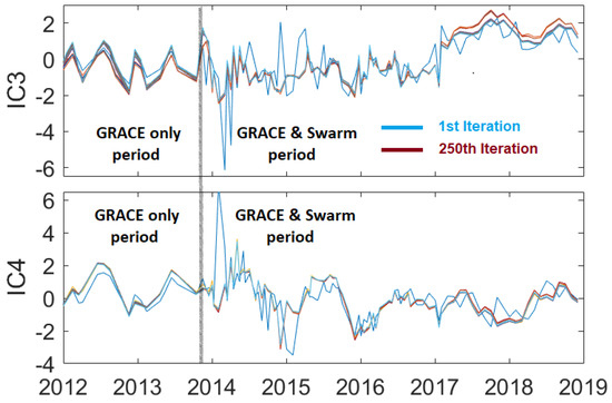
Figure 1.
An overview of changes in empirical independent components (ICs), i.e., third (IC3) and fourth (IC4) independent components, through the iterations of Approach 2. To enhance the visualization, the iteration is limited to 250 and for the period of 2012–2018.
3.4. Estimation of Reconstructions Errors
In order to estimate uncertainties of the reconstruction from Approach 1 and Approach 2, we followed the Bootstrap approach used similar to that in [44]. First, n realizations of the data matrix were generated by considering the original data matrix and adding errors from GRACE and Swarm TWSC fields. The error fields were generated randomly but by considering the TWSC covariances. Applying the three steps of Approach 1 and 2 on these realizations yields n sets of reconstruction results, from which the uncertainty of independent modes was estimated. In the numerical implementation of this study, we selected n to be 1000. These error fields were used to estimated error budget of basin average estimations in Section 4.
4. Results
In this section, first we assessed the reconstruction results from Approach 1 and 2 (Section 4.1) described in the previous section. We show that the iterative reconstruction yields TWSC fields that contain a lower level of noise, and therefore, in Section 4.2, these fields were used to assess water mass changes within the world’s 33 largest river basins. All GRACE fields were smoothed by the Gaussian filter with 500 km half-width radius. Our numerical evaluations indicate that the application of alternative filters such as the DDK anisotropic filters in [37] does not alter the general results of reconstruction, but it might slightly change the basin averaged mass estimations of Section 4.2.
4.1. Evaluating the Reconstruction Results of Approach 1 and 2
First, we compared the results of reconstructions for two arbitrary selected epochs, for which both GRACE and Swarm fields are available. Figure 2A1,B1 indicate GRACE fields in two selected dates in the year 2014 and 2015, where Figure 2A2,B2 show Swarm derived mass estimation for similar dates. By comparing A1 and B1 with A2 and B2, respectively, one can detect similar large-scale mass anomalies, for example over Amazon, Greenland, and North America. The positive–negative anomalies of the northern and southern hemispheres are also well reflected in the Swarm TWSC fields (compare the fields on the first column on left with the second column from left); however, even by a simple visual comparison of the Swarm and GRACE fields, it is clear that mass changes from Swarm data are over-smoothed, i.e., overall a damping of ∼ 1.5 to 2 in terms of standard deviation (StD) was estimated to match Swarm TWSC fields over land to that of GRACE. In general, the anomalies seen over land and the oceans cannot be easily interpreted since they are unrealistically extended over the land area, such as those anomalies over the Australian continent in A2 or those detected over South Asia and Africa in B2, which do not match the results of GRACE in A1 and B1, respectively. This is partly due to the fact that the smoothing radius for denoising GRACE data was 500 km, and 1000 km for Swarm; however, even, GRACE TWSC fields that are smoothed by a filter of 1000 km radius indicate more details than those of Swarm’s (results are not shown here). This happens because the GRACE hl-SST observations are more sensitive to mass redistribution justifying the fact that GRACE data are computed up to higher degree and order potential coefficients (than Swarm).
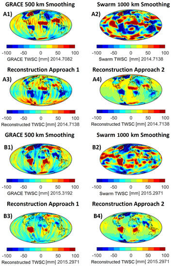
Figure 2.
Results of the two reconstruction techniques for the period that both the Gravity Recovery And Climate Experiment (GRACE) and Swarm fields exist; (A1,B1) show the GRACE fields in 2014.7082 (August 2014) and 2015.3192 (March 2015), respectively, while (A2,B2) indicate Swarm fields close to A1 and B1 (2014.7138 and 2015.2971); (A3,B3) represent the reconstruction results of Approach 1; and finally, (A4,B4) belong to those of Approach 2.
The results of reconstruction from Approach 1 and 2 are shown in Figure 2A3,B3,A4,B4, respectively. These fields can be compared directly to those of GRACE in A1 and B1. In general, we find less magnitude of noise in the TWSC fields of Approach 2 (iterative reconstruction) than those of Approach 1. We show this by computing standard deviation (StD) of differences between the reconstructed values and original GRACE data over land and oceans, where the mean values are reported in Table 1. This was theoretically expected that the iterations in Approach 2 reduces the noise part (any spatially/temporally random behavior) of GRACE and Swarm data. The reason is that the dominant eigenvectors are oriented to retrieve the ‘signal’ part of data and the dominant part of ‘noise’ is discarded (by eigenvalue decomposition and the joint diagonalization of the forth-order cumulants). During the iterations, the orientation of ICs are modified so that their evolution becomes less random. As a result, Approach 2 yields spatially and temporally homogenized reconstruction fields as described in the end of Section 3.3.

Table 1.
Mean of the standard deviation of differences between the reconstructed values and the original GRACE TWSC–terrestrial water storage changes data over the 33 major river basins (marked as land) and rest of the globe (marked as ocean).
Figure 3 contains the TWSC fields of Swarm and the reconstructions that correspond to the middle of 2017 and 2018 (time: 2017.5888, i.e., July 2017, and 2018.4221, i.e., May 2018), where no GRACE data are available. The original Swarm TWSC fields are shown in Figure 3A1,A2, and the reconstruction results of Approach 1 are shown in Figure 3B1,B2. Those of Approach 2 are shown in Figure 3C1,C2. By comparing the extension of anomalies derived from original Swarm data and reconstructions over land, we see that both reconstruction techniques localize the mass anomalies and their patterns are closer to what we expect from GRACE mission. We also notice that the results of Approach 2 better keep the extension of original signal in Swarm. For example, by a visual comparison of Figure 3A1,B1,C1, one can find higher similarity between the dipole anomaly over South America derived from Figure 3A1,C1, compared to that of Figure 3B1, where the extension of anomaly in the northern part of South America is considerably reduced. Another example is the TWSC fields extended over the middle and west parts of Africa, which are detected in Figure 3A1,C1 (amplitude of mm) but the amplitude considerably decreases in Figure 3B1 (amplitude of mm). Considering the selected results in 2018 (Figure 3A2,B2,C2), mass anomalies in the Antarctic are found to be considerably underestimated in the reconstruction results of Approach 1 (an average amplitude of mm from Swarm (Figure 3A2) and Approach 2 (Figure 3C2) versus mm from Approach 1).
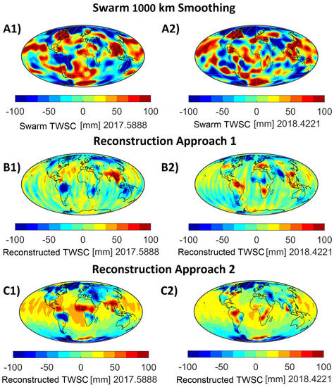
Figure 3.
Results of the two reconstruction techniques for the period that only Swarm fields exist; (A1,A2) show the original Swarm fields in 2017.5888 (July 2017) and 2018.4221 (May 2018), respectively; (B1,B2) indicate the reconstruction results of Approach 1; (C1,C2) represent those of Approach 2.
To make sure that the reconstruction approach works properly, when the GRACE-FO data are available, we extended the time of investigation to end of 2019. Figure 4 compares Swarm (Figure 3A1,A2), the reconstruction of Approach 2 (Figure 3B1,B2), and GRACE-FO (Figure 3C1,C2) that correspond to 2019.2890 (March 2019) and 2019.6246 (July 2019), respectively. Here, we only show the hydrological signals (i.e., oceans ans polar regions are masked). A visual comparison indicates that the reconstructed fields (Figure 3B1,B2) are very close to those of GRACE-FO (in Figure 3C1,C2), compared to those of Swarm (Figure 3A1,A2). An average correlation coefficient of 0.89 are found between the reconstructions and GRACE-FO during 2019.
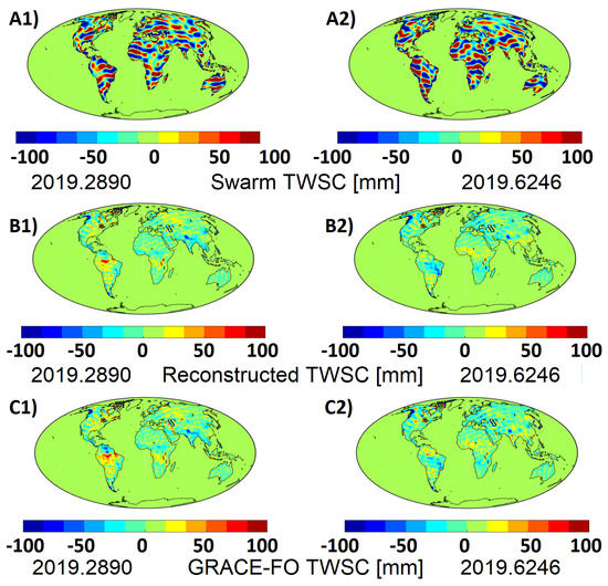
Figure 4.
The reconstruction results of Approach 2 and their comparisons with Swarm and GRACE-FO data; (A1,A2) show the original Swarm fields in 2019.2890 (March 2019) and 2019.6246 (July 2019), respectively; (B1,B2) indicate the reconstruction results of Approach 2; (C1,C2) represent those of GRACE-FO that were not used during the reconstruction. A mask was used to retain the signal over the land.
An evaluation of the noise level and leakage error for smoothed GRACE and Swarm data as well as the reconstructed fields is presented in Appendix B. The results show that the reconstruction considerably improves the accuracy of TWSC estimations, i.e., the level of noise, is reduced by on average and the median of the leakage errors for all the world’s 33 largest river basins is reduced by .
To assess the error behavior of our reconstruction results, Figure 5 shows the differences during 2019.3726 (April 2019) and 2019.7082 (August 2019), where the magnitude of differences over the land area is found to be less than 10 mm (which is acceptable for smoothed TWSC fields). This justifies the suitability of these fields in hydrological studies.
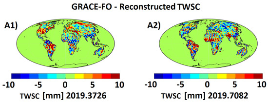
Figure 5.
Differences between GRACE-FO TWSC–terrestrial water storage changes fields and the reconstruction results of Approach 2 in (A1)) 2019.3726 (April 2019) and (A2)) 2019.7082 (August 2019), respectively. A mask is used to retain the signal over the land.
In the light of our results in the previous section, we believe that the reconstruction results from Approach 2 have better quality, i.e., contain less noise and the mass anomalies are well localized. Therefore, these fields are used to assess the global mass redistribution of 2003–2018 in terms of trends, seasonal and sub-seasonal cycles, as well as those related to teleconnection evens, see similar studies, e.g., [14,44,50,56,78]. To illustrate the benefit of the iterations in Approach 2 to reduce the noise in TWSC fields, a comparison between the results of the first iteration with those of 250th iteration in terms of basin-averaged TWSC is shown in Figure A1. An illustration of TWSC time series on two selected regions in the USA (latitude: and longitude: ) and South Africa (latitude: and longitude: ) is shown in Figure A2.
4.2. Mass Changes over 2003–2018 within the World’s 33 Largest River Basins
An overview of mass changes covering 2003–2018 is provided using the reconstructed fields of Approach 2. The fields are averaged within the world’s 33 largest river basins (the same as [79,80]) and compared with 8 lake levels, where the corresponding results are shown in Figure 6, Figure 7, Figure 8, Figure 9, Figure 10, Figure 11, Figure 12 and Figure 13.
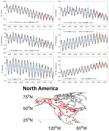
Figure 6.
Basin averages of the reconstructed TWSC estimates within the six major river basins of North America, covering 2003–2018. The red lines show the long-term linear trend and acceleration component fitted to the basin-averaged TWSC estimates using the least squares approach. Note that the values of linear trend (mm/yr) and acceleration (mm/) components fitted to each time series are shown by L-T and Acc, respectively.
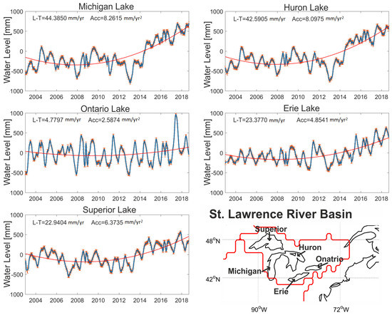
Figure 7.
Satellite altimetry observations within the Great Lakes of Superior, Huron, Michigan, Erie, and Ontario within the St. Lawrence River Basin (North America), covering the period of 2003–2018. The red lines show the long-term linear trend and acceleration component fitted to the water level time series using the least squares approach. The values of linear trend (mm/yr) and acceleration (mm/) components fitted to each time series are shown by L-T and Acc, respectively.
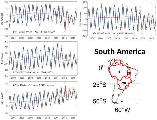
Figure 8.
Basin averages of the reconstructed TWSC fields within the four major river basins of South America covering 2003–2018. The red line shows the long-term linear trend (L-T (mm/yr)) and acceleration (Acc (mm/)) components fitted to the reconstructed TWSC estimates.
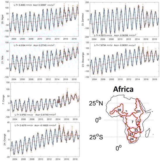
Figure 9.
Basin averages of the reconstructed TWSC fields within the six major river basins of the African continent covering 2003–2018. The red lines show the long-term linear trend (L-T (mm/yr)) and acceleration (Acc (mm/)) components fitted to the TWSC estimates.
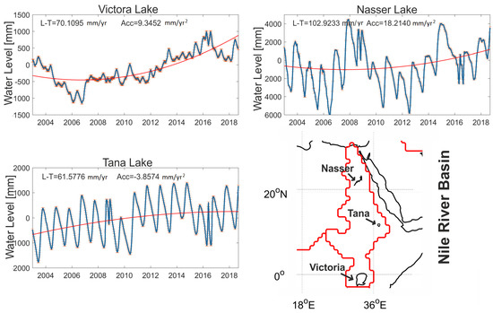
Figure 10.
Satellite altimetry observations within three lakes (Victoria, Nasser, and Tana) within the Nile River Basin (Africa) covering 2003–2018. The red lines show the long-term linear trend (L-T (mm/yr)) and acceleration (Acc (mm/)) components fitted to the altimetry time series.
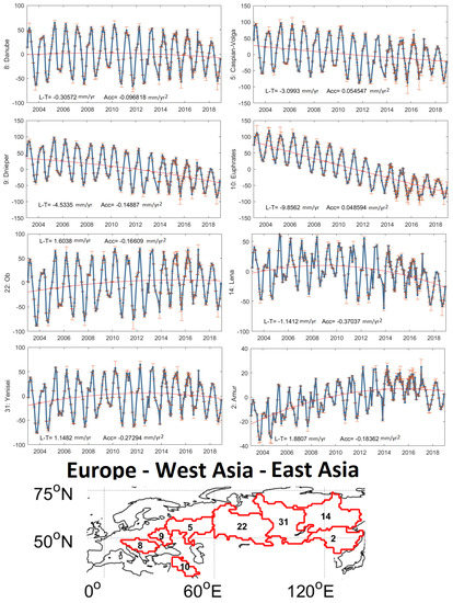
Figure 11.
Basin averages of the reconstructed TWSC fields within the eight major river basins of the Europe and West-East Asia covering 2003–2018. The red lines show the long-term linear trend (L-T) mm/yr)) and acceleration (Acc (mm/)) components fitted to the TWSC estimates.
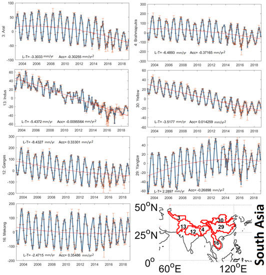
Figure 12.
Basin average of the reconstructed TWSC fields within the seven major river basins of South Asia covering 2003–2018. The red lines show the long-term linear trend (L-T (mm/yr)) and acceleration (Acc (mm/)) components fitted to the TWSC estimates.
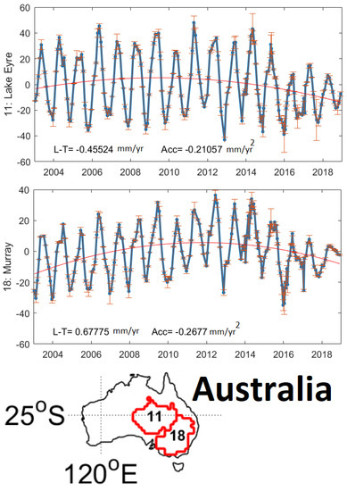
Figure 13.
Basin average of the reconstructed TWSC fields within the two major river basins within the Australian continent covering 2003–2018. The red lines show the long-term linear trend (L-T (mm/yr)) and acceleration (Acc (mm/)) components fitted to the TWSC estimates.
Linear trend, acceleration corresponding to inter-annual or longer climate episodes (with respect to the time 2010.5) along with annual and semi-annual cycles were extracted from basin-averaged TWSC time series within the 33 basins using a linear model (, where contains the basin averaged TWSC; t is the time in year minus 2010.5; are coefficients to be estimated using a least squares fit; contains the residuals). The significance of these coefficients, e.g., a for the linear trend and b for non-linear trend (or known as acceleration) was evaluated using a Fisher test as in [6], and the results are summarized in Table 2. In the following, we report some features of the basin averaged TWSC that are relevant to make sure the reconstructed TWSC fields are reliable to be used for large-scale hydrological assessments. The results are reported according to different continents.
Table 2.
The amplitude of linear trend [mm/yr] and acceleration [mm/] fitted to the basin averaged reconstructed global terrestrial water storage change (TWSC) fields within the world’s 33 major river basins covering 2003–2019. Statistically significant trends and accelerations are distinguished by bold text. Note that only the first two digits after the decimal point are significant.
North America: Six river basins are shown in Figure 6, for which statistically significant linear trends are found within the Yukon, Mackenzie, Mississippi, and St. Lawrence River Basins. The non-linear trend (simply called acceleration in what follows) component is not found to be statistically significant in any of the six basins in North America. Positive linear trend is found in the St. Lawrence and Mississippi River Basins that are consistent with independent measurements. Here, we considered altimetry measurements (from https://ipad.fas.usda.gov/cropexplorer/global_reservoir/) to test whether surface water storage (as suggested by [81]) is a dominant contributor to TWSC trends within the St. Lawrence River Basin containing the Great Lakes of Superior, Huron, Michigan, Erie, and Ontario. Our results indicate that the level of these five lakes increased during 2003–2018 as shown in Figure 7. It seems that the increase in surface water causes the positive trends derived from our reconstructed fields. It is worth mentioning here that the use of altimetry data in this study was to provide an evidence of changes in trends and seasonality rather than providing a quantitative assessment of these components, because for the latter, one needs to implement a sophisticated leakage reduction (e.g., [54]), which will be performed in future.
Linear trends in four other river basins, Yukon, Nelson, Mackenzie, and Colorado are found to be negative, which can be associated to both irrigation and global warming. For example, Lena and Mackenzie are two glacier-dominant basins in the Arctic region influenced by the climate warming over the past four decades, and consequently, caused decreasing in water storage in these regions [82,83,84]. Scanlon et al. [85] indicated that Colorado River Basin experienced multiyear intense droughts between 1980 to 2015, and storage depletion in this basin is dominated by reductions in surface reservoir and soil moisture storage, as well as reductions in groundwater storage due to imbalances between water supplies and demands during the climate extremes.
South America: Four basins are assessed in South America, with no significant trends in the three basins of Amazon, Orinoco, and Tocantins (except Parana). The magnitude of seasonal TWSC considerably decreased in all the basins, which can be attributed to the drought events, for which, e.g., [86,87] indicated that tropical and sub-tropical South America has experienced several extreme hydrological droughts in the last decades, e.g., 2005, 2010, and 2016 droughts, due to higher than usual sea surface temperatures in the Tropical Pacific (including El Niño events) and Atlantic Oscillations; however, the hydrological consequences due to the drought of 2016 are reported to be more severe than previous ones (see e.g., [86,88,89]).
The increasing linear trend in water storage within the Parana River Basin, despite of no significant rainfall increases, can be explained by increasing the mean annual discharge during the last 2 decades by converting forests to agricultural land (see, e.g., [90,91]). The small decrease in the magnitude of seasonal TWSC within the Parana River Basin during 2017–2018 can be attributed to the extreme drought of 2016 (see the trend values in Table 2).
Africa: Six river basins are assessed in the African continent (see Figure 9). The linear trends in the Niger, Nile, Okavango, and Orange River Basins, and the acceleration in Congo are found to be statistically significant. Figure 10 shows that the level of three major lakes within the Nile River Basin from altimetry measurements. For all three lakes, a positive trend is found during the period of 2003–2018, which is correlated with our finding from the reconstructed TWSC fields within this basin.
The Niger River Basin is the third longest river in Africa and located across several east–west oriented climate zones, which causes a complex composition of geographical factors. These factors, as well as the impact of climate changes [92,93] can be the reason of intense pressure on water resources in this region [94]. Many studies such as [95,96,97] indicated that because of the changes in land cover and the expansion of agriculture in Nigerian Sahel, discharge regime has been changes and as a result the groundwater storage increased in this basin, which is reflected in the reconstructed TWSC estimates.
The positive trends in TWSCs of Okavango can be associated to the heavy rainfalls, seasonal floods, and geographical location of Okavango Delta, which cause the flow of water into this Delta. The time period of the seasonal floods in Okavango Delta are varied in different years; however, it generally occurs between March and May every year just after the local summer rains (between November and March) in the region of the Delta [98,99]. Although the positive linear trends in TWSC is found in Africa, decreasing in the magnitude of seasonal TWSC in 2017–2018 is caused by the low net-fluxes after the extreme drought of 2015/2016 (see, e.g., [87]). This should be noted here that a separate interpretation of changes in precipitation or evaporation on TWSC should be performed with care. For example, [100] indicate how changes in moisture transport impact hydrological cycle changes. As a result, not necessarily, an increase or decrease of fluxes would change the seasonal amplitude of the TWSC in the same direction.
Europe, West Asia, and East Asia: Among eight major river basins of the Europe and West and East Asia, statistically significant linear TWSC trends can only be observed within the Euphrates (with negative trend) and Amur (with positive trend) River Basins. Voss et al. [101] and Forootan et al. [6] reported a significant decline in groundwater, soil moisture, and surface water storage within the Euphrates River Basin between 2003–2013, which was associated to both irrigation and long-term net-precipitation deficit. Increasing trend in TWSC of Amur River Basin can be due to the increases in deforestation of coniferous forests, which contributed to the increases in rivers’ flow and flood events in this basin (see, e.g., [102]). A negative linear trend can be seen in reconstructed TWSCs within the Lena River Basin, which is intensified during 2014–2018. Previous studies, e.g., [84,103], argue that warmer temperatures due to climate change have impacted the hydrological regime of rivers within this basin via changes in precipitation type (rain replacing snow). They also hypothesize that other factors, such as the melting of permafrost, glaciers, and/or changes in groundwater conditions to have contributed to this trend; therefore, our results confirm their independent investigations. It also provides an evidence of the contribution of water storage decline in the detected change in hydrological regime.
Figure 11 indicates that the reconstructed TWSCs within the Ob and Yenisei River Basins do not contain considerable linear trends, and small trend values are detected within Dnieper, Danube, and Caspian-Volga as part of the European Russia. Grigoriev et al. [104] analysed TWSC in the European part of Russia and found a non-significant reduction in the TWSC between 2002–2015, which was caused by a decline in surface and groundwater water storage.
South Asia: Seven basins are assessed in the South Asia, where all except the Yangtze River Basin experienced a long-term decrease in TWSC during 2003–2018. Largest decreasing trends are found in basins with large scale irrigation such as Ganges, Indus, Barhmaputra, and Yellow River Basins that are strongly affected by climate change. These results confirm the findings by [87,105,106,107].
A negative linear trend is detected in TWSC of the Aral and Mekong River Basins. In recent decades, irrigation is highly developed in both of these basins [108,109]. Analysis of the water flow development in Aral Basin indicated that the water diversion and irrigation schemes in this region have considerably increased evapo-transpiration and consequently, decreased net water flux from the atmosphere to the surface of the Aral Basin [110]. These factors cause a reduction in the magnitude of seasonal amplitude of TWSCs within both of these basins.
Sun et al. [111] used GRACE data, flood potential index, as well as precipitation and other meteorological data to generate monthly terrestrial water storage anomalies and evaluated the flood potential in the Yangtze River Basin. Their results indicated that the amounts of water storage increased from 2003 to 2014, which confirms the increasing linear trend in the reconstructed TWSC of this study (numerical values of trends and accelerations are reported in Table 2).
Australian: The two major basins of Murray and Lake Eyre are assessed here with no significant linear trend; however, the acceleration component is found to be negative for both basins. Lakshmi et al. [112] analyzed the variability of individual water balance components in the major river basins of the world between 2002 and 2015. They showed that the maximum precipitation anomaly, as well as runoff and soil moisture anomaly within the Murray River Basin happened during 2011. Their result agree with the small positive trend and negative acceleration component of reconstructed TWSC within the Murray River Basin. Figure 13 shows that the the peak of TWS changes in Murray River Basin was happened in 2012. The associated time lag between maximum precipitation anomaly in 2011 (shows by [112]), and the maximum TWS changes in 2012 could be influenced by different factors such as climatic conditions, vegetation density, runoff path-length, different recharge characteristics, permeability of sediments, and the abundance of surface water bodies (see e.g., [113,114,115]). Forootan et al. [116] argued that the increasing rainfall trends over the last 30 years, such as heavy rainfall in 2010 and 2011 over Murray and Lake Eyre River Basins, were mainly due to La Niña events. A decrease in 2012–2018 TWSC caused a negative acceleration in the reconstructed TWSC estimates of these two basins, which can be a response to the Millennium meteorological drought of 2000–2009 (see, e.g., [117] and www.water.vic.gov.au/climate-change/millennium-drought-report).
5. Summary and Conclusions
In this study, two statistical reconstruction formulations (Approach 1 and Approach 2) are provided, which can be used to merge time-variable satellite gravity solutions with distinct accuracy and signal spectral contents. Here, these approaches are implemented to merge the total water storage change (TWSC) products of two mission GRACE (2003–2017) and the three-satellite constellation Swarm (2013–now). This integration bridges the one year gap between GRACE and GRACE Follow-On mission, providing a consistent fields covering 2003–2018.
The formulation of Approach 1 follows a common data reconstruction procedure similar to [27], and Approach 2 is an iterative reconstruction using the whole period of available GRACE and Swarm data. For both formulations, we applied independent component analysis (ICA, [13,43]) to reduce the noise in original fields. We tested these techniques numerically in various ways, i.e., in terms of global empirical base functions (shown in Figure 1), in the global grid domain (Figure 2 and Figure 3), and finally in terms of basin averages (Section 4.2).
All investigations show that both of the reconstruction techniques decrease the noise level in Swarm gravity fields and improve their spatial resolution. The results of Approach 2 provide more homogenized (long-term) TWSC fields, which are recommended for studies addressing global mass redistribution. Otherwise, the considerably high level of noise in Swarm data and their inconsistencies with GRACE(-FO) does not allows their applications to study long term hydrological changes in river basins (see e.g., Figure A1). Comparisons of the reconstruction results (Approach 2) with those of GRACE-FO in 2019 show that the magnitude of differences is smaller than 10 mm; therefore, these TWSC fields are used to monitor hydrological changes of the world’s 33 largest river basins covering 2003–2018, where we find:
- positive linear temporary trends in the St. Lawrence and Mississippi River Basins, caused by changes in surface water compartment and confirmed by altimetry measurements as an independent comparison;
- negative linear temporary trends in TWSC of the Yukon, Nelson, Mackenzie, and Colorado River Basin, which can be associated to both irrigation and global warming;
- a considerable decrease in the magnitude of the seasonal cycle within the four investigated basins in South America (Amazon, Orinoco, Tocantins, and Parana) that is attributed to the drought events of 2016–2018;
- a mixed positive and negative temporary trends in the basins within Africa, where that of Nile was dominated by the surface water in lakes such as Victoria, but that of Niger was associated to groundwater; and those of Congo, Okavango, Orange, and Zambezi were influenced by an increase in the rainfall;
- the impact of anthropogenic impacts on Euphrates, Ganges, Indus, and Brahmaputra, Murray (negative trend) as well as Amur (positive trend).
The values of these inter-annual climate episode driven trends in the TWSCs are reported in Table 2. The proposed reconstruction methodology can potentially replace the contemporary techniques trying to optimally derive the relative data weights between two different data types. The reconstructed fields of Approach 2, which was used to estimate basin averages within the world’s 33 largest river basin, will be provided upon request. A global monthly reconstruction of TWSC fields is provided as supplementary material of this paper. These fields are generated on 1 degree global grids with the Gaussian smoothing of 500 km (half-radius) using the iterative ICA reconstruction and cover the period of 2002–2020.
Supplementary Materials
The following are available online at https://www.mdpi.com/2072-4292/12/10/1639/s1, Reconstructed monthly TWSC fields of 2002-2020-1 deg resolution filtered by Gaussian 500 km half-radius.
Author Contributions
Conceptualization, E.F. and C.K.S.; methodology, E.F. and M.J.T.; software, E.F., M.S., and N.M.; validation, E.F., N.M., S.F. and A.B.; formal analysis, A.B., M.S., S.F., C.Z., and Y.Z.; investigation, E.F., M.S., N.M., S.F., and C.K.S.; resources, E.F. and C.K.S.; data curation, A.B., C.Z., and Y.Z.; writing—original draft preparation, E.F., M.S., and N.M.; writing—review and editing, C.K.S., A.B., and M.J.T.; visualization, E.F. and N.M.; supervision, E.F.; project administration, E.F.; funding acquisition, E.F. All authors have read and agreed to the published version of the manuscript.
Funding
This research received no external funding.
Acknowledgments
The authors are grateful to the comments provided by the Associate Editor and four anonymous reviewers, which are used to improve the quality of this work. We acknowledge data product providers of GRACE, Swarm and altimetry products used in this study. E. Forootan thanks DAAD for the fund 57445178. N. Mehrnegar is grateful to the Cardiff University’s Vice Chancellor fund, which supports her PhD research. C.K. Shum, Yu Zhang, and Chaoyang Zhang are partially supported by ESA’s Swarm DISC Project (SW-CO-DTU-GS-111), Strategic Priority Research Program of the Chinese Academy of Sciences (XDA19070302), and National Key Research & Development Program of China (017YFA0603103). A. Bezděk is supported by the project LTT18011.
Conflicts of Interest
The authors declare no conflict of interest.
Appendix A. Impact of Iterations in Approach 2 on Independent Components
A comparison between TWSC estimations derived from the iteration 1 and 250 of Approach 2 was performed. The basin averaged results are shown in Figure A1 for three arbitrary selected river basins of Indus, Mackenzie, and Orinoco. It is clear from the graphs that the noise in Swarm data disturb estimation of trend, acceleration, and even interpretation of the seasonal scale changes in TWS; therefore, Swarm TWSC fields without implementing a reasonable post-processing cannot be used along-side GRACE data to assess hydrological changes within river basins. The noise has however almost vanished in the 250th iteration, where the red curves indicate smooth evolution of TWSC in the river basins as interpreted in Figure 6, Figure 7, Figure 8, Figure 9, Figure 10, Figure 11, Figure 12 and Figure 13.

Figure A1.
A comparison between basin averaged TWSC estimations derived from the iteration 1 and 250 of the reconstruction-Approach 2. The results are shown for three arbitrary selected river basins.
Figure A1.
A comparison between basin averaged TWSC estimations derived from the iteration 1 and 250 of the reconstruction-Approach 2. The results are shown for three arbitrary selected river basins.

In order to illustrate the impact of the iterative reconstruction on the TWSC estimations, here we select two arbitrary points in the USA (latitude: and longitude: ) and South Africa (latitude: and longitude: ). The time series of TWSC from the reconstruction were compared with those of GRACE, GRACE-FO, Swarm. The results in Figure A2 show that the reconstruction, not only fills the gap between GRACE and GRACE-FO, it also homogenizes the temporal evolution of TWSC. This is clear by comparing the original TWSC from Swarm (marked by stars) with those of reconstruction (marked by empty circles). Here, the gap periods are highlighted by colored boxes.

Figure A2.
A comparison of TWSC estimations for two arbitrary points in the USA (top) and South Africa (bottom).
Figure A2.
A comparison of TWSC estimations for two arbitrary points in the USA (top) and South Africa (bottom).

Appendix B. Noise and Leakage Estimation of the Reconstructed TWSC Fields
In this Appendix, we first assessed the level of noise in the original TWSC (i.e., smooth GRACE and Swarm TWSC) and reconstructed fields (compare Figure A3 top with bottom). For this estimation, the noise level is considered to be corresponded with of the less dominant eigenvalues as discussed in Approach 1 and 2. The results indicate that the noise pattern of > 10 mm (which is a common noise level expectation from smoothed GRACE TWSC fields) in terms of TWSC vanishes in the reconstruction fields to < 3 mm.
In Figure A4, an estimation of the spatial leakage error (computed following [38]) is shown for three river basins of different size, i.e., Amazon as the largest river basin, and the area of Amur and Aral is relatively smaller. Numerical results indicate that the leakage error during the Swarm era (2013–2018) has been considerably decreased. The error in Amazon is decreased from an average of ∼ 3 mm to less than ∼ 1 mm, while in Amur this is found to be decreased from ∼ 9 mm on average to ∼ 4 mm, and finally in Aral, from ∼ 19 mm to ∼ 7 mm.

Figure A3.
A comparison between the noise level of TWSC fields before (A: left) and after reconstruction (B: right).
Figure A3.
A comparison between the noise level of TWSC fields before (A: left) and after reconstruction (B: right).

An overall overview of the enhancement in the estimation of basin-averaged spatial leakage is shown in Figure A5, where the estimations correspond to the original GRACE (covering 2003–2014) and Swarm data (2013–2018). We also show the estimated standard deviation of leakage errors for the same periods but from the reconstructed results (Approach 2). Our numerical investigations indicate that the standard deviation (StD) of leakage errors that correspond to the Swarm data (with an average of ∼ 15 mm) is ∼ three times bigger than that of GRACE (with an average of ∼ 5 mm covering 2003–2014). After the reconstruction, very comparable level of leakage errors is derived over the GRACE and Swarm era (i.e., on average ∼ 3.5 mm).

Figure A4.
Estimated leakage error for the tree river basins of Amazon (top), Amur (middle), and Aral (bottom) river Basins.
Figure A4.
Estimated leakage error for the tree river basins of Amazon (top), Amur (middle), and Aral (bottom) river Basins.


Figure A5.
An overview of the standard deviation of the estimated leakage error for the world’s 33 river basins.
Figure A5.
An overview of the standard deviation of the estimated leakage error for the world’s 33 river basins.

References
- Tapley, B.D.; Bettadpur, S.; Ries, J.C.; Thompson, P.F.; Watkins, M.M. GRACE measurements of mass variability in the Earth system. Science 2004, 305, 503–505. [Google Scholar] [CrossRef] [PubMed]
- Elsaka, B.; Forootan, E.; Alothman, A. Improving the recovery of monthly regional water storage using one year simulated observations of two pairs of GRACE-type satellite gravimetry constellation. J. Appl. Geophys. 2014, 109, 195–209. [Google Scholar] [CrossRef]
- Flechtner, F. GFZ Level-2 Processing Standards Document for Level-2 Product Release 0004. 2007. Available online: http://icgem.gfz-potsdam.de/L2-GFZ_ProcStds_0005_v1.1-1.pdf (accessed on 20 May 2020).
- Shum, C.K.; Guo, J.Y.; Hossain, F.; Duan, J.; Alsdorf, D.E.; Duan, X.J.; Kuo, C.Y.; Lee, H.; Schmidt, M.; Wang, L. Inter-annual water storage changes in Asia from GRACE data. In Climate Change and Food Security in South Asia; Springer: Amsterdam, The Netherlands, 2010; pp. 69–83. [Google Scholar] [CrossRef]
- Forootan, E.; Rietbroek, R.; Kusche, J.; Sharifi, M.A.; Awange, J.L.; Schmidt, M.; Omondi, P.; Famiglietti, J.S. Separation of large scale water storage patterns over Iran using GRACE, altimetry and hydrological data. Remote. Sens. Environ. 2014, 140, 580–595. [Google Scholar] [CrossRef]
- Forootan, E.; Safari, A.; Mostafaie, A.; Schumacher, M.; Delavar, M.; Awange, J.L. Large-scale total water storage and water flux changes over the arid and semiarid parts of the Middle East from GRACE and reanalysis products. Surv. Geophys. 2017, 38, 591–615. [Google Scholar] [CrossRef]
- Awange, J.L.; Forootan, E.; Kuhn, M.; Kusche, J.; Heck, B. Water storage changes and climate variability within the Nile Basin between 2002 and 2011. Adv. Water Resour. 2014, 73, 1–15. [Google Scholar] [CrossRef]
- Ahmed, M.; Sultan, M.; Wahr, J.; Yan, E. The use of GRACE data to monitor natural and anthropogenic induced variations in water availability across Africa. Earth Sci. Rev. 2014, 136, 289–300. [Google Scholar] [CrossRef]
- Forootan, E.; Awange, J.L.; Kusche, J.; Heck, B.; Eicker, A. Independent patterns of water mass anomalies over Australia from satellite data and models. Remote. Sens. Environ. 2012, 124, 427–443. [Google Scholar] [CrossRef]
- Andrew, R.L.; Guan, H.; Batelaan, O. Large-scale vegetation responses to terrestrial moisture storage changes. Hydrol. Earth Syst. Sci. 2017, 21, 4469–4478. [Google Scholar] [CrossRef]
- Tangdamrongsub, N.; Han, S.C.; Tian, S.; Müller Schmied, H.; Sutanudjaja, E.H.; Ran, J.; Feng, W. Evaluation of groundwater storage variations estimated from GRACE data assimilation and state-of-the-art land surface models in Australia and the North China Plain. Remote. Sens. 2018, 10, 483. [Google Scholar] [CrossRef]
- Syed, T.H.; Famiglietti, J.S.; Rodell, M.; Chen, J.; Wilson, C.R. Analysis of terrestrial water storage changes from GRACE and GLDAS. Water Resour. Res. 2008, 44, W02433. [Google Scholar] [CrossRef]
- Forootan, E.; Kusche, J. Separation of global time-variable gravity signals into maximally independent components. J. Geod. 2012, 86, 477–497. [Google Scholar] [CrossRef]
- Kusche, J.; Eicker, A.; Forootan, E.; Springer, A.; Longuevergne, L. Mapping probabilities of extreme continental water storage changes from space gravimetry. Geophys. Res. Lett. 2016, 43, 8026–8034. [Google Scholar] [CrossRef]
- Long, D.; Pan, Y.; Zhou, J.; Chen, Y.; Hou, X.; Hong, Y.; Scanlon, B.R.; Longuevergne, L. Global analysis of spatiotemporal variability in merged total water storage changes using multiple GRACE products and global hydrological models. Remote. Sens. Environ. 2017, 192, 198–216. [Google Scholar] [CrossRef]
- Scanlon, B.R.; Zhang, Z.; Save, H.; Sun, A.Y.; Schmied, H.M.; Van Beek, L.P.; Wiese, D.N.; Wada, Y.; Long, D.; Reedy, R.C.; et al. Global models underestimate large decadal declining and rising water storage trends relative to GRACE satellite data. Proc. Natl. Acad. Sci. USA 2018, 115, E1080–E1089. [Google Scholar] [CrossRef]
- Tapley, B.D.; Watkins, M.M.; Flechtner, F.; Reigber, C.; Bettadpur, S.; Rodell, M.; Sasgen, I.; Famiglietti, J.S.; Landerer, F.W.; Chambers, D.P.; et al. Contributions of GRACE to understanding climate change. Nat. Clim. Chang. 2019, 9, 358–369. [Google Scholar] [CrossRef]
- Flechtner, F.; Neumayer, K.H.; Dahle, C.; Dobslaw, H.; Fagiolini, E.; Raimondo, J.C.; Güntner, A. What can be expected from the GRACE-FO laser ranging interferometer for Earth science applications? Surv. Geophys. 2016, 33, 453–470. [Google Scholar] [CrossRef]
- Rietbroek, R.; Fritsche, M.; Dahle, C.; Brunnabend, S.E.; Behnisch, M.; Kusche, J.; Flechtner, F.; Schröter, J.; Dietrich, R. Can GPS-derived surface loading bridge a GRACE mission gap? Surv. Geophys. 2014, 35, 1267–1283. [Google Scholar] [CrossRef]
- Cecilia Peralta, F.; James H., M.; Wallace, J.M. Proxy representation of Arctic ocean bottom pressure variability: Bridging gaps in GRACE observations. Geophys. Res. Lett. 2016, 43, 9183–9199. [Google Scholar] [CrossRef]
- Lück, C.; Kusche, J.; Rietbroek, R.; Löcher, A. Time-variable gravity fields and ocean mass change from 37 months of kinematic Swarm orbits. Solid Earth 2018, 9, 323–339. [Google Scholar] [CrossRef]
- Cheng, M.K.; Shum, C.K.; Tapley, B.D. Determination of long-term changes in the Earth’s gravity field from satellite laser ranging observations. J. Geophys. Res. Solid Earth 1997, 102, 22377–22390. [Google Scholar] [CrossRef]
- Cheng, M.; Tapley, B.D. Seasonal variations in low degree zonal harmonics of the Earth’s gravity field from satellite laser ranging observations. J. Geophys. Res. Solid Earth 1999, 104, 2667–2681. [Google Scholar] [CrossRef]
- Cox, C.M.; Chao, B.F. Detection of a large-scale mass redistribution in the terrestrial system since 1998. Science 2002, 297, 831–833. [Google Scholar] [CrossRef] [PubMed]
- Cheng, M.; Tapley, B.D. Variations in the Earth’s oblateness during the past 28 years. J. Geophys. Res. Solid Earth 2004, 109. [Google Scholar] [CrossRef]
- Sośnica, K.; Jäggi, A.; Meyer, U.; Thaller, D.; Beutler, G.; Arnold, D.; Dach, R. Time variable Earth’s gravity field from SLR satellites. J. Geod. 2015, 89, 945–960. [Google Scholar] [CrossRef]
- Talpe, M.J.; Nerem, R.S.; Forootan, E.; Schmidt, M.; Lemoine, F.G.; Enderlin, E.M.; Landerer, F.W. Ice mass change in Greenland and Antarctica between 1993 and 2013 from satellite gravity measurements. J. Geod. 2017, 91, 1283–1298. [Google Scholar] [CrossRef]
- Haberkorn, C.; Bloßfeld, M.; Bouman, J.; Fuchs, M.; Schmidt, M. Towards a consistent estimation of the earth’s gravity field by combining normal equation matrices from GRACE and SLR. In IAG 150 Years; Springer: Berlin, Germany, 2015; pp. 375–381. [Google Scholar] [CrossRef]
- Friis Christensen, E.; Lühr, H.; Knudsen, D.; Haagmans, R. Swarm–an Earth observation mission investigating geospace. Adv. Space Res. 2008, 41, 210–216. [Google Scholar] [CrossRef]
- Jäggi, A.; Dahle, C.; Arnold, D.; Bock, H.; Meyer, U.; Beutler, G.; Van den IJssel, J. Swarm kinematic orbits and gravity fields from 18 months of GPS data. Adv. Space Res. 2016, 57, 218–233. [Google Scholar] [CrossRef]
- Bezděk, A.; Sebera, J.; Teixeira da Encarnação, J.; Klokočník, J. Time-variable gravity fields derived from GPS tracking of Swarm. Geophys. J. Int. 2016, 205, 1665–1669. [Google Scholar] [CrossRef]
- Meyer, U.; Sosnica, K.; Arnold, D.; Dahle, C.; Thaller, D.; Dach, R.; Jäggi, A. SLR, GRACE and SWARM gravity field determination and combination. Remote. Sens. 2019, 11, 956. [Google Scholar] [CrossRef]
- Dahle, C.; Flechtner, F.; Murböck, M.; Michalak, G.; Neumayer, K.; Abrykosov, O.; Reinhold, A.; König, R. GRACE 327-743 (Gravity Recovery and Climate Experiment): GFZ Level-2 Processing Standards Document for Level-2 Product Release 06 (Rev. 1.0, October 26, 2018); Scientific Technical Report STR—Data; 18/04; GFZ German Research Centre for Geosciences: Potsdam, Germany, 2018; p. 20. [Google Scholar] [CrossRef]
- Jekeli, C. Alternative Methods to Smooth the Earth’s Gravity Field; Reports of the Department of Geodetic Science; 327; The Ohio State University: Columbus, OH, USA, 1981. [Google Scholar]
- Swenson, S.; Wahr, J. Post-processing removal of correlated errors in GRACE data. Geophys. Res. Lett. 2006, 33. [Google Scholar] [CrossRef]
- Kusche, J. Approximate decorrelation and non-isotropic smoothing of time-variable GRACE-type gravity field models. J. Geod. 2007, 81, 733–749. [Google Scholar] [CrossRef]
- Kusche, J.; Schmidt, R.; Petrovic, S.; Rietbroek, R. Decorrelated GRACE time-variable gravity solutions by GFZ, and their validation using a hydrological model. J. Geod. 2009, 83, 903–913. [Google Scholar] [CrossRef]
- Khaki, M.; Forootan, E.; Kuhn, M.; Awange, J.L.; Longuevergne, L.; Wada, Y. Efficient basin scale filtering of GRACE satellite products. Remote. Sens. Environ. 2018, 204, 76–93. [Google Scholar] [CrossRef]
- Da Encarnação, J.T.; Arnold, D.; Bezděk, A.; Dahle, C.; Doornbos, E.; Van den IJssel, J.; Jäggi, A.; Mayer-Gürr, T.; Sebera, J.; Visser, P.; et al. Gravity field models derived from Swarm GPS data. Earth Planets Space 2016, 68, 127. [Google Scholar] [CrossRef]
- Longuevergne, L.; Wilson, C.; Scanlon, B.; Cretaux, J. GRACE water storage estimates for the Middle East and other regions with significant reservoir and lake storage. Hydrol. Earth Syst. Sci. Discuss. 2013, 17, 4817–4830. [Google Scholar] [CrossRef]
- Li, F.; Kusche, J.; Rietbroek, R.; Wang, Z.; Forootan, E.; Schulze, K.; Lück, C. Comparison of data-driven techniques to reconstruct (1992–2002) and predict (2017–2018) GRACE-like gridded total water storage changes using climate inputs. Water Resour. Res. 2020, 56, e2019WR026551. [Google Scholar] [CrossRef]
- Preisendorfer, R.W.; Mobley, C.D.; Barnett, T.P. The principal discriminant method of prediction: Theory and evaluation. J. Geophys. Res. Atmos. 1988, 931, 10815–10830. [Google Scholar] [CrossRef]
- Forootan, E.; Kusche, J. Separation of deterministic signals using Independent Component Analysis (ICA). Stud. Geophys. Geod. 2013, 57, 17–26. [Google Scholar] [CrossRef]
- Forootan, E.; Kusche, J.; Talpe, M.; Shum, C.K.; Schmidt, M. Developing a Complex Independent Component Analysis (CICA) technique to extract non-stationary patterns from geophysical time series. Surv. Geophys. 2018, 39, 435–465. [Google Scholar] [CrossRef]
- Frappart, F.; Ramillien, G.; Maisongrande, P.; Bonnet, M.P. Denoising satellite gravity signals by independent component analysis. IEEE Geosci. Remote. Sens. Lett. 2011, 7, 421–425. [Google Scholar] [CrossRef]
- Frappart, F.; Ramillien, G.; Leblanc, M.; Tweed, S.O.; Bonnet, M.P.; Maisongrande, P. An independent component analysis filtering approach for estimating continental hydrology in the GRACE gravity data. Remote. Sens. Environ. 2011, 115, 187–204. [Google Scholar] [CrossRef]
- Forootan, E. Statistical Signal Decomposition Ttechniques for Analyzing Time-Variable Satellite Gravimetry Data. Ph.D. Thesis, University of Bonn, Bonn, Germany, 2014. [Google Scholar]
- Church, J.A.; White, N.J.; Coleman, R.; Lambeck, K.; Mitrovica, J.X. Estimates of the regional distribution of sea level rise over the 1950–2000 period. J. Clim. 2004, 17, 2609–2625. [Google Scholar] [CrossRef]
- Güntner, A.; Stuck, J.; Werth, S.; Döll, P.; Verzano, K.; Merz, B. A global analysis of temporal and spatial variations in continental water storage. Water Resour. Res. 2007, 43, W05416. [Google Scholar] [CrossRef]
- Mehrnegar, N.; Jones, O.; Singer, M.B.; Schumacher, M.; Bates, P.; Forootan, E. Comparing global hydrological models and combining them with GRACE by dynamic model data averaging (DMDA). Adv. Water Resour. 2020, 138, 103528. [Google Scholar] [CrossRef]
- Chambers, D.P.; Willis, J.K. A global evaluation of ocean bottom pressure from GRACE, OMCT, and steric-corrected altimetry. J. Atmos. Ocean. Technol. 2010, 27, 1395–1402. [Google Scholar] [CrossRef]
- Macrander, A.; Boening, C.; Boebel, O.; Schroeter, J. Validation of GRACE Gravity Fields by In-Situ Data of Ocean Bottom Pressure. In System Earth via Geodetic-Geophysical Space Techniques. Advanced Technologies in Earth Sciences (2190-1643); Flechtner, F., Ed.; Springer: Berlin/Heidelberg, Germany, 2010. [Google Scholar] [CrossRef]
- Chen, Q.; Poropat, L.; Zhang, L.; Dobslaw, H.; Weigelt, M.; Van Dam, T. Validation of the EGSIEM GRACE gravity fields using GNSS coordinate timeseries and in-situ ocean bottom pressure records. Remote Sens. 2018, 10, 1976. [Google Scholar] [CrossRef]
- Moore, P.; Williams, S.D.P. Integration of altimetric lake levels and GRACE gravimetry over Africa: Inferences for terrestrial water storage change 2003–2011. Water Resour. Res. 2014, 50, 9696–9720. [Google Scholar] [CrossRef]
- Awange, J.L.; Forootan, E.; Fleming, K.; Odhiambo, G. Dominant patterns of water storage changes in the Nile Basin during 2003–2013. Remote. Sens. Terr. Water Cycle 2014, 206, 367. [Google Scholar] [CrossRef]
- Eicker, A.; Forootan, E.; Springer, A.; Longuevergne, L.; Kusche, J. Does GRACE see the terrestrial water cycle “intensifying”? J. Geophys. Res. Atmos. 2016, 121, 733–745. [Google Scholar] [CrossRef]
- Bettadpur, S. Gravity Recovery and Climate Experiment Level-2 Gravity Field Product User Handbook. Center for Space Research at The University of Texas at Austin, 2018. Available online: https://podaac-tools.jpl.nasa.gov/drive/files/allData/grace/docs/L2-UserHandbook_v4.0.pdf (accessed on 20 May 2020).
- Visser, P.; Doornbos, E.; Van den IJssel, J.; Da Encarnação, J.T. Thermospheric density and wind retrieval from Swarm observations. Earth Planets Space 2013, 65, 12. [Google Scholar] [CrossRef]
- Olsen, N.; Friis-Christensen, E.; Floberghagen, R.; Alken, P.; Beggan, C.D.; Chulliat, A.; Doornbos, E.; Da Encarnação, J.T.; Hamilton, B.; Hulot, G.; et al. The Swarm satellite constellation application and research facility (SCARF) and Swarm data products. Earth Planets Space 2013, 65, 1189–1200. [Google Scholar] [CrossRef]
- Zehentner, N.; Mayer-Gürr, T. Precise orbit determination based on raw GPS measurements. J. Geod. 2016, 90, 275–286. [Google Scholar] [CrossRef]
- Guo, J.; Shang, K.; Jekeli, C.; Shum, C. On the energy integral formulation of gravitational potential differences from satellite-to-satellite tracking. Celest. Mech. Dyn. Astron. 2015, 121, 415–429. [Google Scholar] [CrossRef]
- Bezděk, A.; Sebera, J.; Klokočník, J.; Kosteleckỳ, J. Gravity field models from kinematic orbits of CHAMP, GRACE and GOCE satellites. Adv. Space Res. 2014, 53, 412–429. [Google Scholar] [CrossRef]
- Swenson, S.; Chambers, D.; Wahr, J. Estimating geocenter variations from a combination of GRACE and ocean model output. J. Geophys. Res. Solid Earth 2008, 113. [Google Scholar] [CrossRef]
- Cheng, M.; Tapley, B.D.; Ries, J.C. Deceleration in the Earth’s oblateness. J. Geophys. Res. Solid Earth 2013, 118, 740–747. [Google Scholar] [CrossRef]
- Wahr, J.; Zhong, S. Computations of the viscoelastic response of a 3-D compressible Earth to surface loading: An application to Glacial Isostatic Adjustment in Antarctica and Canada. Geophys. J. Int. 2013, 192, 557–572. [Google Scholar] [CrossRef]
- Wahr, J.; Molenaar, M.; Bryan, F. Time variability of the Earth’s gravity field: Hydrological and oceanic effects and their possible detection using GRACE. J. Geophys. Res. Solid Earth 1998, 108, 30205–30229. [Google Scholar] [CrossRef]
- Anyah, R.; Forootan, E.; Awange, J.; Khaki, M. Influence of global climate indices and teleconnections on regional total water storage: Exploring GRACE-TWS data over sub-Saharan Africa. Sci. Total. Environ. 2018, 635, 1405–1416. [Google Scholar] [CrossRef]
- Jolliffe, I.T. Rotation of principal components: Choice of normalization constraints. J. Appl. Stat. 1995, 22, 29–35. [Google Scholar] [CrossRef]
- Comon, P. Independent component analysis, A new concept? Signal Process. 1994, 36, 287–314. [Google Scholar] [CrossRef]
- Cardoso, J.F. High-order contrasts for independent component analysis. Neural Comput. 1999, 11, 157–192. [Google Scholar] [CrossRef] [PubMed]
- Hyvärinen, A. Survey on independent component analysis. Neural Comput. Surv. 1999, 2, 94–128. [Google Scholar]
- Cardoso, J.F.; Souloumiac, A. Jacobi angles for simultaneous diagonalization. SIAM. J. Math. Anal. Appl. 1995, 17, 161–164. [Google Scholar] [CrossRef]
- Ilin, A.; Kaplan, A. Bayesian PCA for reconstruction of historical sea surface temperatures. In Proceedings of the 2009 International Joint Conference on Neural Networks, Atlanta, GA, USA, 30 October 2009; pp. 1322–1327. [Google Scholar] [CrossRef]
- Westra, S.; Brown, C.; Lall, U.; Koch, I.; Sharma, A. Interpreting variability in global SST data using independent component analysis and principal component analysis. Int. J. Climatol. 2010, 30, 333–346. [Google Scholar] [CrossRef]
- Church, J.A.; White, N.J. Sea-level rise from the late 19th to the early 21st century. Surv. Geophys. 2011, 32, 585–602. [Google Scholar] [CrossRef]
- Huang, W.; Wang, R.; Zhou, Y.; Chen, Y.; Yang, R. Improved principal component analysis for 3D seismic data simultaneous reconstruction and denoising. In SEG Technical Program Expanded Abstracts 2016; Society of Exploration Geophysicists (SEG): Tulsa, OK, USA, 2016; pp. 4102–4106. [Google Scholar] [CrossRef]
- Boyd, J.D.; Kennelly, E.P.; Pistek, P. Estimation of EOF expansion coefficients from incomplete data. Deep. Sea Res. Part Oceanogr. Res. Pap. 1994, 41, 1479–1488. [Google Scholar] [CrossRef]
- Humphrey, V.; Gudmundsson, L.; Seneviratne, S.I. Assessing global water storage variability from GRACE: Trends, seasonal cycle, subseasonal anomalies and extremes. Surv. Geophys. 2016, 37, 357–395. [Google Scholar] [CrossRef]
- Llovel, W.; Becker, M.; Cazenave, A.; Jevrejeva, S.; Alkama, R.; Decharme, B.; Douville, H.; Ablain, M.; Beckley, B. Terrestrial waters and sea level variations on interannual time scale. Glob. Planet. Chang. 2011, 75, 76–82. [Google Scholar] [CrossRef]
- Forootan, E.; Didova, O.; Schumacher, M.; Kusche, J.; Elsaka, B. Comparisons of atmospheric mass variations derived from ECMWF reanalysis and operational fields, over 2003–2011. J. Geod. 2014, 88, 503–514. [Google Scholar] [CrossRef]
- Gao, F.; Feng, G.; Han, M.; Dash, P.; Jenkins, J.; Liu, C. Assessment of Surface Water Resources in the Big Sunflower River Watershed Using Coupled SWAT–MODFLOW Model. Water 2019, 11, 528. [Google Scholar] [CrossRef]
- Cohen, S. Impacts of global warming in an Arctic watershed. Can. Water Resour. J. 1992, 17, 55–62. [Google Scholar] [CrossRef]
- Yang, D.; Shi, X.; Marsh, P. Variability and extreme of Mackenzie River daily discharge during 1973–2011. Quat. Int. 2015, 380, 159–168. [Google Scholar] [CrossRef]
- Suzuki, K.; Matsuo, K.; Yamazaki, D.; Ichii, K.; Iijima, Y.; Papa, F.; Yanagi, Y.; Hiyama, T. Hydrological variability and changes in the Arctic circumpolar tundra and the three largest pan-Arctic river basins from 2002 to 2016. Remote. Sens. 2018, 10, 402. [Google Scholar] [CrossRef]
- Scanlon, B.R.; Zhang, Z.; Reedy, R.C.; Poor, D.R.; Save, H.; Long, D.; Chen, J.; Wolock, D.M.; Conway, B.D.; Winester, D. Hydrologic implications of GRACE satellite data in the Colorado River Basin. Adv. Earth Space Sci. 2015, 51, 9891–9903. [Google Scholar] [CrossRef]
- Erfanian, A.; Wang, G.; Fomenko, L. Unprecedented drought over tropical South America in 2016: Significantly under-predicted by tropical SST. Sci. Rep. 2017, 7, 5811. [Google Scholar] [CrossRef]
- Forootan, E.; Khaki, M.; Schumacher, M.; Wulfmeyer, V.; Mehrnegar, N.; Dijk, A.I.J.M.V.; Brocca, L.; Farzaneh, S.; Akinluyi, F.; Ramillien, G.; et al. Understanding the global hydrological droughts of 2003–2016 and their relationships with teleconnections. Sci. Total. Environ. 2019, 650, 2587–2604. [Google Scholar] [CrossRef]
- Jiménez-Muñoz, J.C.; Mattar, C.; Barichivich, J.; Santamaría-Artigas, A.; Takahashi, K.; Malhi, Y.; Sobrino, J.A.; Van Der Schrier, G. Record-breaking warming and extreme drought in the Amazon rainforest during the course of El Niño 2015–2016. Sci. Rep. 2016, 6, 33130. [Google Scholar] [CrossRef]
- Chen, Y. Overview of the 2016 Fire Season Severity Prediction. Available online: http://www.ess.uci.edu/~amazonfirerisk/ForecastWeb/SAMFSS2016.html (accessed on 23 March 2020).
- Lee, E.; Livino, A.; Han, S.C.; Zhang, K.; Briscoe, J.; Kelman, J.; Moorcroft, P. Land cover change explains the increasing discharge of the Paraná River. Reg. Environ. Chang. 2018, 18, 1871–1881. [Google Scholar] [CrossRef]
- Fleischmann, A.; Fan, F.; Collischonn, B.; Collischonn, W.; Pontes, P.; Ruhoff, A. Precipitation as a proxy for climate variables: Application for hydrological modelling. Hydrol. Sci. J. 2019, 64, 361–379. [Google Scholar] [CrossRef]
- Mahé, G.; Lienou, G.; Descroix, L.; Bamba, F.; Paturel, J.E.; Laraque, A.; Meddi, M.; Habaieb, H.; Adeaga, O.; Dieulin, C.; et al. The rivers of Africa: Witness of climate change and human impact on the environment. Hydrol. Process. 2013, 27, 2105–2114. [Google Scholar] [CrossRef]
- Roudier, P.; Ducharne, A.; Feyen, L. Climate change impacts on runoff in West Africa: A review. Hydrol. Earth Syst. Sci. 2014, 18, 2789–2801. [Google Scholar] [CrossRef]
- Grijsen, J.; Tarhule, A.; Brown, C.; Ghile, Y.; Taner, Ü.; Talbi-Jordan, A.; Doffou, H.; Guero, A.; Dessouassi, R.; Kone, S.; et al. climate Risk Assessment for Water Resources Development in the Niger River Basin Part II: Runoff Elasticity and Probabilistic Analysis. In Climate Variability-Regional and Thematic Patterns; IntechOpen: London, UK, 2013; pp. 37–56. [Google Scholar] [CrossRef]
- Favreau, G.; Cappelaere, B.; Massuel, S.; Leblanc, M.; Boucher, M.; Boulain, N.; Leduc, C. Land clearing, climate variability, and water resources increase in semiarid southwest Niger: A review. Water Resour. Res. 2009, 45. [Google Scholar] [CrossRef]
- Ibrahim, M.; Favreau, G.; Scanlon, B.R.; Seidel, J.L.; Le Coz, M.; Demarty, J.; Cappelaere, B. Long-term increase in diffuse groundwater recharge following expansion of rainfed cultivation in the Sahel, West Africa. Hydrogeol. J. 2014, 22, 1293–1305. [Google Scholar] [CrossRef]
- Werth, S.; White, D.; Bliss, D.W. GRACE detected rise of groundwater in the Sahelian Niger River basin. J. Geophys. Res. Solid Earth 2017, 122. [Google Scholar] [CrossRef]
- McCarthy, T.S.; Bloem, A.; Larkin, P.A. Observations on the hydrology and geohydrology of the Okavango Delta. South Afr. J. Geol. Afr. Tydskr. Vir Geol. 1998, 101, 101–117. [Google Scholar]
- Kruger, A.C.; Nxumalo, M.P. Historical rainfall trends in South Africa: 1921–2015. Water SA 2017, 43, 285–297. [Google Scholar] [CrossRef]
- García-García, D.; Ummenhofer, C.C. Multidecadal variability of the continental precipitation annual amplitude driven by AMO and ENSO. Geophys. Res. Lett. 2015, 42, 526–535. [Google Scholar] [CrossRef]
- Voss, K.A.; Famiglietti, J.S.; Lo, M.; De Linage, C.; Rodell, M.; Swenson, S.C. Groundwater depletion in the Middle East from GRACE with implications for transboundary water management in the Tigris-Euphrates-Western Iran region. Water Resour. Res. 2013, 49, 904–914. [Google Scholar] [CrossRef]
- Sokolova, G.V.; Korolev, S.P. Impact of Deforestation on Streamflow in the Amur River Basin. Geosciences 2019, 9, 262. [Google Scholar] [CrossRef]
- Makarieva, O.; Nesterova, N.; Post, D.A.; Sherstyukov, A.; Lebedeva, L. Warming temperatures are impacting the hydrometeorological regime of Russian rivers in the zone of continuous permafrost. Cryosphere 2019, 13, 1635–1659. [Google Scholar] [CrossRef]
- Grigoriev, V.Y.; Frolova, N.L. Terrestrial water storage change of European Russia and its impact on water balance. Geogr. Environ. Sustain. 2018, 11, 38–50. [Google Scholar] [CrossRef]
- Khandu, K.; Forootan, E.; Schumacher, M.; Awange, J.L.; Müller-Schmied, H. Exploring the influence of precipitation extremes and human water use on total water storage (TWS) changes in the Ganges-Brahmaputra-Meghna River Basin. Water Resour. Res. 2016, 52, 2240–2258. [Google Scholar] [CrossRef]
- Zhu, Y.; Lin, Z.; Wang, J.; Zhao, Y.; He, F. Impacts of climate changes on water resources in Yellow River Basin, China. Procedia Eng. 2016, 154, 687–695. [Google Scholar] [CrossRef]
- Awange, J.L.; Kuhn, M.; Anyah, R.O.; Forootan, E. Changes and variability of precipitation and temperature in the Ganges–Brahmaputra–Meghna River Basin based on global high-resolution reanalyses. Int. J. Climatol. 2017, 37, 2141–2159. [Google Scholar] [CrossRef]
- Micklin, P. Irrigation in the Aral Sea Basin. In The Aral Sea; Springer: Berlin, Germany, 2014; Volume 10178, pp. 207–232. [Google Scholar] [CrossRef]
- Li, D.; Long, D.; Zhao, J.; Lu, H.; Hong, Y. Observed changes in flow regimes in the Mekong River basin. J. Hydrol. 2017, 551, 217–232. [Google Scholar] [CrossRef]
- Shibuo, Y.; Jarsjö, J.; Destouni, G. Hydrological responses to climate change and irrigation in the Aral Sea drainage basin. Geophys. Res. Lett. 2007, 34. [Google Scholar] [CrossRef]
- Sun, Z.; Zhu, X.; Pan, Y.; Zhang, J. Assessing terrestrial water storage and flood potential using GRACE data in the Yangtze River Basin, China. Remote. Sens. 2017, 9, 1011. [Google Scholar] [CrossRef]
- Lakshmi, V.; Fayne, J.; Bolten, J. A comparative study of available water in the major river basins of the world. J. Hydrol. 2018, 567, 510–532. [Google Scholar] [CrossRef]
- Chen, Z.; Grasby, S.E.; Osadetz, K.G. Predicting average annual groundwater levels from climatic variables: An empirical model. J. Hydrol. 2002, 260, 102–117. [Google Scholar] [CrossRef]
- Awange, J.; Gebremichael, M.; Forootan, E.; Wakbulcho, G.; Anyah, R.; Ferreira, V.; Alemayehu, T. Characterization of Ethiopian mega hydrogeological regimes using GRACE, TRMM and GLDAS datasets. Adv. Water Resour. 2014, 74, 64–78. [Google Scholar] [CrossRef]
- Soni, A.; Syed, T.H. Diagnosing land water storage variations in major Indian river basins using GRACE observations. Glob. Planet. Chang. 2015, 133, 263–271. [Google Scholar] [CrossRef]
- Forootan, E.; Awange, J.L.; Schumacher, M.; Anyah, R.O.; Van Dijk, A.I.J.M.; Kusche, J. Quantifying the impacts of ENSO and IOD on rain gauge and remotely sensed precipitation products over Australia. Remote. Sens. Environ. 2016, 172, 50–66. [Google Scholar] [CrossRef]
- Schumacher, M.; Forootan, E.; Van Dijk, A.; Schmied, H.M.; Crosbie, R.; Kusche, J.; Döll, P. Improving drought simulations within the Murray-Darling Basin by combined calibration/assimilation of GRACE data into the WaterGAP Global Hydrology Model. Remote. Sens. Environ. 2018, 204, 212–228. [Google Scholar] [CrossRef]


© 2020 by the authors. Licensee MDPI, Basel, Switzerland. This article is an open access article distributed under the terms and conditions of the Creative Commons Attribution (CC BY) license (http://creativecommons.org/licenses/by/4.0/).