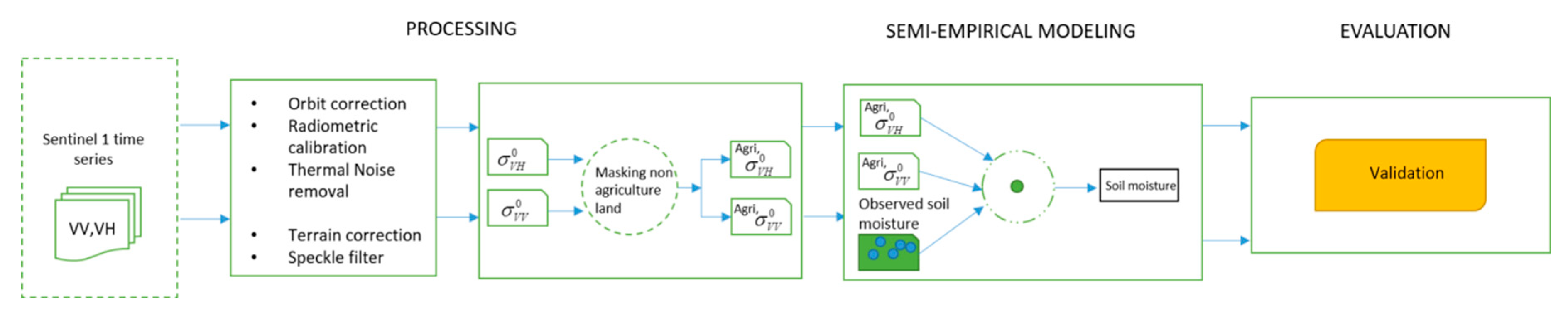
1. Introduction
Soil moisture estimation across space and time has become possible with the advent of microwave remote sensing [
1]. The amount of moisture in the soil is a function of physical, chemical, and management practices. Soil moisture is highly dynamic across space and correlated in time. The radar backscattering coefficient is a function of soil characteristics such as dielectric constant, texture, and surface roughness, and depends on the wavelength, polarization, and angle of incidence of the radar [
1]. Shorter wavelength C-band radar backscatter has shown sensitivity to surface soil moisture at a depth of about 5 cm [
2,
3,
4]. The launch of the Sentinel-1 mission of the European Space Agency has made a huge amount of C-band data acquired since 2014 from all over the Earth’s surface accessible. This opened up new perspectives on studying soil moisture in semi-arid regions, as was undertaken in Karnataka, India, in this work. Large scale soil moisture monitoring will provide greater insights into energy fluxes, which can result in improved meteorological and climatic projections [
5] that will provide critical inputs for agriculture.
There have been studies based on physical, empirical, and semi-empirical models that estimate soil moisture over bare soils through radar remote sensing [
6,
7,
8]. Physical approaches require many input parameters such as surface roughness and slope, which are not available under practical conditions [
8]. Empirical models are only data driven, whereas semi-empirical models, while being data driven, also support theoretical considerations. In soil studies, they are site-specific and generally valid for specific soil characteristics [
3]. Previous semi-empirical studies have considered single polarization to build a relationship between soil moisture and a backscatter model at 10 cm depth [
9] and estimated
with a root mean square error (RMSE) of 3–6% [
10,
11,
12] using C-band data. There have also been studies that have used the SAR interferometry technique and Sentinel-1 data to estimate soil moisture and compare them with in situ measurements [
13]. Even though SAR interferometry is less frequently used in the remote sensing community to estimate soil moisture, its advantage lies in its ability to disentangle moisture and terrain roughness contributions. Most SAR-based soil moisture estimation studies have covered small areas limited to a few hundred square kilometers [
11,
12,
13,
14,
15,
16,
17]. Estimating soil moisture over a wider area and at a higher resolution using SAR imagery will provide information on managing water resources and irrigation scheduling that can benefit a large number of farmers [
14].
The aim of this study was to estimate soil moisture in bare rice agricultural soils. While SAR images have been used to estimate rice phenology using X-band TerraSAR-X images [
15], there have been limited studies to estimate the soil moisture in bare rice agricultural soils using Sentinel-1 C-band images. Bare soils in Siruguppa are rice growing areas that lie bare after the rice crop has been harvested in March, with rice stubble and weeds that have dried up during summer (March–June). By the time the monsoon rains start, it is extremely critical to estimate the amount of soil moisture in the top 10 cm, which will help farmers decide when to start preparing the land and start sowing the next crop. Surface roughness, soil status, soil moisture, and crop residue distribution affect radar backscatter [
16]. It is well established that
is more sensitive to variation in soils and
is more suited to the identification of dry crop residue [
17]. Utilizing both together can improve the accuracy of soil moisture estimates [
18]. Nevertheless, soil moisture studies using
and
together, especially using Sentinel 1 SAR data, are limited. The need for such studies over significantly large agricultural fields is very important to study agriculture, water, and food security. The major goal of this study was to estimate soil moisture over bare soils using both
and
polarization and compare it with in situ measurements at a 10 cm (0–10 cm) depth. At the time of measurement, soil moisture to 10 cm is at the steady state and consistent across that top surface layer and therefore the C-band can be assumed to detect the top 10 cm layer. However, it is known that C-band SAR signals cannot penetrate to a 10 cm depth.
The contribution of standing stubble to total backscattering coefficient is comparable with that of the soil surface when the stubble has more than 75% water content. Backscatter coefficient decreases with a decrease in water content in the stubble. However, when the water content in the stubble is less than 40%, the contribution to the total backscattering coefficient is negligible [
19]. We investigated both localized and generalized linear models to try to disentangle the stubble and soil moisture contributions. The linear coefficients of localized models were derived using in situ data acquired on a specific Sentinel-1 day. In contrast, generalized models were built using all in situ measurements acquired in the study period, thus adding the temporal dimension to the analysis of Sentinel-1 data. The question we wanted to answer is: can semi-empirical models estimate soil moisture, getting rid of the stubble contribution to the backscattering coefficient? We tried to answer this question by studying the effects of each variable, time, and polarization, separately. A localized model does not take into account the temporal evolution of backscattering, while a generalized model includes the time variable when estimating the linear coefficients. Furthermore, for each model, it is possible to keep the polarimetric channels separated or merge them. In this work, we used a large dataset of in situ measurements of soil-moisture acquired across a 2-year period to answer the above question. The issues of the stability of results and of collinearity of data are crucial and will be used to assess the results of this experiment.
The rest of this paper is organized as follows:
Section 2 is devoted to materials and methods,
Section 3 to the results, and
Section 4 presents the discussion. Finally, a few conclusions are drawn in
Section 5.
4. Discussion
Accurate estimation of was envisaged using a linear equation of and radar cross section from bare agricultural soils. A thorough data collection campaign was undertaken during 2017 and 2018, synchronizing with the pass of the satellite. Bare soil areas were mostly post-harvest cropped areas with little or no crop residue, depending on the crop sown. In the study area, 50% of the agricultural land comprises rice cropped and irrigated from a seasonal stream. Sentinel-1 SAR, dual polarized imagery was used to estimate soil moisture over bare soils using a semi-empirical model. Model parameters were estimated using linear and multi-linear regression. Performance evaluation was conducted based on a 70:30 ratio of sampled points and low RMSE was found between the observed and estimated soil moisture, when a linear relationship between and was combined for 2017 and 2018.
4.1. Relationship between and with Observed Data
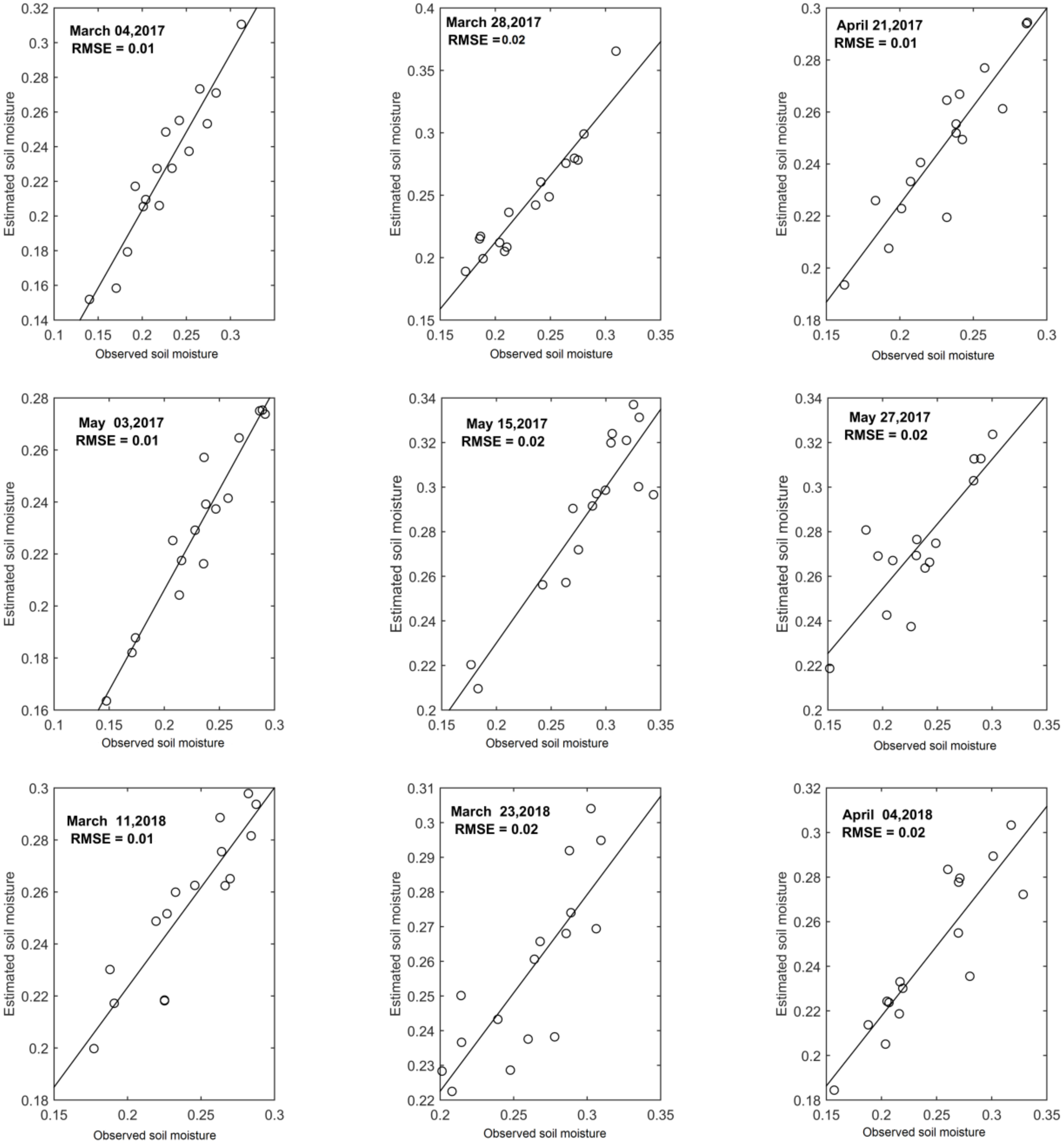
Soil moisture data were collected over two years (2017 to 2018) during the dry summer season from March to May from the 62 plots on the dates of the satellite passes. The relationship between
,
, and observed soil moisture by individual dates of the satellite pass (13 images) showed that in both years, the backscatter and observed soil moisture had a significant positive correlation [
2,
10,
27,
28]. In both years, VV polarization had a higher backscatter dB value than VH polarization. In cross-polarization (VH), signal attenuation occurs due to volumetric scattering [
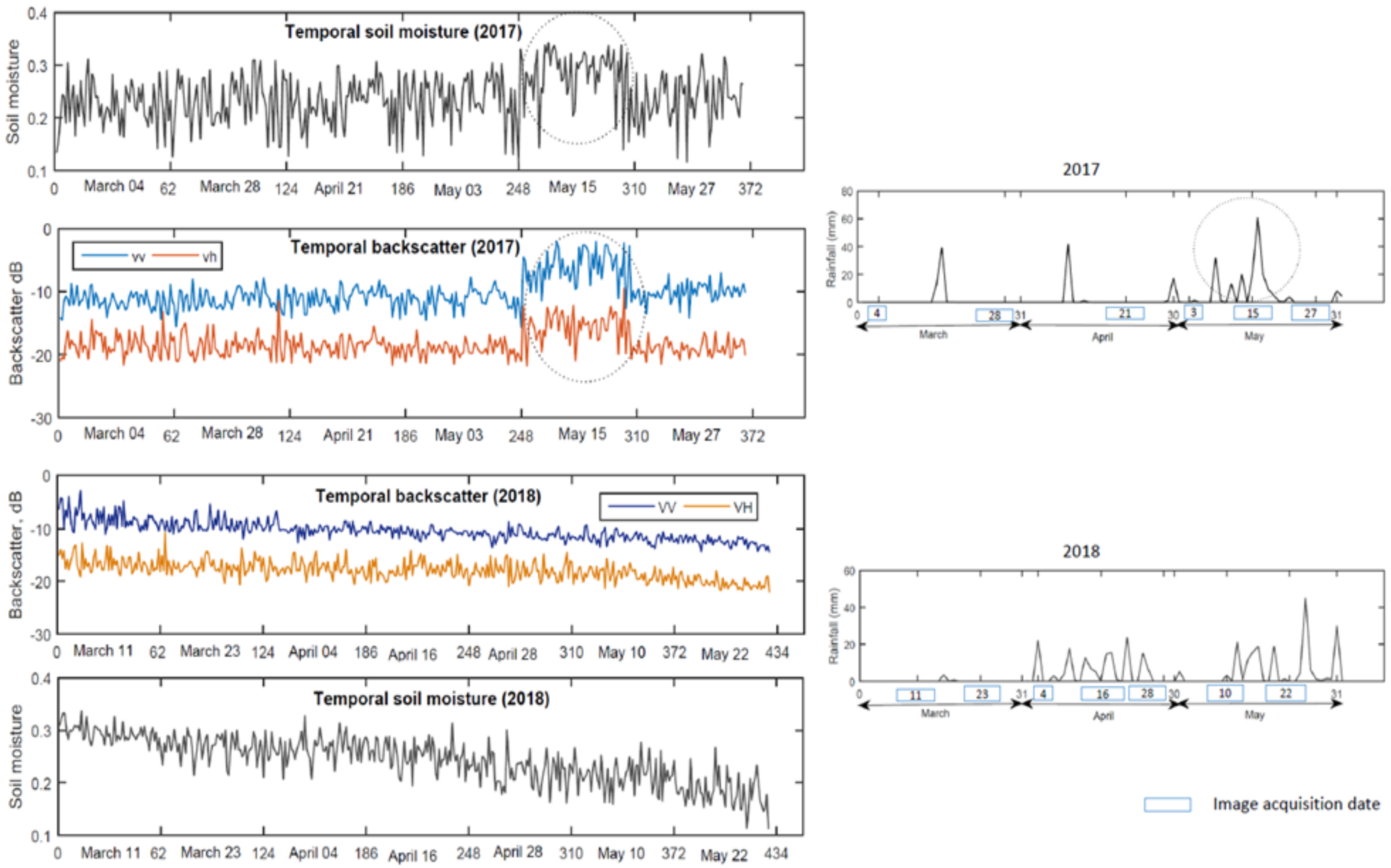
29]. In 2017, soil moisture constantly increased from 4 March to 27 April. The R
2 between radar backscattering coefficient and in situ measurements of soil moisture is reported in
Table 3. A sudden increase in R
2 (VV) can be observed on 15 May, corresponding to the consecutive rainfall events that occurred during the three days before the date of the satellite pass (
Figure 8). This means that there is a better correlation for high values of soil moisture, probably because under this condition, the radar backscattering coefficient’s dependence on soil moisture is more important than it is on surface roughness.
Similarly, an unexpected increase in
was observed (
Figure 5). 27 May 2017 (
Table 3) had a low R
2 value from
compared to the rest of the dates due to the rainfall event (
Figure 8), weeds or crop residue moisture [
24]. In 2018, R
2 for the relationship between
and observed soil moisture was significant during March because of residual soil moisture (i.e., the crop residual moisture influenced the radar backscattering coefficient,
Table 3). Residual soil moisture was low on 4 April and 22 May due to evaporative demand and higher between 16 April and 10 May due to consecutive rainfall events (
Figure 8). R
2 did not decrease from March to May, probably due to irregular changes in crop residue moisture, since
is sensitive to it [
24]. The R
2 values from
during March were relatively low despite no rainfall in the month because of residual soil moisture from the previous crop. The cumulative moisture due to rainfall during April is reflected in the low R
2 of 16 April and 28 April (
Figure 8). During May, high R
2 values were due to bare soils. A linear combination of
and
during each date in 2017 produced higher R
2 compared to R
2 from individual polarization. This shows that the addition of
and
or vice versa improves the backscatter and soil moisture relationship rather than a single relationship with different polarization (
Table 3). A similar relationship existed during 2018 from a linear combination of
and, which improved R
2 significantly (
Table 3).
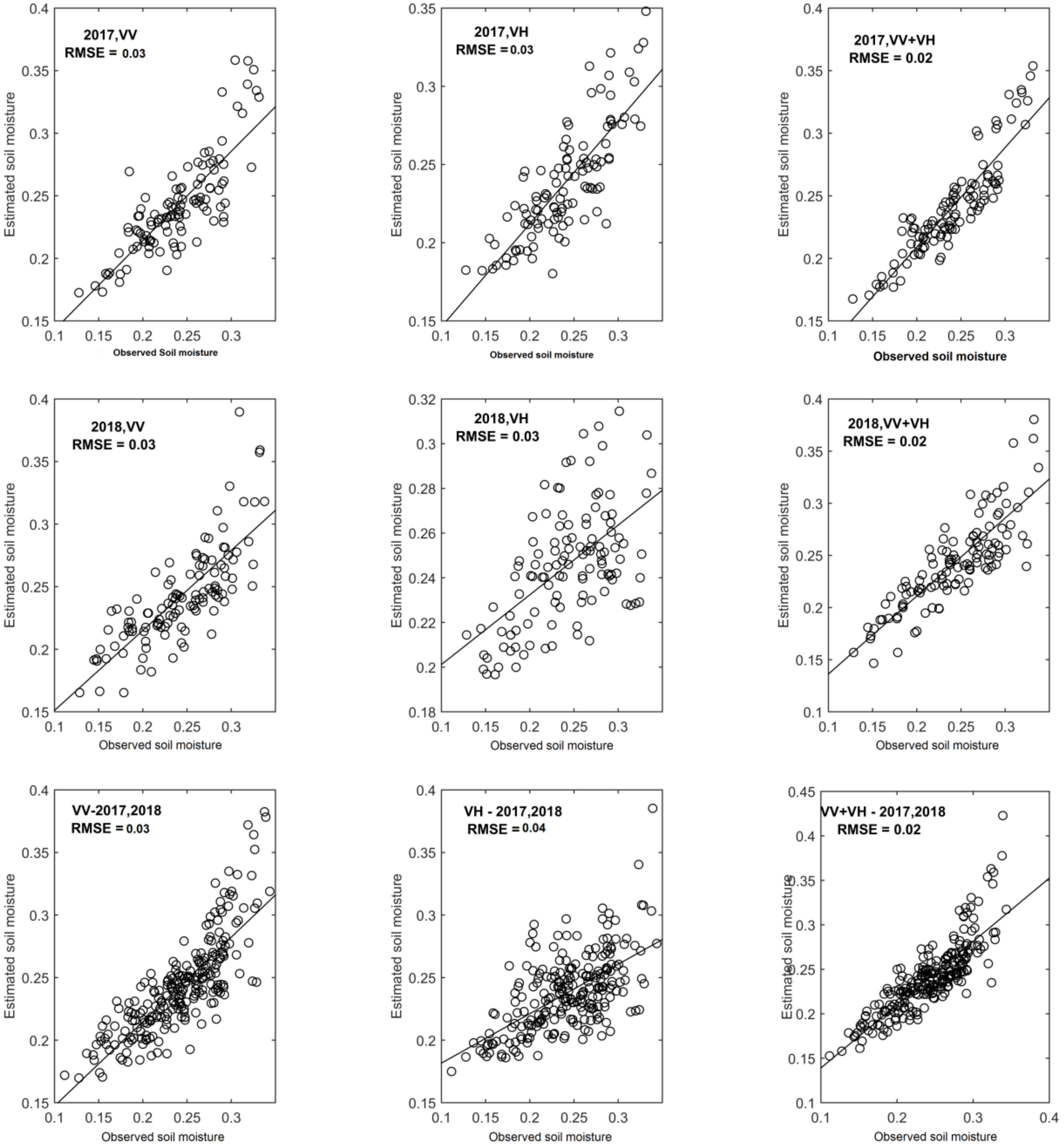
4.2. Localized and Generalized Relationships
To operationalize the accurate estimation of soil moisture for decision making, a global relationship was envisaged considering all dates during the dry season. The R
2 value of global relationship from VV polarization during 2017 was 0.68, which was higher than the mean of the local relationships. The generalized relationship was found to be more useful for an accurate soil moisture estimate. In addition, R
2 for the generalized relationship performed better than the mean of the localized relationship (0.67) with VH polarization. The scenario during 2018 from VV polarization was more influenced by rainfall events in the dry season. The R
2 values ranged from 0.56 to 0.69 with a mean of 0.62 from localized relationships and 0.66 from the generalized relationship, which was more than the local mean. R
2 was very low from VH polarization due to cumulative moisture from rainfall events. However, the generalized relationship produced a lower R
2 than the mean localized relationship for VH in 2018 (see
Table 3 and
Table 4). The usefulness of a generalized relationship was exhibited with a consistent increase in the accuracy of the soil moisture estimates over two years. The relationship from VV and VH polarization during 2017 showed significantly lower R
2 than the linear combination of VV and VH during the same year. Similarly, also during 2018, R
2 was significantly higher than the individual polarization. Finally, the best relationship was obtained when the linear combination of two polarizations was combined (appended) for the two years 2017 and 2018, than from single polarizations combined for the two years. It was inferred that generalized relationships are more promising in terms of building a model compared to localized relationships, which may not relate to the entire population.
4.3. Modeling the Relationships
The relationships of localized and generalized modeling were explored and tested for multicollinearity, especially linear combination models
+
. Multicollinearity is a statistical phenomenon in which two or more predictor variables in a multiple regression model are highly correlated [
30]. To detect multicollinearity, we used an indicator called variance inflation factor (VIF), which is a tool to measure and quantify how much the variance is inflated [
30]. If any of the model’s VIF values exceed 5 or 10, it is an indication that the associated regression coefficient is poorly estimated because of multicollinearity [
31]. The P value indicates statistical significance for independent variable contribution in the model, which is explained in
Section 2.4.3.
For generalized models, nine different types of linear relationships were explored with
and
data (
Table 6) during 2017 and 2018. In 2017, among the three possible models
,
and,
+
, individual models
and
showed a low RSE and the
p value was statistically significant. When
was added to
, the RSE was lower than in the individual models. This indicates a very good relationship with a low VIF as well as
p value for both backscatter coefficients. Similar results were observed in 2018. Generalized models derived by combining two years (2017 and 2018) of data showed similar results as individual year models. This study also showed that the linear combination equations from the localized models also performed well with low VIF (<2) and a
p value statistically significant for both backscatter coefficients (
Table 7 and
Table 8).
A collinearity test on the generalized and localized models showed that the VIF for a linear combination of both backscatter coefficients (VV + VH) was <3. Hence, these models are non-collinear. All models showed low p value, indicating that both backscatter coefficients made meaningful addition to the models. During modeling relationships with a linear combination of individual backscatter coefficient, it was inferred that the individual backscatter coefficients were non-collinear, contributing to R2 independently. It was found that the localized models from individual dates varied over time, and any one equation with a low RSE and VIF may not represent the whole season. In addition, the generalized models produced lower RSE representing the whole season, and were hence better than each localized model.
4.4. Validation of Models
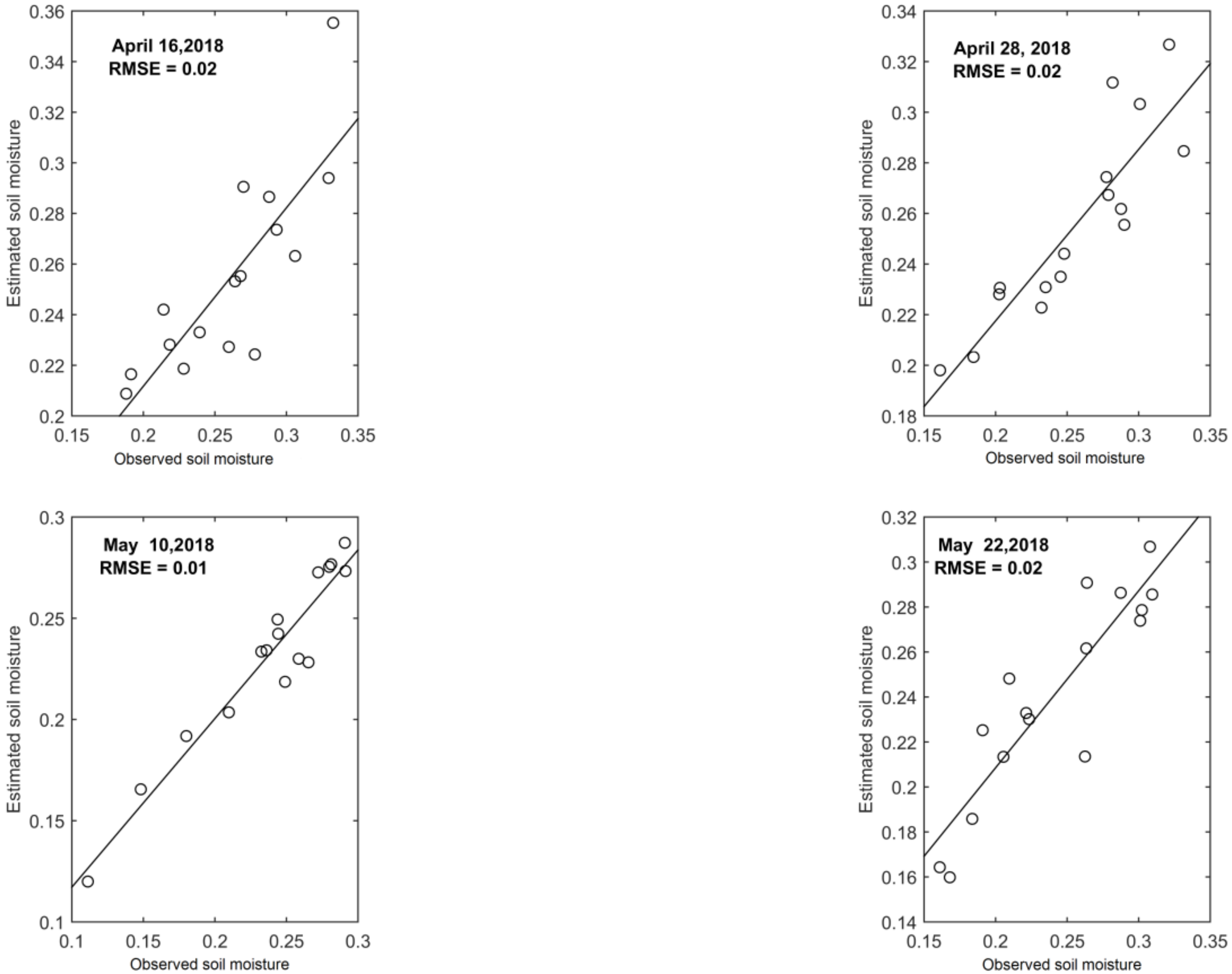
Models were validated using 30% of the sampled points. Results for the localized models are summarized in
Table 5. In 2017, the lowest RMSE (0.01) was found on 21 April.
Figure 8 shows that no rainfall or very weak rainfall was observed on this day. An increase in RMSE was observed on 15 May. Similarly, in 2018, the lowest RMSE was observed on 23 March and the highest (0.03) on 16 April 2018, probably due to the increase in rainfall. The results seem to show that the RMSE of the models is related to the amount of rainfall. Localized models performed better in drier soils.
As far as the generalized models are concerned, the validation results showed that generalized models obtained using co-polar
data provided a lower RMSE than those based on cross-polar
data for both 2017 and 2018 and taking all data acquired from 2017 to 2018. We also found that the linear combination of both co-polar and cross-polar backscattering coefficients always provided a lower RMSE than the models using only one polarization. The best results came when using the linear combination of polarizations and all the data acquired along the two years, resulting in an RMSE of 0.02 (
Table 6). This globalized model was used to produce maps of soil moisture and its spatial variability (
Figure 9,
Figure 10 and
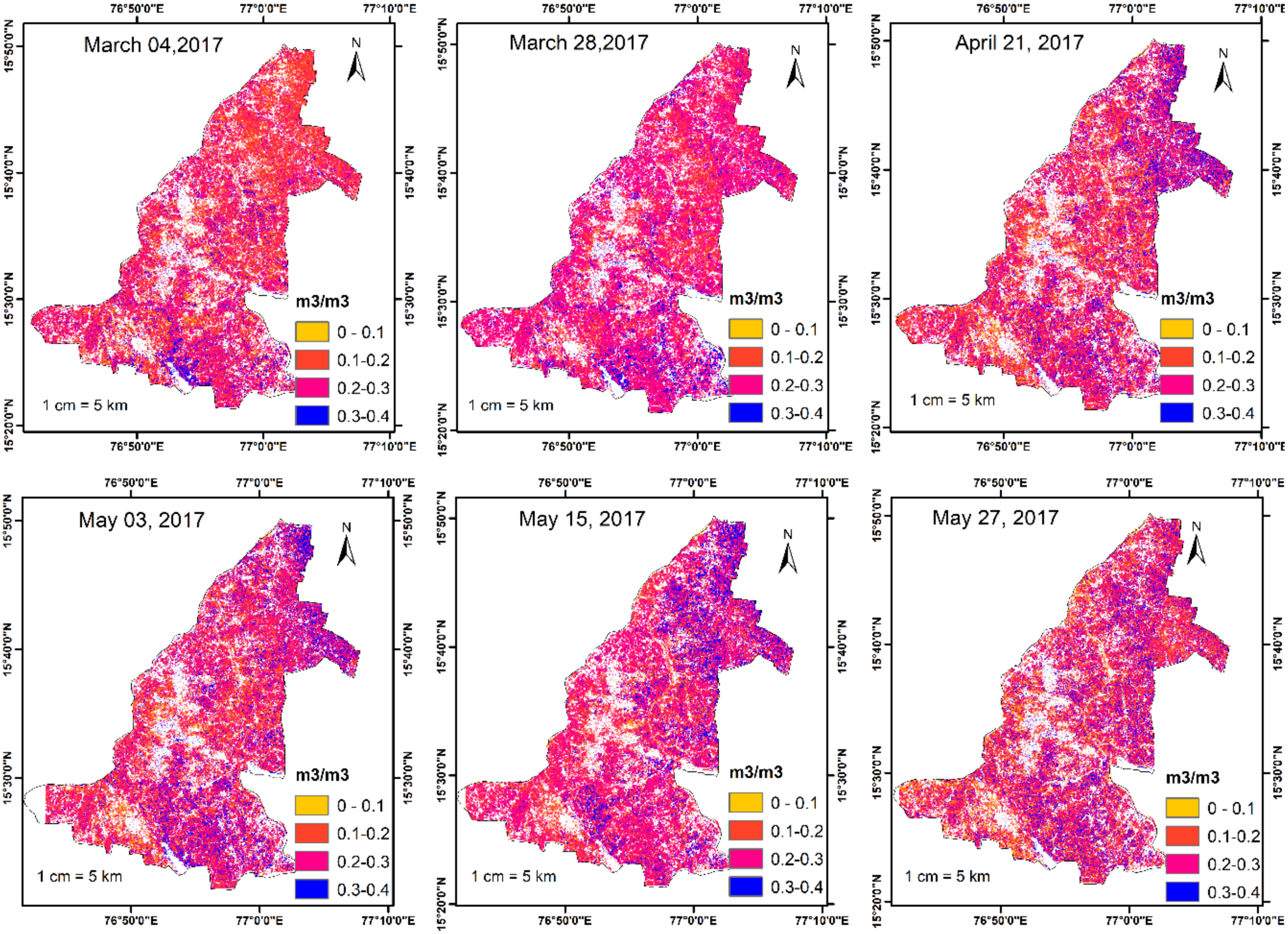
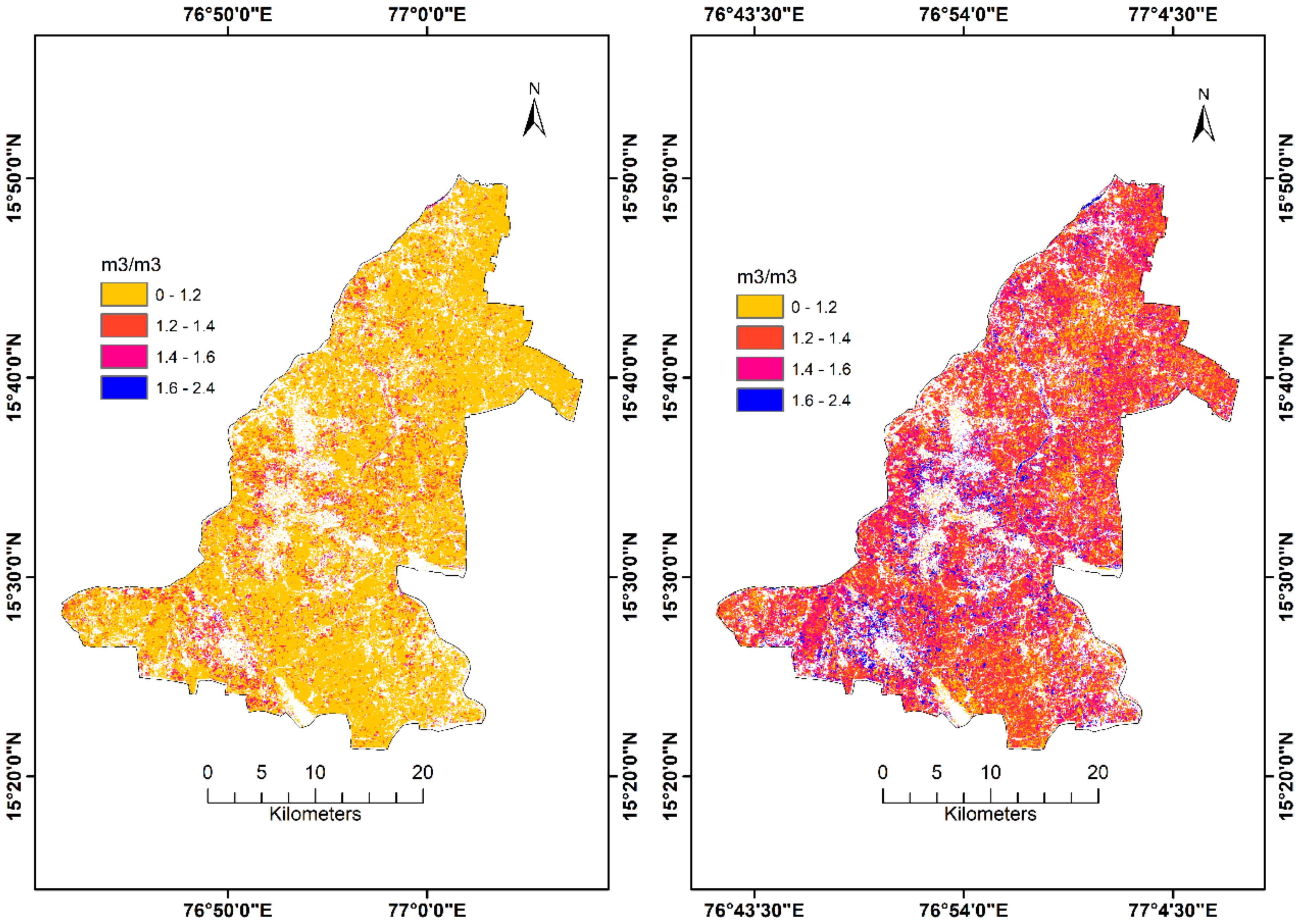
Figure 11). This is probably the most important result, as a simple multi-linear model using both co-polar and cross-polar Sentinel-1 data acquired over long time periods can reproduce the spatial variability of soil moisture.
5. Conclusions
This study aimed to accurately estimate the soil moisture of bare, post-harvest agricultural areas collected from Siruguppa taluk (sub-district) in the Karnataka state of India. Fifty percent of this agricultural area is grown with rice that is irrigated by seasonal canal irrigation. An accurate estimate of volumetric soil moisture () was envisaged using a semi-empirical model based on a linear equation of co-polarized and cross-polarized radar cross section obtained by Sentinel-1 images. A thorough data collection campaign was undertaken during 2017 and 2018 during the pass of the satellite.
Both localized and generalized models were developed using Sentinel-1 image independently and all images together, respectively. Results indicate that the accuracy of the soil moisture estimates increased when using both co-polar and cross-polar images instead of only or , independently.
The use of localized models revealed that the RMSE of soil moisture estimates decreased corresponding to dry periods, with little or no rainfall. This indicates that better estimates of soil moisture can be obtained for drier soils. Coming to globalized models, soil moisture estimates with lower RMSE were observed when merging all data acquired in 2017 and 2018, and co-polar and cross-polar images, with a R2 of 0.7 and RMSE of 0.02. The availability of a large amount of in situ data collected over a large area demonstrated that a generalized linear model based on the joint use of co-polar and cross-polar C-band SAR images acquired for a long time period, with a short revisiting time of twelve days, could capture spatial variability in soil moisture. This is an important result as the availability of Sentinel-1 data can provide farmers with timely and accurate estimates of soil moisture and enable the mapping of its spatial variability by using simple semi-empirical models. This information, when provided in the immediate weeks and months preceding the cropping season, could be very crucial in determining planting dates and assessing early season plant growth, thereby playing a key role in influencing productivity.


