1. Introduction
Soil moisture (SM) is an essential hydrologic variable that impacts evaporation, infiltration and runoff, playing an important role in energy and carbon exchanges [
1]. Its influence is assessed over a range of different scales: crop scale [
2], hydrological scale [
3], meteorological scale [
4] and climatic scale [
5]. Hence, the majority of hydrological and agricultural applications require high, at least at 1 km, resolution SM data [
6,
7,
8]. Surface SM observations are nowadays provided on a global basis using remote sensing data. Among all existing satellites, passive L-band microwave sensors are widely used to derive SM thanks to the strong physical link between the brightness temperature and the 0–5 cm SM profile [
9,
10]. The downside to the operational retrieval of SM from microwave observations is given by the low resolution (LR) of the products, which ranges from 40 to 60 km [
11,
12], a resolution that is too coarse for most hydrological and agricultural applications [
13,
14]. Alternatively, optical/thermal sensors have the advantage of providing data at medium and high resolutions. In particular, Landsat and ASTER (Advanced Spaceborne Thermal Emission and Reflection radiometer) have resolutions of several tens of meters, while MODIS (MODerate Resolution Imaging Spectroradiometer) has a resolution ranging from 250 to 500 m and to 1 km, depending on what band is used. Even though optical data could be used to derive SM, the main drawback in deriving a retrieval methodology is given by the sensors’ sensitivity to meteorological conditions (including cloud presence) [
15,
16,
17] and vegetation cover [
15,
18]. More recently, the potential of Synthetic Aperture Radar (SAR) satellite data has also been investigated in deriving SM products. In particular, [
19,
20,
21] have investigated the potential sensitivity of C-band and L-band SAR data with respect to SM, with results showing the higher potential of L-band over C-band, due to its higher penetration depth. The main advantage of using SAR data is the high resolution it provides (several tens of meters). However, the main drawback is that it is difficult to account for the soil roughness and the vegetation backscattering effect in the soil moisture retrieval modeling [
20,
21,
22].
However, a synergy between the LR microwave and high resolution (HR) optical/thermal data [
23] can be used in order to derive SM at various spatial scales. This is achieved by using the optical-derived land surface temperature (LST), which is linked to the soil water content and vegetation cover [
24,
25]. Most of the methods based on the synergy between microwave and optical data generally use the triangle [
24] or trapezoid approach [
26], in which the variations in LST are linked to variations in soil water content and vegetation cover [
27,
28]. The main hypotheses behind the triangle and trapezoid approaches are: (i) the only variability factors of the LST are the vegetation cover, surface SM and vegetation water stress, (ii) uniform meteorological conditions are met over the study area and (iii) the extreme temperatures can be correctly interpolated from the LST–NDVI (Normalized Difference Vegetation Index) space, which implies a heterogeneity of the surface conditions at the observation resolution [
29,
30]. As classified in [
16] and in [
17,
31], there are various methodologies based on the synergy between microwave and optical data: polynomial fitting methods, evaporation-based methods, the UCLA method [
32], the Peng method [
33], thermal inertia-based methods [
25,
34,
35]. The polynomial fitting methods [
23,
36], considered as purely empirical algorithms, use a polynomial function of LST, NDVI and surface albedo to express SM. Studies like [
37,
38,
39,
40] also take into account the brightness temperature in the polynomial fitting model in order to derive SM at 10 and 1 km resolutions from SMOS observations.
The evaporation-based methods are more theoretically and physically based than the polynomial fitting approach [
16,
17]. In these models, the evaporative fraction (EF) and/or the soil evaporative efficiency (SEE) are used as SM proxies, due to (i) keeping a constant value during the day [
41,
42], and (ii) their direct link to SM, while being independent on incoming radiation, as opposed to evapotranspiration or LST [
43]. The SEE, defined as the ratio of actual to potential evaporation, can be derived either using microwave SM data or using optical data. Through its link with SEE, evaporation is the physical process that allows a link at multiple resolutions between the microwave SM and optical data. In particular, these models represent the spatial link between optical-derived SEE and surface SM. Their main advantages over the polynomial fitting methods are that (i) they are self-calibrated for each SMOS pixel individually, which fosters the validity of the hypothesis of meteorological uniformity even compared to methods implementing adaptive windows [
40,
44] and (ii) the average of the estimated HR SM is equal to the LR observed SM (meaning that the error residual as termed in [
44] is zero).
Although the hypothesis of meteorological uniformity at large scale is difficult to be met by the methods based on the triangle or trapezoid models [
44], recent studies have tackled that issue by introducing a self adaptive window in the downscaling methodology, which better meets the atmospheric forcing hypothesis. [
44] have introduced a self-adaptive window in a downscaling method of SMAP SM and applied it over the Iberian Peninsula. [
40] have implemented an adaptive moving window in the polynomial method developed in [
45] and applied it to SMOS data over the Iberian Peninsula and Australia. The adaptive window in [
40] had a radius of 9 SMOS pixels, while [
44] used an adaptive window of different sizes and compared the results obtained with fixed window sizes from 4 to 7 SMAP pixels. The sizes considered in both studies allowed minimizing the regression residuals compared to using a larger spatial extent.
The algorithm presented in [
46] was improved in [
18,
47]. DISPATCH (DISaggregation based on a Physical and Theoretical scale CHange) converts HR MODIS-derived SEE fields into HR SM fields by expanding a first order Taylor series of a SEE model around the LR SMOS SM. The HR SEE fields are derived using HR LST and NDVI data and the LR extreme temperatures, which are estimated from the LST-NDVI feature space [
26,
47]. Optical data are then linked to SM by using a self-calibrated SEE(SM) model [
15]. DISPATCH also meets the meteorological forcing hypothesis, as it is self-calibrated at the SMOS pixel scale, where uniform atmospheric conditions are generally fulfilled, and can therefore be applied at large scales [
15,
48,
49].
The current SEE(SM) model used in DISPATCH is linear; however, multiple studies have noted a strong nonlinear relationship between the microwave-derived SM and the optical-derived SEE [
50,
51,
52]. The model provided in [
51] has previously been implemented over the Australian landscape by [
46,
53], by testing the DISPATCH approach at 10 and 4 km resolutions, respectively. They both used the nonlinear model in a second order disaggregation scheme of the SM data derived from the National Airborne Field Experiment, with satisfying results being reported. However, the impact of the nonlinear relationship between SEE and SM needs further investigation, in different surface conditions and at different resolutions, since this has not been addressed in previous studies. In particular, the nature of the model used within DISPATCH depends on the calibration strategy, and to date, there is no study analyzing the SEE(SM) calibration in both time and space.
Most of the thermal-based disaggregation techniques use a daily calibration of their parameters. In [
36], a linkage model calibrated on a daily basis, combined with high resolution NDVI, surface albedo and LST, is applied to data acquired from the Special Sensor Microwave Imager (SSM/I) and Advanced Very High Resolution Radiometer (AVHRR) in order to derive high resolution SM estimates. In [
37,
45], a linking model is used to relate SMOS SM to MODIS NDVI and LST through regression coefficients, which are calibrated on a daily basis. The algorithm was also applied to SMOS and MSG (Meteosat Second generation) SEVIRI (Spinning Enhanced Visible and Infrared Imager) observations to derive 3 km resolution estimates over Spain and Southern France [
38]. The same model is used by [
39], with four different water indices formulations, in order to derive 500 m resolution soil moisture from SMOS and MODIS observations. A polynomial downscaling methodology is used in [
54], with regression coefficients calibrated for every day over the observed scene, in order to derive HR SM estimates from AMSR-E (Advanced Microwave Scanning Radiometer on the Earth Observing System) and MSG SEVIRI observations. The UCLA method [
32] uses a linear relationship to connect a soil wetness index with SM, index derived on a daily scale. In a similar manner, [
33] use the VTCI (Vegetation Temperature Condition Index) instead of the soil water index in their downscaling methodology, which is derived on a daily basis by rescaling the LST of each pixel between two extreme LST values, per NDVI interval. The thermal inertia method is used by [
25] to relate daily averaged SM estimates to diurnal changes in the soil temperature, calibrating their model on a monthly basis in order to reduce the impact of vegetation biomass on the estimates [
17]. In this context, this study aims to improve the robustness of the SEE(SM) model used within the DISPATCH methodology and hence the accuracy of the disaggregated dataset. In this respect, this study implements the nonlinear SEE model developed by [
51] in addition to the classic linear model (used in the current DISPATCH version) to disaggregate SMOS Level-3 SM down to 1 km resolution, over a range of different conditions. The impact of the calibration of each (linear and nonlinear) model is investigated. In practice, the linear and nonlinear models are calibrated on a daily and on a multi-date basis, and a comprehensive assessment is performed.
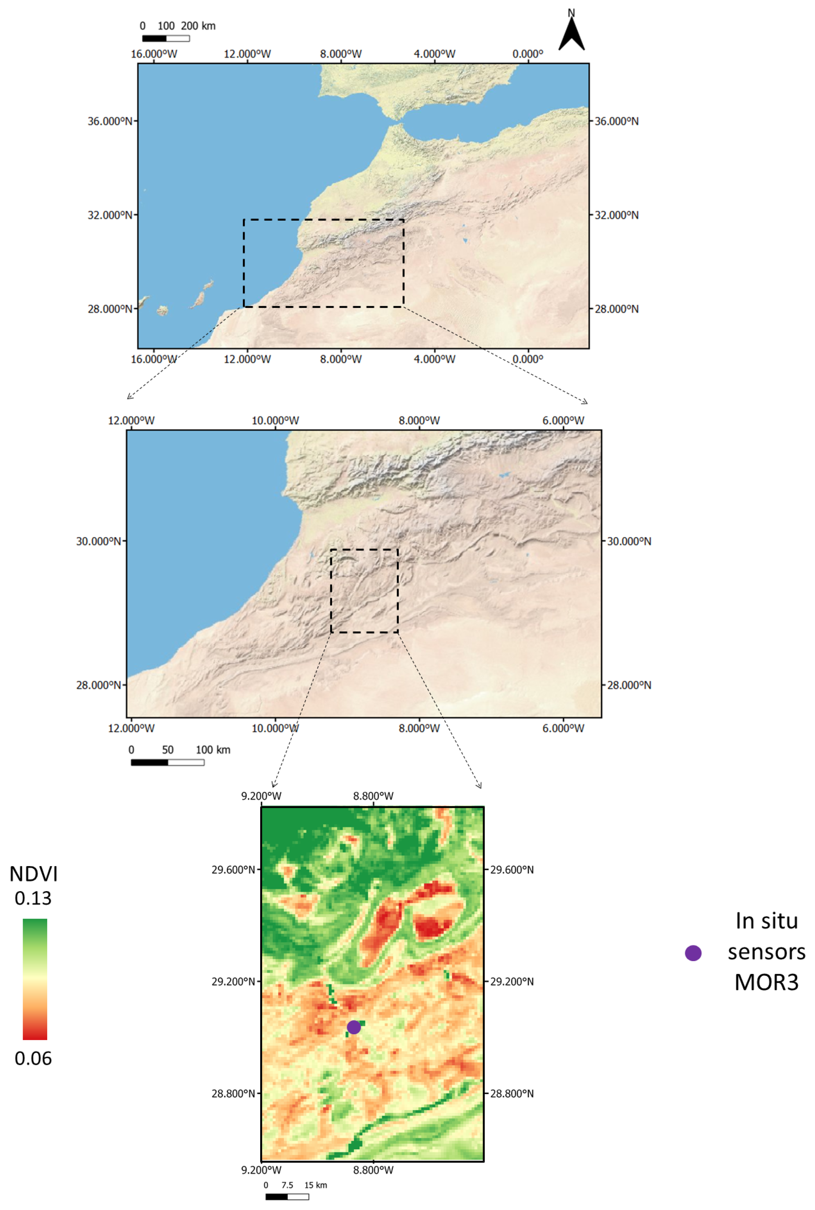
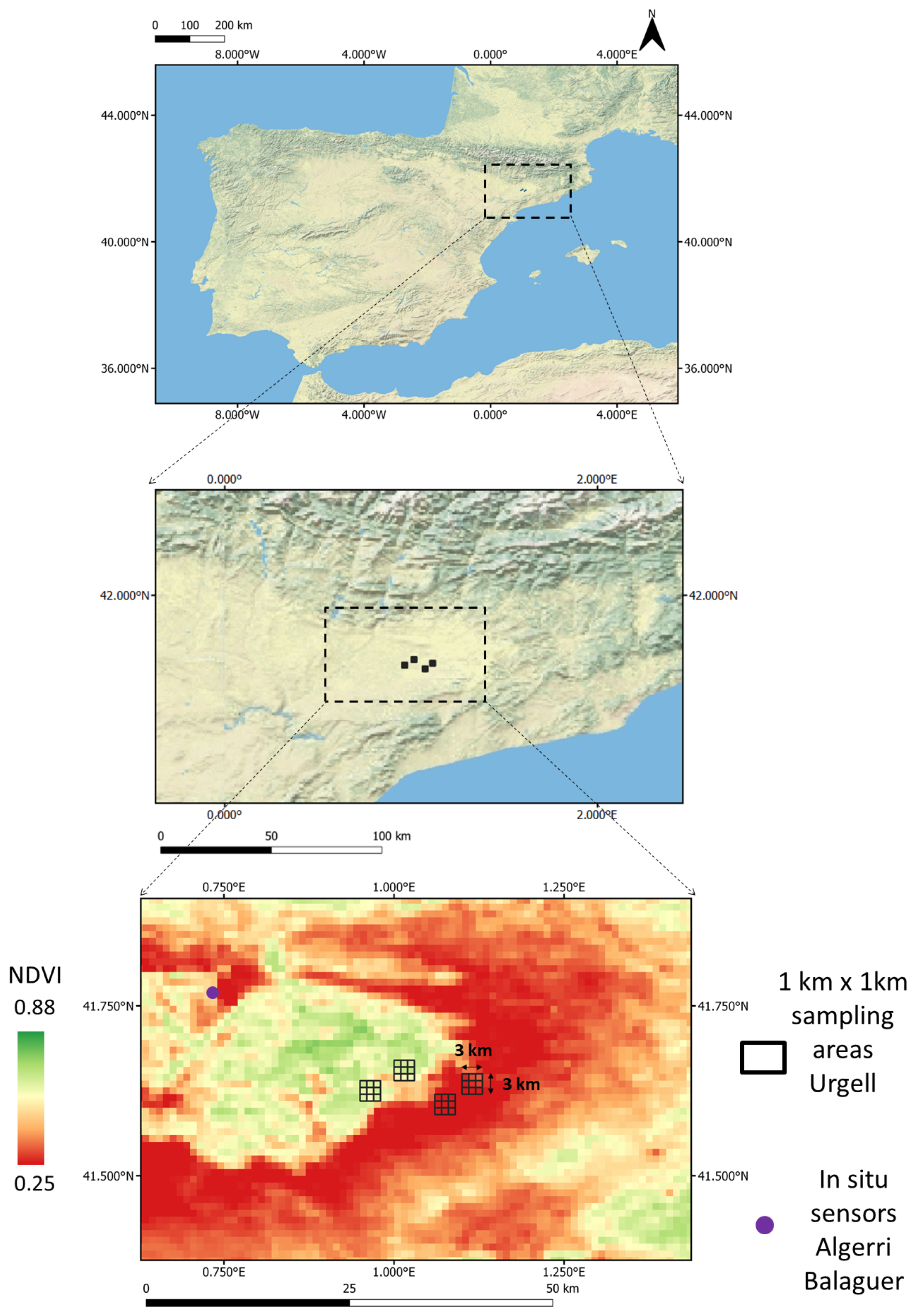
The approach is validated using in situ SM measurements for three different areas: over a mixed dry and irrigated area in Urgell, Catalonia, Spain (2011 and 2015), over an irrigated area in Algerri-Balaguer, Catalonia, Spain (2017–2018) and over a dry area in Morocco (2016–2017). The study sites along with all the data are presented in
Section 2. In
Section 3, the DISPATCH algorithm is briefly presented, along with the two SEE(SM) models.
Section 4 offers a comparison between the disaggregated SM estimates.
4. Results and Discussion
In this section, the performance of the linear and nonlinear models with the daily and multi-date calibrations is assessed in terms of disaggregated SM values. Two types of validations are performed: a spatial validation on a daily time scale and a spatio-temporal validation. More specifically, the disaggregated SMOS SM using both the linear and nonlinear models, in both calibration modes, are compared against in situ measurements, for each study area separately. The reasoning behind doing two types of validation is that on the one hand, the spatial validation is the type of validation to perform in order to evaluate the disaggregation methodology. On the other hand, this can only be done for Urgell 2011 and 2015. Since the measurements for Urgell are short in time, we performed a temporal validation by adding Algerri Balaguer and MOR3, the latter site being added in order to test DISPATCH in an area that is not suitable for disaggregation (i.e., arid area).
4.1. Spatial Validation
A spatial validation was performed at the daily time scale for Urgell 2011 and Urgell 2015, to evaluate the spatial representation of the DISPATCH SM at the sub-SMOS-pixel scale. As mentioned in [
18], this type of validation is particularly useful for disaggregation methodologies, as it allows to separate the spatial and temporal trends provided by SMOS and by DISPATCH.
Table 2 shows the range (considering all days) of the correlation coefficient, slope of linear regression, bias and uRMSE obtained for Urgell 2011, taking into account both models and calibrations. For each range interval, the mean value (simple average for all days) of correlation, slope, bias and uRMSE.
Table 3 shows the same statistics obtained for Urgell 2015.
4.1.1. Daily Calibration
When doing a spatial validation in the daily calibration mode, the results obtained with the nonlinear model are slightly better than the one obtained with the linear model in the case of Urgell 2011, whereas for Urgell 2015, the linear model performs better.
When comparing at the daily time scale, the linear model gives better correlation values than the nonlinear model in the case of Urgell 2015, with an average value of 0.59 as opposed to 0.09. In the case of Urgell 2011, the results are comparable: a mean of 0.12 (linear model) and 0.11 (nonlinear model), with ranges of [−0.21; 0.44] and [−0.26; 0.49], respectively.
In the case of the slope of linear regression, the results are also similiar over Urgell 2011: a mean of 0.05 (linear model) and 0.06 (nonlinear model). Nevertheless, the range of the nonlinear model is slightly better than the range of the linear model: [−0.05; 0.25] as opposed to [−0.05; 0.14]. In the case of Urgell 2015, the linear model is superior to the nonlinear model, with a mean slope of 0.47 as opposed to −0.04.
Low values of bias have been obtained using both models. In the case of Urgell 2011, the values of the mean bias is ∼−0.1 m/m for both models, while for Urgell 2015, a lower mean bias is obtained with the linear model: −0.027 m/m as opposed to −0.070 m/m.
Low values of uRMSE have been registered, which in general are slightly lower when using the linear model for both sites: a mean value of 0.066 for Urgell 2011 and 0.068 for Urgell 2015.
4.1.2. Yearly Calibration
When looking at the yearly calibration mode, the nonlinear model further improves the correlation coefficient: a mean value of 0.17 is obtained for Urgell 2011 and 0.66 for Urgell 2015.
The bias remains roughly the same, with a mean value ∼−0.010 m/m for Urgell 2011 and −0.023 m/m for Urgell 2015, comparable with the values obtained with the linear model with a daily calibration.
However, when comparing both models in all calibration modes, the nonlinear model in the yearly calibration mode systematically improves the results. In the case of Urgell 2011, the range of correlation coefficients is improved from [−0.26; 0.49] (nonlinear model, daily calibration) to [−0.23; 0.57]. In the same manner, the higher end of the range of the slope of linear regression is also improved from 0.25 (nonlinear model, daily calibration) to 0.42. In the case of Urgell 2015, the range of the correlation coefficient improves from [0.40; 0.75] (linear model, daily calibration) to [0.57; 0.81], while the lower limit of the range of the slope of linear regression increases from 0.18 (linear model, daily calibration) to 0.36.
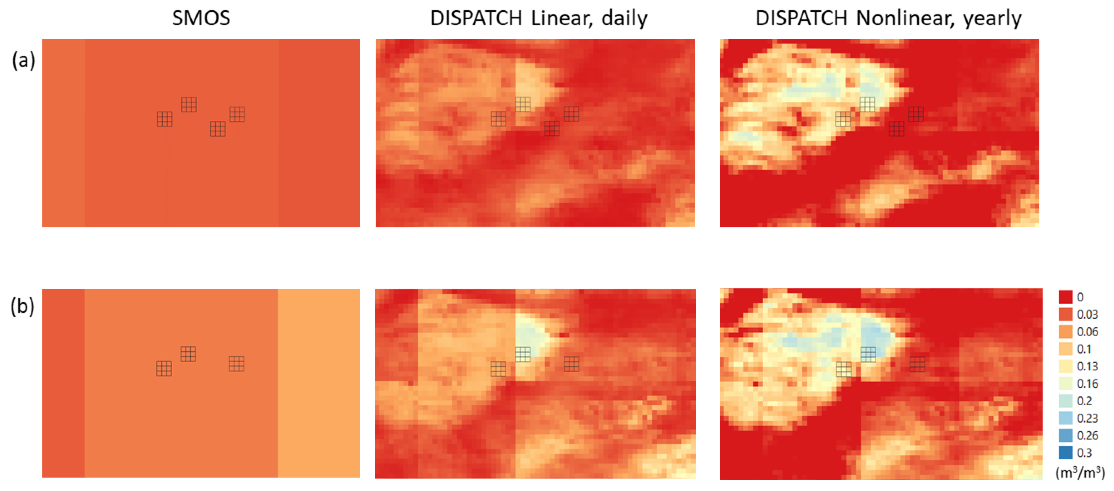
In general, better correlations have been found for both the linear and nonlinear models on sampling dates with larger spatial variability in the SM measurements. One such example is presented in
Figure 3, which shows a visual representation of the SMOS and DISPATCH SM (in linear mode with daily calibration—current operational version of the algorithm, and in the nonlinear mode with yearly calibration—the combination that yields the best results over the area). Results are shown for DOY 196 (year 2011) and DOY 223 (year 2015). One can observe that compared to the SMOS SM, both DISPATCH products better capture the spatial variability within the area, distinguishing between the dryland and the irrigated area. Moreover, the variability is higher in the case of the nonlinear model with a yearly calibration.
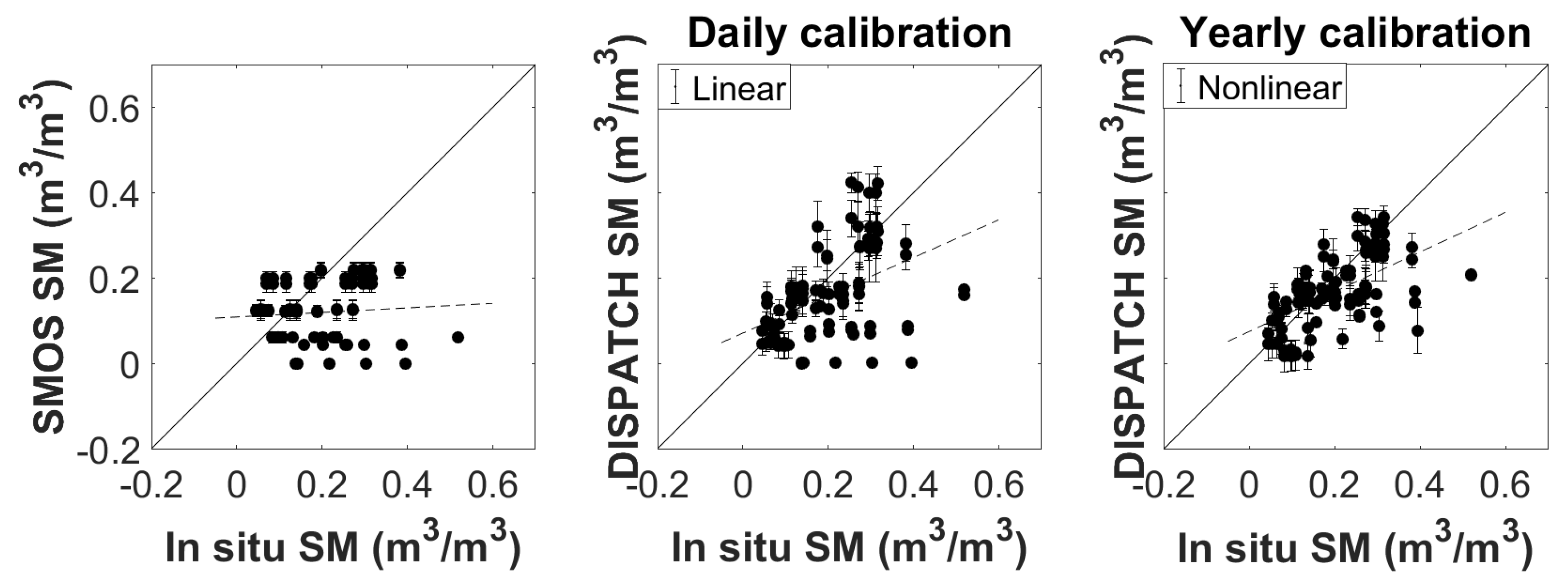
In the same manner as for
Figure 3,
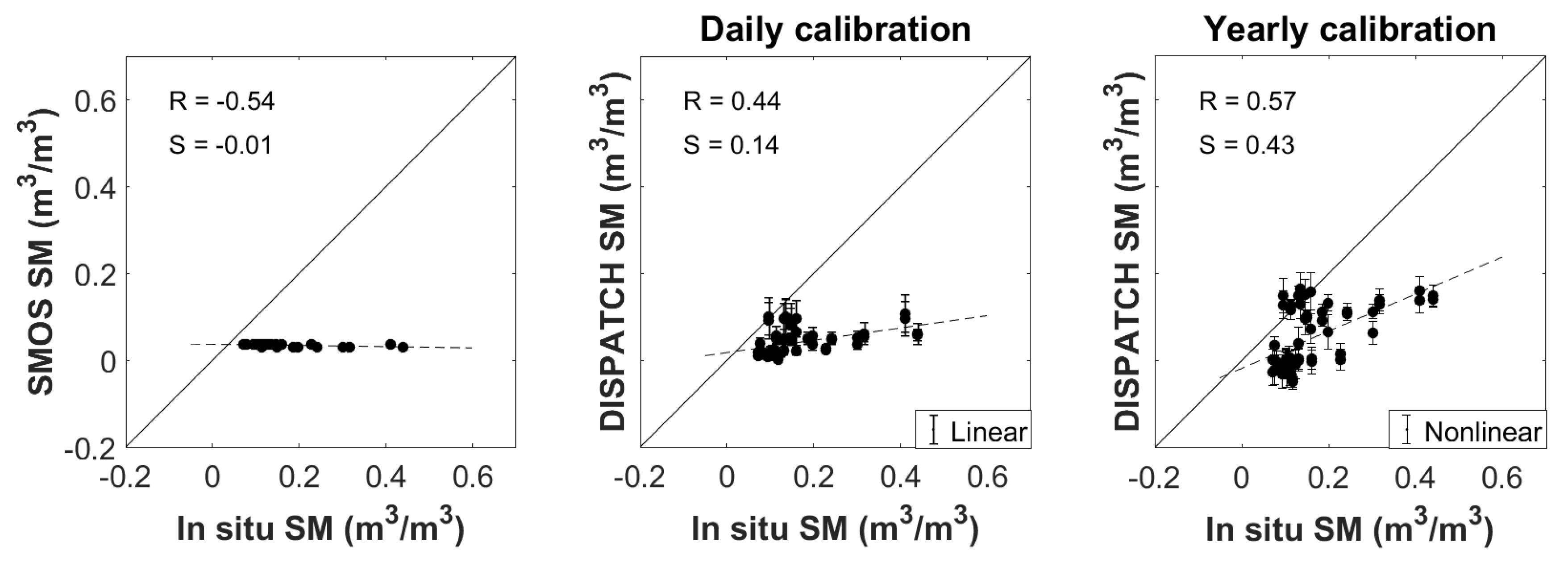
Figure 4 shows the SMOS SM and the DISPATCH output with respect to in situ measurements for DOY 196 (year 2011), while
Figure 5 shows the SMOS SM and the DISPATCH output with respect to in situ measurements for DOY 223 (year 2015). The error bars present in the plots represent the standard deviation. It is reminded that the in situ dataset corresponding to Urgell (collected by gravimetric measurements) was aggregated at a 1 km scale by simple linear averaging, for the sampling days. The DISPATCH output presented corresponds to the linear SEE(SM) model with the daily calibration mode, and to the nonlinear SEE(SM) model with the yearly calibration mode.
The correlation coefficient is improved from −0.54 (SMOS) to 0.44 (linear model, daily calibration) and to 0.57 (nonlinear model, yearly calibration) for DOY 196 (year 2011), while the slope of linear regression also increases from −0.01 to 0.14 and 0.43, respectively. In the case of DOY 223 (year 2015), the correlation coefficient increases from −0.31 to 0.40 and 0.57, respectively, while the slope of linear regression is improved from −0.02 to 0.18 and to 0.36, respectively.
Even though better correlations have been found on sampling dates with larger spatial variability in the SM measurements, however, if the spatial variability is relatively large (due to the irrigated area), the linear model is less effective than the nonlinear model, as the nonlinearity effects of the SEE(SM) relationship become more apparent [
65]. In terms of the slope of linear regression, [
66] have shown it is a good indicator of the efficiency of the downscaling technique. In our case, the slope of the linear regression is systematically increased by the nonlinear model with the multi-date calibration, indicating it disaggregates the SMOS SM in a more effective way than the other model-calibration options. Another aspect to be taken into account is that the uncertainty in the downscaled SM when using a daily calibration might be associated with uncertainty in the daily retrieved parameters. This coupled with the nonlinear model being able to better capture the nonlinearity effects inherent to the SEE might explain the better performance of the nonlinear model in the daily calibration mode over Urgell 2011. In the case of Urgell 2015, the validation is performed over areas containing more pixels in the irrigated zone, and there seems to be compensation effects in the case of the linear model with the daily calibration, making it better suited than the nonlinear model with a daily calibration.
4.2. Spatio-Temporal Validation
As mentioned at the beginning of
Section 4, although the spatial validation is best suited to analyze the performance of the disaggregation methodology, the measurements for Urgell only span several days. Hence, we perform a temporal validation by adding two new sites: Algerri Balaguer and MOR3. We also include Urgell 2011 and 2015 in the temporal validation. Statistical results in terms of correlation coefficient, slope of linear regression, bias and unbiased root mean square error (uRMSE) between satellite and in situ SM are reported in
Table 4,
Table 5,
Table 6 and
Table 7 for Urgell 2011, Urgell 2015, Algerri Balaguer and MOR3, respectively. In each case, DISPATCH is tested with the linear and nonlinear modes, with both daily and multi-date calibrations. The sample size used in each analysis is also mentioned.
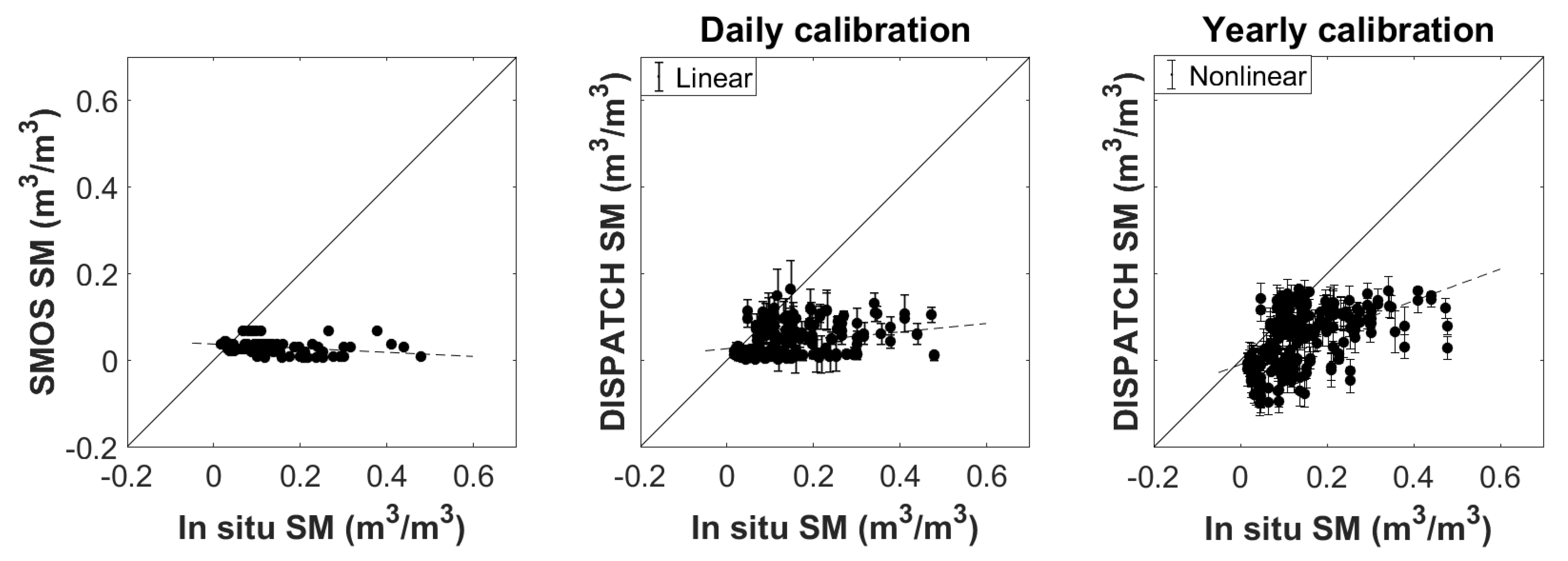
Figure 6,
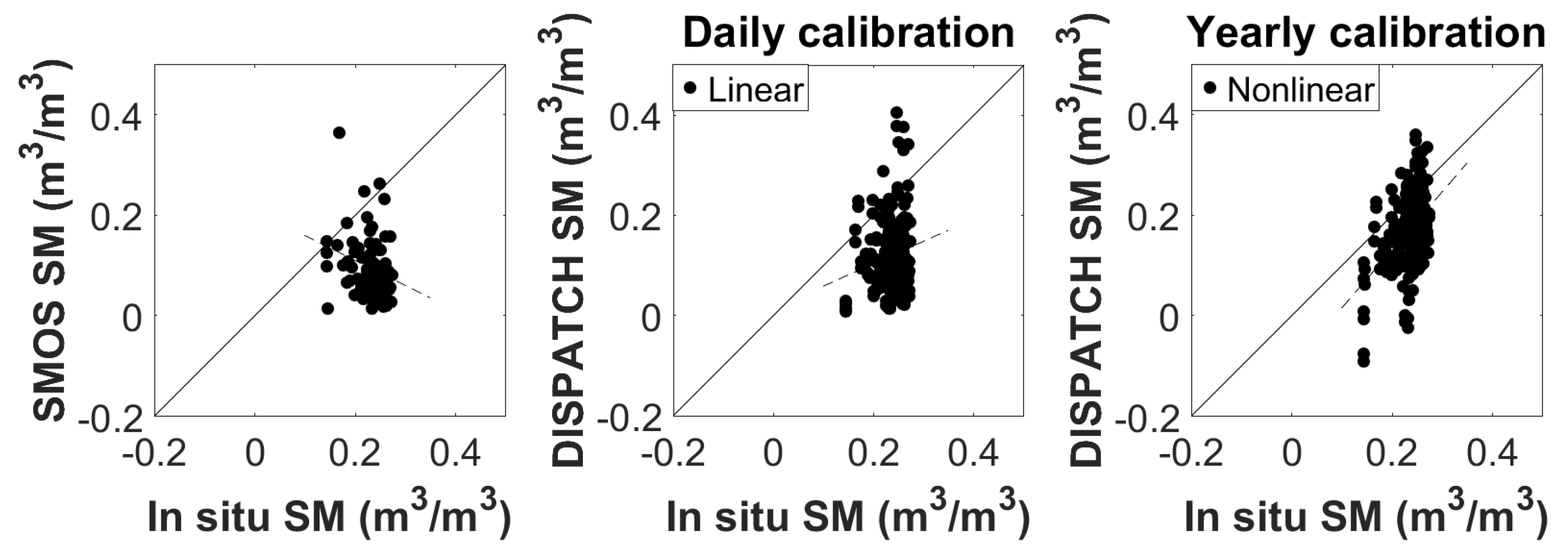
Figure 7,
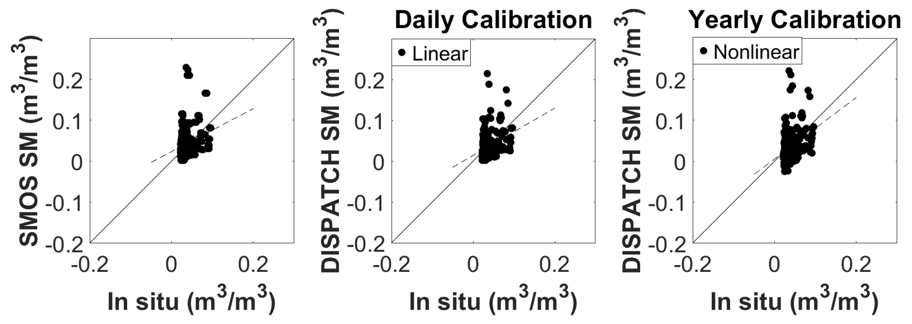
Figure 8 and
Figure 9 show the SMOS SM and the DISPATCH output with respect to in situ measurements for Urgell (2011 and 2015 time periods), Algerri-Balaguer and MOR3. In the same manner as for the spatial validation, the in situ dataset corresponding to Urgell (collected by gravimetric measurements) was aggregated at a 1 km scale by simple linear averaging, for the sampling days. The DISPATCH output presented corresponds to the linear SEE(SM) model with the daily calibration mode, and to the nonlinear SEE(SM) model with the yearly calibration mode.
First, results are presented per calibration mode, and then a discussion will be performed.
4.2.1. Daily Calibration Mode
When analyzing the LR and HR SM values over the areas, DISPATCH improves the fine-scale precision compared to the non-disaggregation case, regardless of the model and calibration. When comparing the linear and the nonlinear models in the daily calibration mode, the nonlinear model performs poorly in the case of Urgell 2015 (corroborating the results obtained for the spatial validation) and Algerri Balaguer.
For Urgell 2011, correlation coefficients equal to 0.27 and to 0.31 (when using the linear and nonlinear modes, respectively) are obtained, as opposed to −0.29 when comparing SMOS SM with in situ data. In a similar manner, for Urgell 2015, the correlation increases from 0.08 (SMOS) to 0.44 (DISPATCH linear mode). In the case of the Algerri-Balaguer site, the correlation coefficient increases from −0.20 (SMOS) to 0.18 (DISPATCH linear mode) and −0.08 (DISPATCH nonlinear mode).
The low correlation values obtained have prompted an analysis (not shown) of the Radio Frequency Interference (RFI) in the SMOS products. Results have shown strong values of RFI in the area of Algerri-Balaguer, which can have an impact on the results. Despite the fact that L3 SMOS SM are RFI filtered [
67], our analysis has shown that RFI effects might remain in the filtered products that we use in our analysis as input to DISPATCH. As for the MOR3 site, the correlation increases from 0.24 (SMOS) to 0.32 and to 0.30 (DISPATCH linear and nonlinear modes, respectively).
The slope of the linear regression is also improved from −0.04 (SMOS) to 0.10 (linear mode) and to 0.13 (nonlinear mode) for the Urgell region, 2011. For 2015, the slope was even further improved, from 0.05 (SMOS) to 0.44 (linear mode). As mentioned in
Section 2, the study areas in 2015 contain two regions in the irrigated area and just one in the non-irrigated one, as opposed to two in 2011. This could possibly explain the better performance in terms of slope obtained, as DISPATCH is well suited to detect well rainfall or irrigation events. In the case of Algerri-Balaguer, the slope has increased from −0.49 (SMOS) to 0.44 (linear mode) and −0.14 (nonlinear mode), respectively. As for MOR3, the slope has increased slightly from 0.52 (SMOS) to 0.58 and 0.61 (linear and nonlinear modes).
In terms of bias, the values remain similar over Urgell, around −0.100 m/m for the 2011 period. For the 2015 period, the bias slightly decreases from −0.079 m/m (SMOS and DISPATCH nonlinear mode) to −0.041 m/m (linear mode). In the case of Algerri-Balaguer, the bias was slightly reduced from −0.138 m/m (SMOS) to −0.114 m/m (linear mode).
As for the Moroccan site, very low bias values have been obtained. This might be explained by the fact that the in situ SM values are very low, as the location of the sensor is close to a desert area. In this area, what SMOS might pick up could be mostly the instrument noise, with a low reported value.
The uRMSE for Urgell 2011 and 2015 report roughly the same value: 0.092–0.102 m/m. For the Algerri-Balaguer region, the uRMSE obtained is roughly around 0.060 m/m in all cases. As for MOR3, very low values are obtained, around 0.030 m/m, for SMOS and DISPATCH linear/nonlinear modes. The low values are explained by the low values of the in situ measurements and of SMOS SM registered over the area.
4.2.2. Yearly Calibration Mode
When comparing the linear and nonlinear models in the yearly calibration mode, the nonlinear model outperforms the linear one. In fact, it gives the best results amongst all model-calibration mode combinations.
Correlations are improved with the nonlinear model to 0.54 for Urgell 2011 and to 0.57 for Urgell 2015. An improvement is also seen for Algerri-Balaguer, obtaining a 0.47 correlation coefficient, as opposed to -0.08 obtained in the linear mode. A similar correlation coefficient as the ones obtained with the daily calibration mode is obtained for MOR3 with the nonlinear model, 0.34.
The highest slope of linear regression, for all sites, is obtained with the nonlinear model: 0.36 (Urgell 2011), 0.47 (Urgell 2015), 1.16 (Algerri-Balaguer) and 0.75 (MOR3), values which are also better than the ones obtained with the daily calibration mode.
In terms of bias, lower values are obtained with the nonlinear model: −0.031 m/m as opposed to −0.079 m/m (Urgell 2015), −0.063 m/m as opposed to −0.153 m/m (Algerri-Balaguer). These values also correspond to the lowest values obtained for the respective sites out of all registered values.
Lower values of uRMSE are obtained by using the nonlinear model, with values remaining roughly between 0.030–0.070 m/m.
Besides its capability of better capturing the nonlinearity effects inherent to the SEE(SM) relationship, the nonlinear model with a multi-date calibration performs better than with the daily calibration mode. This can be attributed to the temporal dynamics of the MODIS-observed SEE used to calibrate the nonlinear model being better suited to characterize the
parameter in Equation (
5). This renders the results more robust, a fact corroborated by the slope of the linear regression systematically improving. In the case of the linear mode, the uncertainties in the retrieved daily
parameter in Equation (
3), which can be partly due to variations in the SEE and/or errors in the SMOS SM, seem to propagate in the multi-date calibration, as
is set to the average of daily
values. Small uncertainties in the model parameterization may have a large impact on the predictions, which could partly explain the poor results obtained with the linear mode with a multi-date calibration. This is not as evident when using the linear model on a daily scale, since there seem to be significant compensation effects between daily SEE and daily
variations.
4.3. General Discussion
Two types of validations have been performed: a spatial validation and a spatio-temporal validation. In terms of spatial validation, DISPATCH clearly captures the spatial variability within the Urgell study area, distinguishing between the dryland and irrigated areas. The nonlinear model with a multi-date calibration systematically performs better than any other. In the case of Urgell 2011, the range of correlation coefficients is improved from [−0.26; 0.49] (nonlinear model, daily calibration) to [−0.23; 0.57]. In the same manner, the higher end of the range of the slope of linear regression is also improved from 0.25 (nonlinear model, daily calibration) to 0.42. In the case of Urgell 2015, the range of the correlation coefficient improves from [0.40; 0.75] (linear model, daily calibration) to [0.57; 0.81].
Looking at the temporal validation, when comparing the daily versus multi-date calibration methodologies, the linear model performs better with the daily mode in the case of Urgell 2015 (corroborating the results obtained for the spatial validation), while the nonlinear model performs better with the multi-date mode. This might be explained by the fact that the nonlinear model is more sensitive to daily changes, while the linear one proves to be more robust. This is consistent with previous studies that have recommended the use of the linear model for DISPATCH applications at 1 km resolution [
15,
18,
48]. In the multi-date mode however, the nonlinear model outperforms the linear model. When comparing the linear and the nonlinear modes, one can conclude that the nonlinear SEE model, with a multi-date calibration, significantly improves the correlation coefficient and the slope of the linear regression, as well as improving (even if slightly), or maintaining, the other statistical parameters. For example, the slope is improved from −0.14 to 1.16 over Algerri-Balaguer, while the correlation coefficient increases from −0.08 to 0.47. The values of the uRMSE are systematically lower, regardless of the study area, when using the nonlinear model with a multi-date calibration. Better results are reported in nonlinear mode with multi-date calibration than in linear mode. In fact, in the nonlinear mode, the partial derivative of SM with respect to SEE is diminished in the lower SM ranges and increased in the higher SM ranges. This entails an overall better precision and accuracy of the corresponding disaggregated products when compared to the in situ measurements. In particular, a small derivative in the lower SM ranges means that the 1 km SM data is approximately equal to the LR SM. In [
18], a comparison has also been made at HR (∼100 m) resolution between the linear model and a different nonlinear model (with a daily calibration), and it was concluded that the nonlinear model is a more adequate choice as it increases the slope of the linear regression between downscaled products and in situ measurements, thus improving the spatial representativeness of SM. The rationale is that the range of SM values within an LR pixel generally increases with the target spatial resolution, and that the nonlinearity effects are more prominent for larger SM spatial variabilities.
An important aspect to mention is the negative values of disaggregated SM when using the nonlinear SEE(SM) model in the downscaling relationship. If we assume that the disaggregation is efficient, then this could point out that SMOS underestimates SM in very dry areas (with SM close to zero). Various calibration and validation studies of SMOS SM products have reported a negative bias [
68,
69,
70,
71]. The bias in the retrieved SM is inflicted by biases in the brightness temperatures, which could be provoked by the RFI for instance. According to [
72], a positive bias in the observed brightness temperature would imply a negative bias in the SM products. Since SMOS SM is used when calibrating the
parameter, the parameter retrieval is also affected by the negative bias. The downscaled SM data obtained in the nonlinear mode is thus affected by both potential biases in the retrieved
values, as well as the negative bias in SMOS data.
It is satisfying to observe that a nonlinear representation of SEE, which is widely acknowledged by a number of in situ and modeling studies, provides systematic better results in terms of SEE-based disaggregation. The key, however, is to develop a calibration strategy adapted to the multi-sensor/multi-resolution data, to their respective uncertainty and to the nature of the model used. Note that the multi-date calibration of each model can be applied over any given period of time, it does not have to be one year only as in our study. However, the multi-date calibration implies a certain latency in the DISPATCH products. In the case of the linear model with a multi-date calibration, the parameter is calibrated as the average of daily values (as previously stated). This implies DISPATCH has to be first run in the daily mode in order to obtain daily values. Similarly, the nonlinear model is calibrated on a muli-date basis using daily data. This also implies DISPATCH has to be first run in daily mode in order to obtain these datasets. Nevertheless, in the case of the nonlinear model, it has been shown that a multi-date calibration proves to be more robust than a daily calibration. Future studies can study the impact of the window considered for the calibration. In fact, choosing a model is also driven by the calibration strategy that can be afforded by this model using the data available at the application scale.
5. Summary and Conclusions
DISPATCH provides 1 km resolution SM data from 40 km resolution SMOS and 1 km resolution MODIS data by combining MODIS-derived SEE estimates at HR and a SEE(SM) model implemented at LR. The SEE model is self-calibrated from MODIS and SMOS data alone. In the current DISPATCH version, the SEE(SM) model is calibrated at a daily scale from quasi-simultaneous MODIS and SMOS observations by assuming a linear SEE representation.
This paper introduces a nonlinear SEE(SM) model in the downscaling relationship. Two calibrations are tested for each SM-based SEE model: on a daily basis and on a multi-date basis.
The approaches are tested by comparing the disaggregated SM values with in situ measurements over two mixed dry and irrigated areas in Catalonia (Spain)—spanning 2011 and 2015 (Urgell area) and 2017–2018 (Algerri-Balaguer), and over a dry area in Morocco (MOR3) in 2016–2017. Two types of validations are performed: a spatial validation and a spatio-temporal validation.
When comparing the two models in the daily calibration mode (both for the temporal as well as the spatial validation), the linear model gives better results in the case of Urgell 2015, improving the slope of linear regression, correlation coefficient and bias values. The correlation coefficient is equal to 0.44 (temporal validation), while the slope of the linear regression is increased to 0.44 (temporal validation).
The integration of a nonlinear SEE(SM) model with a multi-date calibration systematically improves the statistics over all sites (for both the spatial and the temporal validation). The temporal correlation is increased to 0.57 and 0.47 for Urgell 2015 and Algerri-Balaguer, while the slope of linear regression is 0.47 and 1.16, respectively. The introduction of a nonlinear model with multi-date calibration systematically lowers the values of the uRMSE, regardless of the study area.
The low correlations obtained over all Spanish sites could also partly be explained by some small RFI (Radio Frequency Interference) sources detected within the area. An analysis of the SMOS products was performed over the Spanish sites and it has shown high values of RFI. This leads to erroneous measurements by SMOS, which propagates in the downscaled products, regardless of the SM-based SEE model and of the calibration used.
Keeping in mind that the calibration strategy is to be adapted to the multi-sensor/multi-resolution data and to the SEE(SM) model used, the nonlinear SEE(SM) model has proven to perform significantly better under various conditions, with more robust disaggregated SM products being obtained.
The SEE modeling based on the nonlinear SM model, with a multi-date calibration, could be integrated into the CATDS—Centre Aval de Traitement des Données SMOS [
15] as a future new product, into existing evapotranspiration models, which are based on a combination of thermal and microwave data [
73,
74], as well as into a new stepwise disaggregation approach using DISPATCH at an intermediate spatial resolution [
65].

 ,
, 


