Article

Geographic Object-Based Image Analysis Framework for Mapping Vegetation Physiognomic Types at Fine Scales in Neotropical Savannas

by
Fernanda F. Ribeiro
1,*,
Dar A. Roberts
1,
Laura L. Hess
2,
Frank W. Davis
3,
Kelly K. Caylor
1,3 and
Gabriel Antunes Daldegan
1
1
Department of Geography, University of California, Santa Barbara, CA 93106, USA
2
Earth Research Institute, University of California, Santa Barbara, CA 93106, USA
3
Bren School of Environmental Science and Management, University of California, Santa Barbara, CA 93106, USA
*
Author to whom correspondence should be addressed.
Remote Sens. 2020, 12(11), 1721; https://doi.org/10.3390/rs12111721
Submission received: 27 April 2020 / Revised: 25 May 2020 / Accepted: 25 May 2020 / Published: 27 May 2020

Abstract

:
Regional maps of vegetation structure are necessary for delineating species habitats and for supporting conservation and ecological analyses. A systematic approach that can discriminate a wide range of meaningful and detailed vegetation classes is still lacking for neotropical savannas. Detailed vegetation mapping of savannas is challenged by seasonal vegetation dynamics and substantial heterogeneity in vegetation structure and composition, but fine spatial resolution imagery (<10 m) can improve map accuracy in these heterogeneous landscapes. Traditional pixel-based classification methods have proven problematic for fine spatial resolution data due to increased within-class spectral variability. Geographic Object-Based Image Analysis (GEOBIA) is a robust alternative method to overcome these issues. We developed a systematic GEOBIA framework accounting for both spectral and spatial features to map Cerrado structural types at 5-m resolution. This two-step framework begins with image segmentation and a Random Forest land cover classification based on spectral information, followed by spatial contextual and topological rules developed in a systematic manner in a GEOBIA knowledge-based approach. Spatial rules were defined a priori based on descriptions of environmental characteristics of 11 different physiognomic types and their relationships to edaphic conditions represented by stream networks (hydrography), topography, and substrate. The Random Forest land cover classification resulted in 10 land cover classes with 84.4% overall map accuracy and was able to map 7 of the 11 vegetation classes. The second step resulted in mapping 13 classes with 87.6% overall accuracy, of which all 11 vegetation classes were identified. Our results demonstrate that 5-m spatial resolution imagery is adequate for mapping land cover types of savanna structural elements. The GEOBIA framework, however, is essential for refining land cover categories to ecological classes (physiognomic types), leading to a higher number of vegetation classes while improving overall accuracy.

Graphical Abstract

1. Introduction

Monitoring patterns and trends in tropical savannas still faces major uncertainties related to their definition and classification [1,2,3,4]. This uncertainty is reflected both in general land cover classification and maps featuring vegetation physiognomic types (e.g., life form, vegetation cover). For example, savannas are poorly defined in global land cover products, and variation in their physiognomic types is not well classified at local scales [2,5,6]. Most current technology featuring moderate to coarse spatial resolution (>10 m) fails to resolve the fine-scale heterogeneity of savannas. Major issues in their discrimination relate to growth patterns (associated with seasonality of contrasting dry and wet seasons) and to admixtures of life forms and land cover categories at operational sensor scales [7,8].
Savannas occupy a significant area of the tropics, covering approximately 20% of the world’s land surface [3,9]. Tropical savannas, for example the Argentinian Chaco, the African Miombo, and the Brazilian Cerrado, are often intermixed with riparian forests, swamps, and marshes [9]. They are composed of a herbaceous stratum in a discontinuous tree and shrub cover of varying height and density [2,3,10]. The Cerrado, a neotropical savanna in Brazil, is the most floristically diverse savanna in the world, with more than 12,000 plant species [11], including numerous endemics [12,13]. Moreover, the Cerrado provides critical ecosystem services such as carbon storage [14] and plays a major role in provision of water resources by hosting the headwaters of the three largest watersheds in South America.
Land cover mapping of savannas has been conducted mostly at regional scales, using optical sensors available at moderate (10–500 m) to coarse (>500 m) spatial resolution, such as the Landsat series and Moderate Resolution Imaging Spectrometer (MODIS). Most studies focus on multi-temporal analysis for change detection [15,16,17,18], deforestation monitoring [19,20,21,22], and land surface phenology [23,24,25]. Specific challenges to savanna land cover classification are related to: (a) high sensitivity to sensor resolution due to discontinuous tree canopy cover [26]; (b) high seasonal variation in ecosystem properties, cloud cover, and data availability [27]; and (c) smoke and haze due to frequent fires in the dry season [28].
As for other savannas, discriminating spectrally similar shrubs from trees with moderate-to-coarse resolution imagery has proven challenging for the Brazilian Cerrado [23,29]. Sano et al. [30] used image segmentation and visual interpretation of Landsat to produce a map of natural and converted areas for the entire Cerrado region. Other Landsat-based studies have focused on local sites to investigate methods for mapping fractional woody cover, such as spectral unmixing [29], and Support Vector Machine classification of multi-year phenologic profiles based on the Tasseled Cap Transform [25]. Several studies took advantage of multi-temporal rather than single-date imagery to overcome spectral similarities in woody cover using characteristic phenological patterns [17,23,25,31,32]. Although these approaches are useful for broad-scale analyses, they depict coarse structural vegetation classes [25,33,34,35] and cannot resolve the structural heterogeneity essential for regional biodiversity and ecosystem assessments [36].
A critical problem in mapping Cerrado physiognomic types concerns the definition of classes. Most previous remote sensing studies considered a widely adopted vegetation nomenclature for the Cerrado physiognomies based on structural attributes and floristic composition (see Ribeiro and Walter [37]). Vegetation maps exhibiting the diverse structural variation in vegetation types are critical for representing fine-scale savanna habitat patterns. Spectrally based remote sensing analyses based on floristic classification systems (such as Ribeiro and Walter [37]) may not succeed in identifying structural differences in vegetation and may require extensive field work for species identification. Thus, they may not be suitable for regional scale mapping using multispectral imagery classification alone. Geographical characteristics related to edaphic conditions (e.g., topography, soils), however, can potentially help identify some physiognomic types not strictly based on species composition.
Remote sensing imagery at fine (<10 m) spatial resolution can better capture the diversity in vegetation structure of heterogeneous and complex savanna landscapes [36,38,39,40,41]. However, traditional pixel-based classification methods have proven problematic for fine spatial resolution data due to increased within-class spectral variability, potentially leading to inconsistent results [42,43]. Geographic Object-Based Image Analysis (GEOBIA) bridges remote sensing and Geographic Information Science by defining image objects as entities and focusing on the conceptual modeling of defined land cover classes at multi-scales. Thus, GEOBIA is a robust alternative approach to address within-class spectral variability issues in land cover classification of high spatial resolution imagery and heterogeneous landscapes [42].
GEOBIA is based on extracting information from Earth Observations using spectral, spatial, structural, and hierarchical properties of an image [44]. A fundamental step is to delineate objects of interest, which are strongly associated with image segmentation approaches that cluster relatively homogenous pixels into image objects. One of the significant advantages of the GEOBIA approach is that image objects provide not only diverse spectral information (e.g., mean values per band, standard deviation, mean ratios) but also additional spatial information, such as distance, neighborhood, and topological metrics [42,45]. The combination of spectral and spatial properties allows incorporation of contextual information of a given object using ontologies/semantics to create hierarchical conditional rules tailored to classify meaningful object definitions in a knowledge-based classification [42,46].
Efforts to map fine-scale structural variation in savanna ecosystems using GEOBIA have obtained encouraging results compared to moderate spatial resolution data and pixel-based methods [26,39,41,47,48]. GEOBIA is also increasingly used for Cerrado studies due to the recent availability of fine (5 m) spatial resolution imagery from the RapidEye sensor at no cost for Brazilian researchers. Initial efforts to evaluate the utility of high spatial resolution imagery for discriminating and mapping Cerrado physiognomic types have demonstrated improved discrimination of structural classes and higher map accuracy compared to coarser resolution imagery [49,50,51]. Such efforts include using supervised object-based classification with several input object features in a GEOBIA context, such as in Girolamo-Neto [49] and Girolamo-Neto et al. [41]; or strict knowledge-based classification by defining conditional rules based on shape and brightness parameters, such as in Teixeira et al. [51]. However, these studies were tested at sites with limited extent (< 50,000 ha) such as Brasilia National Park, which does not include some major vegetation structural types known for causing misclassification errors (i.e., semi-deciduous versus deciduous forest [51]), or featured coarse vegetation classes as opposed to detailed physiognomic types. A systematic approach that can discriminate a wide range of meaningful and detailed vegetation classes is still lacking for the Cerrado biome.
The primary goal of this study is to develop a systematic framework to discriminate detailed Cerrado physiognomic types in a semi-automatic manner using single-date high spatial resolution imagery. The rationale for mapping detailed physiognomic types at fine scales stems from the potential of such maps to (1) improve our understanding of species habitat requirements and conditions, as well as our ability to assess ecosystem services and biodiversity [36], and (2) provide improved inputs for fire modeling, carbon accounting [52], landscape restoration [53], and land-use management [54]. Our approach takes advantage of GEOBIA and semantics to combine land cover classes and edaphic conditional drivers in the definition of hierarchical contextual rules used to classify a wide range of Cerrado physiognomic types. The specific research questions we aim to answer with this framework are: What accuracies are achievable using spectral information alone? What accuracies are achievable adding spatial context information? How can the widely adopted Cerrado physiognomic types nomenclature be used in a remote sensing analysis? We address these questions using RapidEye imagery (5 m) in a two-step GEOBIA framework that begins with a supervised object-based land cover classification based on spectral information alone, followed by assignment of spectral land cover classes to more detailed physiognomic types using a novel hierarchical spatial and topological ruleset defined by semantics (i.e., descriptive assessment and knowledge). This approach takes advantage of ancillary information on hydrography, topography, and substrate as environmental conditional drivers in the semantic definition of hierarchical contextual rules. This GEOBIA framework was tested for two large study sites covering most major Cerrado physiognomic types. Its main advantages relate to its reproducibility across different areas of this heterogeneous biome, its capacity to discriminate a wide variety of physiognomic types that could not be distinguished in previous studies, and its adaptability to other physiognomic types and to other types of optical imagery.

2. Materials and Methods

2.1. Study Sites

The Cerrado has a tropical climate characterized by an October–April wet season and May–September dry season, when rainfall can be close to zero [55]. Plant distributions across the Cerrado are mostly determined by topography, soil texture, nutrient content and depth, fire regime, and water availability [56,57]. Spatial variation in these environmental conditions results in high beta diversity across the biome as well as large variability of physiognomic types over relatively small distances [37,58].
We chose two study sites (Figure 1) to test our classification framework and compare its accuracy in discriminating savanna vegetation with differing landscape composition and surface heterogeneity. The sites were chosen based on their ecological importance for conservation, their differences in composition and beta diversity, and a combination of imagery and ancillary data availability.

2.1.1. Study Site 1: Taquara Watershed

We initially tested our method at the Taquara site (Figure 1), a study site for which we had high-quality orthophotos (24 cm resolution) and a greater availability of ground reference and ancillary data that were important for testing our ability to visually identify physiognomic types using air photos when collecting training data. The Taquara site (15°54′S, 47°55′W to 15°58′S, 47°50′W) comprises an area of 67.3 km2 located approximately 26 km from downtown Brasília, covering most of the Taquara watershed and its surroundings. This site also contains the Brazilian Institute of Geography and Statistics (IBGE) Ecological Reserve, a protected area created to act as a biodiversity control site for comparison to other Cerrado areas altered by human occupation. The IBGE Ecological Reserve served as one of the Cerrado sites included in the Large Scale Biosphere-Atmosphere Experiment in Amazonia (LBA) [59], and was the first International Long Term Ecological Research (ILTER) site in the Cerrado biome.
The watershed is located in the Cenozoic bed from the Paranoa Group and terrain is relatively flat, with elevation in the region varying between 1040 and 1196 m. Mean annual precipitation is 1426 mm and mean annual temperature is 23 °C [60]. The site has considerable diversity of plants and soil types, representing most of the typical physiognomic types found across the Cerrado. Soils are mostly acidic, low fertility Oxisols (Latosols) supporting savanna ecosystems. Organic, nutrient-rich hydromorphic soils occur locally in the area and often support forest ecosystems. Most of the site is covered by savanna ecosystems, but grasslands located on small hills, and gallery forests with surrounding wetlands following small streams are also present. Common tree species include Pterodon pubescens, Bowdichia virgilioides, Vochysia thyrsoidea, and Dalbergia miscolobium, while grasses are dominated by perennial species such as Echinolaena inflexa, Schizachyrium tenerum, Trachypogon spicatus, and Axonopus chrysoblepharis [61].

2.1.2. Study Site 2: Western Bahia

We also tested whether our method could be applied to a larger and even more heterogeneous site with minimal ground reference and ancillary data. This study site comprises an area of 9409 km2 and is located on the western side (11°43′S, 45°52′W to 12°36′S, 44°59′W) of the São Francisco River watershed, the largest river basin entirely located in Brazilian territory (Figure 1). The Western Bahia site is not only naturally heterogeneous but also has considerable complexity due to historical land use conversion of natural savanna to pasture and row crop agriculture [18]. Elevation ranges from a maximum of 808 m across karstic mesas/plateaus (known as Chapadões do São Francisco) to 433 m in the lowest point in the São Francisco Depression, with annual precipitation ranging from 800 mm at lower elevations to 1600 mm at highest elevations [54,62]. The plateaus are composed of Proterozoic rocks from the Bambui Group and Cretaceous beds from the Urucuia Group. Diverse soils include deep well-drained Oxisols (Latosols) of medium texture in the highest parts of the plateau and sandy texture (sandy quartz) on irregular terrain, rocky soils (Lithosols) of sandy to medium texture on steep slopes and escarpments, and hydromorphic/organic soils across floodplains [62]. This variety of edaphic conditions supports diverse vegetation types mostly consisting of savanna ecosystems across the plateaus, wetlands and riparian vegetation along floodplains, and semi-deciduous forest restricted to cliffs and to the eastern part of the plateau, which is possibly due to local concentrations of calcium carbonate in the soil and higher moisture conditions [62]. In general, lower elevation sites have greater physiognomic diversity compared to the plateaus [63].
Common tree species within the savanna ecosystem include Anacardium occidentale and Miconia ferruginea, and the grass layer is dominated by annual species such as Ichnantus hoffmannseggii [64]. Seasonally dry tropical forests are mostly found along escarpment slopes, and are composed of deciduous or semideciduous tree species such as Astronium urundeuva, Piptadenia macrocarpa, Chorisia speciosa, Tabebuia spp., Cavanillesia arborea, and Cedrella fissilis [65].

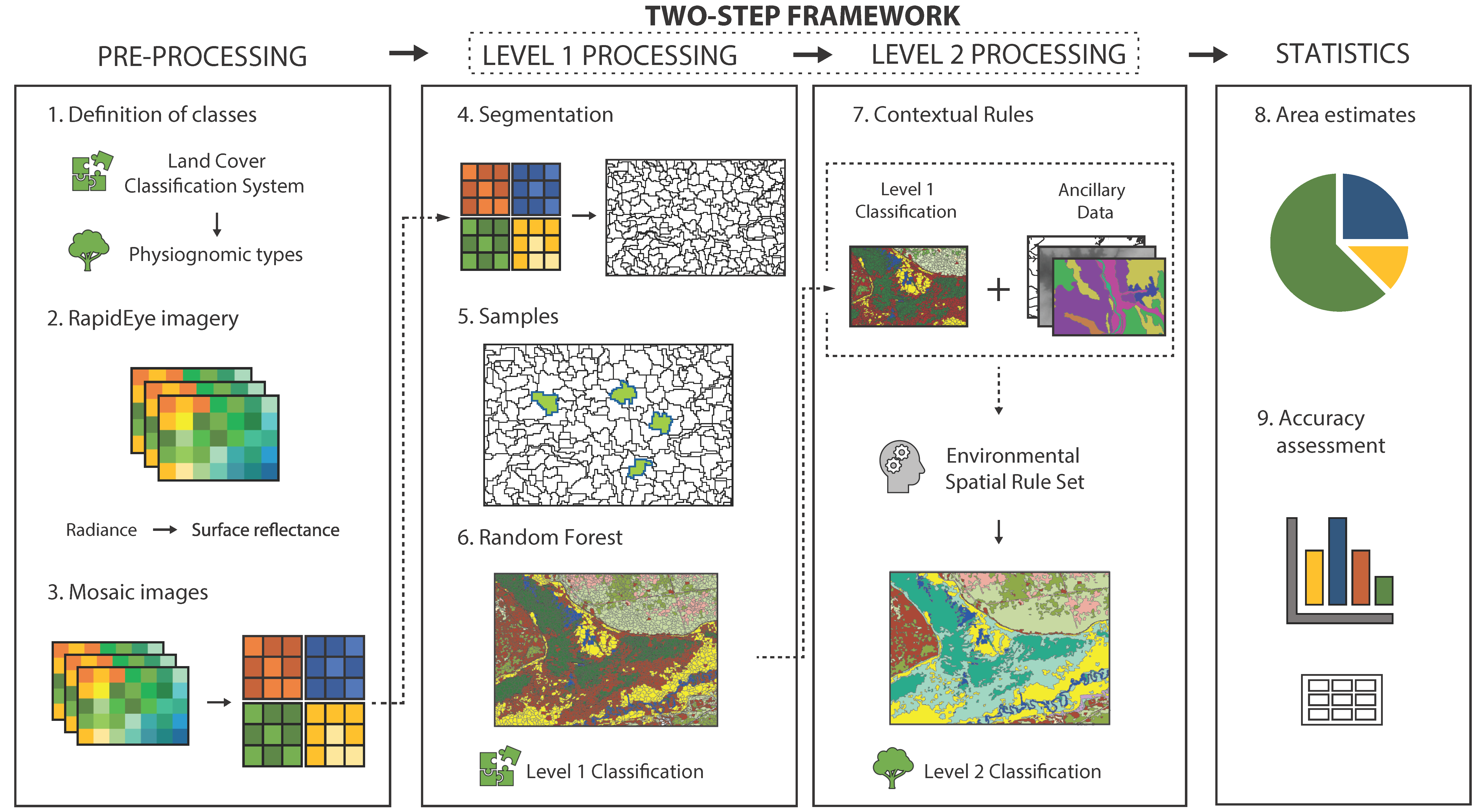
2.2. Methods Overview

The GEOBIA framework used in this study is divided into two major steps (Levels 1 and 2), in addition to pre and post-processing stages: (a) pre-processing; (b) land cover classification (Level 1 processing); (c) physiognomic types classification (Level 2 processing); (d) area estimates; and accuracy assessment (statistics). These procedures are shown and described in detail in Figure 2.

2.2.1. Definition of Classes

The Cerrado physiognomic types have been defined by many authors such as Coutinho [66], Eiten [67], and Oliveira-Filho and Ratter [57]. The most recent vegetation terminology proposed by Ribeiro and Walter [37] has been widely adopted by the scientific community in Brazil. This scheme, however, is based on criteria such as environmental edaphic conditions and species composition that are not reliably detected by multispectral sensors. Thus, translating these on-the-ground Cerrado classification schemes to a land cover classification derived from remote sensing is a challenging task.
The United Nations Food and Agriculture Organization’s (FAO) Land Cover Classification System (LCCS) is a flexible and systematic framework designed for land cover classification terminology at any given scale and for any data source [68]. The LCCS framework defines classes at different levels, starting with broad distinctions (e.g., Primarily Vegetated Areas, Primarily Non-Vegetated Area) within a dichotomous key and then adds specific attributes through a hierarchical framework (e.g., life form, cover, height). Classes are then defined as a function of the intended level of detail (scale) for the land cover classification based on a combination of the spatial and spectral resolution of the imagery, which makes the LCCS appropriate for object-based classification [69].
To allow for standardization among Cerrado classes, we used the LCCS as a reference in the first classification level. The classes were defined a priori, based on a literature review of major physiognomic types found across the Cerrado. In accordance with the RapidEye spatial and spectral characteristics, the quality of the images (e.g., off-nadir viewing angles), and the recommended scale for mapping Cerrado physiognomic types [37], the map scale was defined as 1:25,000. We followed the LCCS criteria based on dominant life form, vegetation cover, and structure, as well as water seasonality (Figure 3). In the second classification level (Figure 3), we followed the nomenclature described by Ribeiro and Walter [37] for our map legend of physiognomic types (Table 1).

2.2.2. Imagery Acquisition and Pre-Processing

Most RapidEye imagery used in this study was acquired in the 2011 dry season, representing the imagery with the best quality available. The commercial RapidEye sensor, launched in 2009, operates in a constellation of five satellites in the same orbit, providing multispectral images with a spatial resolution of 6.5 m resampled to a 5-m grid (at the Level 3A), and a tile size of 25 km by 25 km. The sensor has a swath width of 77 km, daily off-nadir coverage, and radiometric resolution of 12 bits, scaled up to a 16-bit dynamic range. RapidEye’s spectral resolution covers the visible and near-infrared bands ranging from 440 to 850 nm, including a red-edge band (690 to 730 nm). The imagery is available through the Ministry of Environment (MMA) Geocatalog and is accessible to Brazilian researchers at no cost. The collection covers the entire country and is composed of varying off-nadir angles and temporal coverage, which is limited to inconsistent dates mostly available for the years 2011 through 2015, depending on the area of interest.
Although the orthorectified Level 3A RapidEye product is provided with radiometric, geometric, and terrain corrections, additional corrections were made for improving consistency in the product. Atmospheric corrections and reflectance retrieval were performed using ACORN 4.0 software for all individual imagery tiles. Calibration files corresponding to image spectral response, gain, and offset, as well as acquisition parameters, were created from the metadata provided. Water vapor and atmospheric visibility parameters were determined by a trial-and-error analysis of a dark object reflectance (e.g., pure water pixels) and following the ACORN user guide suggestions for areas of dry conditions.
In total, we used 17 RapidEye imagery tiles. One tile corresponds to most of the Taquara watershed, covering the IBGE Ecological Reserve and its surroundings (Figure 1). After applying the atmospheric correction and reflectance retrieval, the image was subset to the bounding box extent of the watershed to facilitate data processing. The other 16 images correspond to the Western Bahia study site (Figure 1). The pre-processing steps were applied to individual imagery tiles, and tiles with the same acquisition date were mosaicked. The individual mosaics were processed separately, at both classification levels, and merged together to derive statistics for the complete study site (i.e., accuracy assessment and landscape composition). The Taquara tile was acquired on August 11th 2013, and the Western Bahia tiles were acquired from June to October 2011. Details of imagery tiles, dates, and sensor angle-viewing characteristics are summarized in Table S1.

2.2.3. Level 1 Classification: Major Land Cover Types

(1) Segmentation
Our GEOBIA approach starts with segmenting the images into homogeneous image objects to ensure neighboring pixel similarity at an adequate scale. The segmentation was performed through the multi-resolution segmentation (MRS) algorithm, proposed by Baatz and Schäpe [70] and implemented in eCognition Developer 8.0 software. For all images, the segmentation used all five spectral bands of the RapidEye image, with higher weights for near-infrared (NIR) (760–850 nm), red-edge (690–730 nm), and red (630–685 nm) bands due to their importance in discriminating vegetation types [23,71]. The multi-resolution algorithm implemented in eCognition uses a bottom–up merging approach as an optimization procedure to identify similar, homogenous, neighboring pixels and cluster them into a single object. eCognition accounts for a scale parameter as a level of aggregation of image objects and uses a stop criterion in the optimization algorithm. Thus, the scale is a crucial part of GEOBIA, as it defines the size of image objects as well as their level of heterogeneity. The multi-resolution algorithm also accounts for shape and compactness parameters. We visually inspected multiple combinations of scale, shape, and compactness parameters and selected a combination of scale = 10, shape = 0.3, and compactness = 0.7. These parameters are in accordance with other GEOBIA studies that use high spatial resolution imagery and have small image object scale [72].
(2) Collection of training data and Random Forest model
The training data were collected through a process of visual interpretation assisted by orthophotos and Google Earth images covering both study sites. We defined standard parameters for visual interpretation of the classes, which were assisted by ancillary data (such as other vegetation maps available for the sites) and one field excursion conducted in the dry season of 2018 to each site for confirmation of class categories in areas that were still unclear after examining the available resources.
Training samples were collected in proportion to class abundance, with abundant classes having a higher number of training data compared to classes that were rare across the landscape (Table S2). All training was done at the object scale, in which each sample corresponds to an image object generated in the segmentation process. Spectral variables (e.g., statistics and indices), also known as object features in GEOBIA, were attributed to each training polygon (Table 2), including three indices: Normalized Difference Vegetation Index—NDVI [73], Normalized Difference Vegetation Index with red-edge band—NDVI-RE [71], and Normalized Difference Water Index—NDWI [74].
All training samples and their respective statistical attributes were used as input in the ‘random forest’ package in RStudio developed by Liaw and Wiener [75] based on Breiman [76]. All parameters were set to default on the random forest classification algorithm, which resulted in a model based on 500 decision trees used to classify all image objects derived from the multi-resolution segmentation. The result of this process is the Level 1 land cover classification based on the LCCS land cover classes.

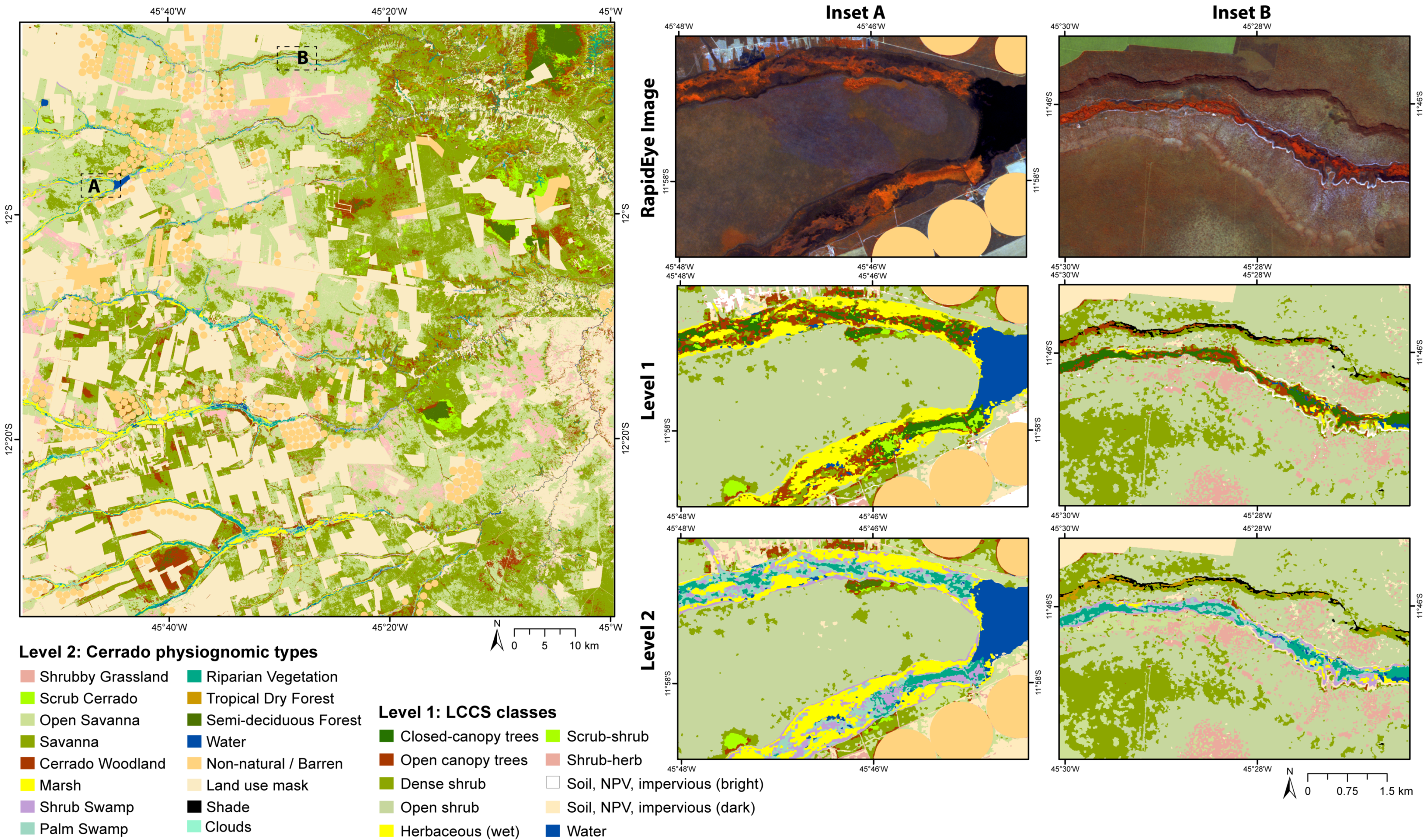
2.2.4. Level 2 Classification: Physiognomic Types

In accordance with our goal of classifying physiognomic types in a semi-automatic manner, we developed a series of spatial contextual rules for each study site in order to refine the Level 1 land cover map (Table 3). We combined the Level 1 LCCS classification with hydrographic data (stream networks and hydromorphic soils) developed by Ribeiro [77] for the Taquara site (scale 1:10,000); and by the Laboratory of Spatial Information Systems–LSIE at the University of Brasília (Brazil), in partnership with the Inter-American Institute of Commerce and Agriculture and the Brazilian Ministry of National Integration, for the Western Bahia site (scale 1:2000). Slope and elevation were derived from the NASA Digital Elevation Model–NASADEM [78] available at a resolution of 1 arc-sec (approximately 30 m).
The spatial rules were developed based on environmental characteristics of the vegetation physiognomic types described in Pereira and Furtado [61], Nou and Costa [62], and Ribeiro and Walter [37], in addition to personal and expert knowledge of the study sites. Specific elevation and slope thresholds were based on recommendations from the Brazilian Agricultural Research Corporation–Embrapa [79]. The same contextual and topological rules were applied for both study sites, except that thresholds used for elevation and slope were adapted to each site’s characteristics.
The combination of mountainous terrain (e.g., escarpments/cliffs) and fine spatial resolution resulted in a high presence of shadows in the Western Bahia site imagery. However, RapidEye’s spectral resolution does not allow us to distinguish shadows from water, a well-known source of confusion in remote sensing and multispectral high resolution images [35]. We therefore developed a “shade” mask using a topological rule in eCognition. We also used visual interpretation to create a “cloud” and “shade from cloud” mask, and a “water body” mask was created for the Taquara site, given that this class was rare and small enough (<0.01%) to not be included in the model. Because we were exclusively interested in natural areas, a land use mask from our database (data from [18,77]) was used in each study site to exclude paved roads, agricultural, and urban areas from validation.

2.2.5. Accuracy Assessment Procedures

Measuring thematic map accuracy is a crucial step to determine error sources and calculate producer and user map accuracies. Moreover, it is a way to analyze potential weakness and strengths of classification methods. However, it is not a straightforward task and can include many uncertainties [80, 81,82,83,84]. In traditional pixel-based classification, thematic accuracy is assessed by estimating the proportion of correctly classified pixels for each class. This approach assumes that pixels have the same size, and thus, one can estimate the proportion of area correctly classified [83]. However, it is recommended that image objects are used as sampling units in object-based accuracy assessments, instead of the traditional point-sampling from pixel-based classification [85]. Image objects have variable areas across the landscape in GEOBIA-derived thematic maps, leading to a greater impact on error estimates from large misclassified objects than small polygons. Thus, area count should be accounted for in accuracy assessments of GEOBIA classification [86].
The Random Forest algorithm generates an out-of-bag (OOB) error estimate using subsampling and bootstrapping, accounting for samples not used as training in the model [76]. To minimize inflated accuracies from the OOB error due to spatial autocorrelation, we performed additional independent validation for both study sites. This independent validation was done by comparing randomly selected polygons from our classified images (excluding training samples) to a series of ancillary data, including orthophotos, Google Earth imagery, and digital photographs (taken on the ground), when available, following recommendations from Richards [83]. Given the lack of fine-scale time series imagery available for the entire landscape, experts with local knowledge of the sites were also consulted to validate the classes that are influenced by seasonality. For instance, the natural seasonality of seasonally dry tropical forest and semi-deciduous forest required local knowledge when the time series of Google Earth imagery was not available. We performed the sampling selection using the original segments/objects derived from eCognition, which contain information at both map levels. The number of samples for each category was determined based on the final map (physiognomic types), but accuracy estimates were performed for both levels using the same polygon. We used an equal proportion of randomly selected polygons for categories that were sparsely represented across the landscape (≤10%), which resulted in a total of 50 polygons per class. For classes with high landscape abundance (i.e., non-natural/barren, open savanna, savanna for both sites), we performed a stratified random selection based on a total number of samples of 225 for each site. The classes “semi-deciduous forest” and “shrub swamp” were not accounted for in the validation process for the Taquara site because they each represent less than 0.5% of the landscape. In total, we selected 725 polygons for the Western Bahia site and 525 polygons for the Taquara study site.
A common issue in estimating accuracy from thematic maps is the potential error that can be included in the reference data [81,82,87]. To minimize error and bias from the interpreter in the accuracy assessment, our validation procedures were performed by two authors trained in photointerpretation of the regions and with previous experience working in the Cerrado. Error matrices were generated for each map level using an area-weighted approach based on independent sampled image objects [69,86]. The traditional count-based accuracy assessment was also performed for comparison (Tables S5–S8). They were used to derive traditional statistical accuracy measures for both map levels, such as overall agreement, user’s accuracy, and producer’s accuracy.

3. Results

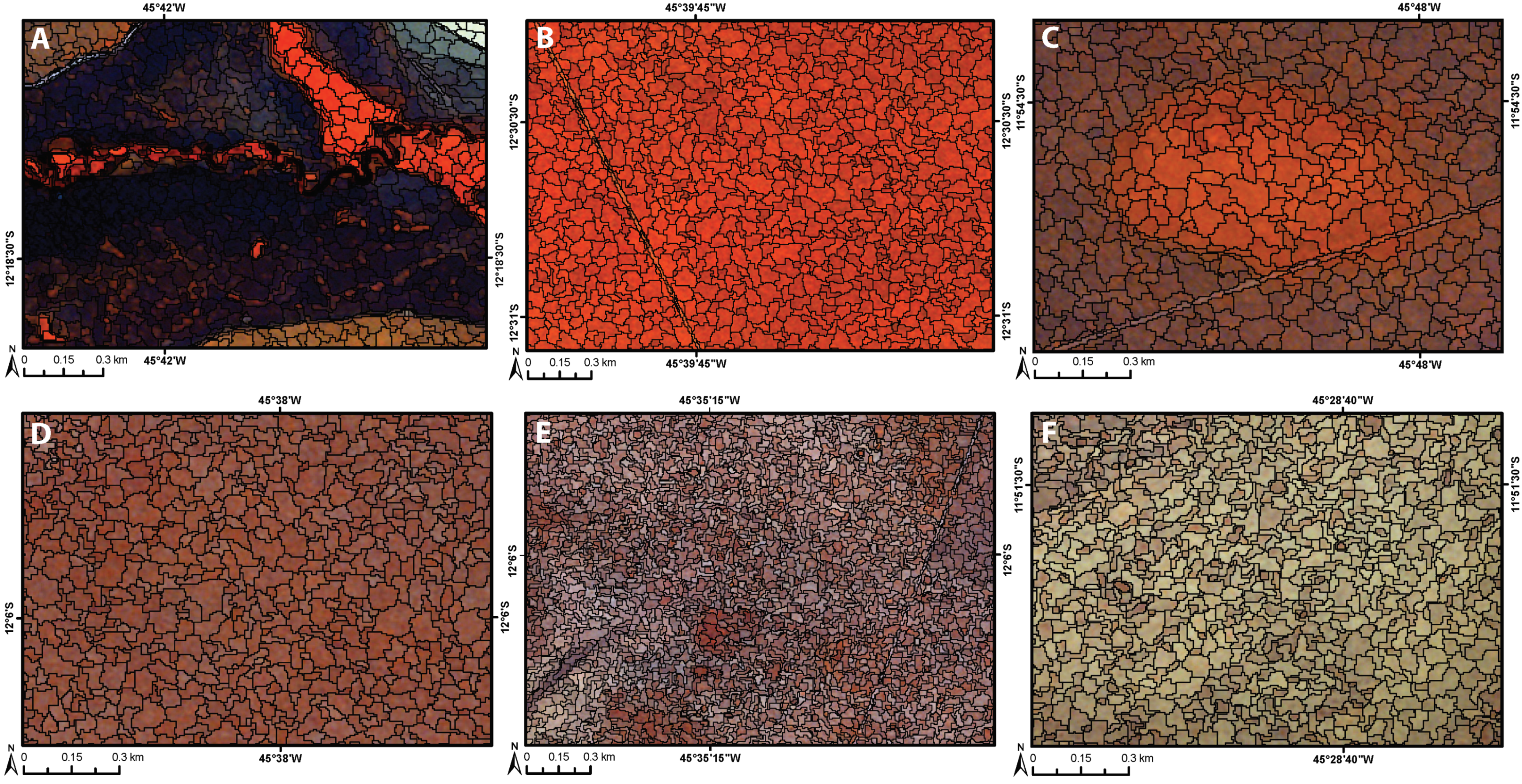
3.1. Segmentation Results

The MRS algorithm generated a different number of image objects (Figure 4) for each mosaic or image tile processed, which is expected since they have different extents. The imagery tiles acquired in September 16th and September 13th resulted in 384,011 and 389,664 objects, respectively. The August and October mosaics have similar extent (4 image tiles) and resulted in 1,157,419 and 979,083 objects, respectively. The June mosaic contains 6 image tiles and thus resulted in a much larger number of objects, a total of 2,804,338.

3.2. Accuracy Assessment

The OOB error for the Taquara site was 7.8%. Given that the Random Forest classification was performed by mosaic for the Western Bahia site, the OOB error estimates were then generated for each mosaic. The September 13th image had the lowest OOB error (3.5%). The October mosaic had the second lowest OOB error (4.4%), followed by the September 16th imagery (6.3%), the August mosaic (7.0%), and the June mosaic (7.3%).
These relatively small differences in the OOB error estimates could be due to a combination of reasons such as atmospheric conditions on a particular day (e.g., active fire was present in the June mosaic, and haze was present in the September 16th imagery), possible rain close to the imagery date, differences in sensor angle-viewing, and particular characteristics of the classified image (e.g., one specific image can have more disturbed areas and hold higher heterogeneity compared to the other).
The mean decrease in accuracy is a percent estimate of variable importance in the random forest model (Figure 5). The NDVI was the most important variable in all models, except in the June mosaic, in which NDWI had the highest importance. This is likely due to water content available in the soil during early dry season (i.e., June), whereas later in the dry season, some physiognomies (i.e., grass and shrublands) are more impacted by water limitation. The other indices, NDVI (red-edge) and NDWI, also contributed significantly (>12%) in all models. Considering only the RapidEye spectral bands, the near-infrared (band 5) had a contribution above 13% in all models, whereas the red and red-edge bands had high importance (>15%) in the October and June mosaic models, respectively.
Additional accuracy estimates based on the independent randomly selected image objects were performed for the entire map and not for individual mosaics. Error matrices were developed for each map level (Table 4 and Table 5) and were reported as area (in hectares) count of each image object, following best practices for object-based accuracy assessment proposed by Radoux et al. [69]. Statistical measures of overall agreement, as well as user’s and producer’s estimates were derived from the error matrices (Table 4 and Table 5). For comparison, we also generated error matrices and statistical measures based on the regular polygon count approach (Tables S5–S8). Accuracy assessments for the Taquara watershed are found in the supplementary material (Tables S3–S4).

3.3. Landscape Composition: Area Assessments

We estimated landscape composition (Table 6) for the total area of the Western Bahia site, as well as for each mosaic, based on the final (Level 2) physiognomic type map (Figure 6). The most abundant classes in the landscape are non-natural/barren areas, open savanna, and savanna. The rarest physiognomic types found are seasonally dry tropical forest, shrub swamp, and palm swamp. Considering the individual mosaics, the June mosaic and the September 13th image have the highest amount of natural vegetation, whereas the October mosaic has the highest concentration of non-natural/barren areas. The Level 2 classification map and landscape composition of the Taquara watershed is found in the supplementary material (Figure S1, Table S9).

4. Discussion

Land cover mapping in the Cerrado has generally used multispectral imagery with medium to coarse spatial resolution and pixel-based approaches, such as in Muller et al. [17], Schwieder et al., [25], Ferreira et al. [29], and Reynolds et al. [88]. As demonstrated by Sano et al. [30] and Schwieder et al. [25], these types of imagery do not capture the fine-scale heterogeneity present within the savanna ecosystem gradient and thus are not appropriate to discriminate differences in vegetation structure, often leading to low accuracy results (such as 71% and 63%, respectively). Distinguishing the fine-scale heterogeneity of Cerrado physiognomic types is crucial for identifying species habitats and estimating plant diversity. For instance, the Hyacinth Macaw (Anodorhynchus hyacinthinus) is an endangered species of small population inhabiting the Cerrado that is heavily dependent on palm trees present in wetlands for breeding and foraging; discriminating the different structural types present in seasonal wetlands (i.e., palm swamp, shrub swamp, and marsh) can improve estimates related to their occurrence and habitat quality and availability. Given the challenges of mapping Cerrado physiognomic types with traditional pixel-based methods at medium to coarse spatial resolution, we developed a systematic GEOBIA framework using single-date high spatial resolution imagery accounting for a novel environmental spatial ruleset developed to identify a wide range of Cerrado vegetation structural types. This framework was shown to be a robust method to differentiate a larger number of physiognomic types at a higher accuracy than previously reported in several studies regarding Cerrado land cover mapping.
Our results show an improvement in classification accuracy compared to studies using similar image characteristics and object-based methods to map Cerrado physiognomic types, such as in Girolamo-Neto et al. [41,49] and Orozco-Filho [50]. In the Level 1 LCCS classification, we mapped a total of 10 land cover classes (of which 7 correspond to vegetation types) and reached 82% overall accuracy, while others have discriminated 8 classes and reached an overall accuracy of 67.7% [41], or 81% accuracy while considering 7 classes [50]. Girolamo-Neto [49] used the RapidEye imagery in a method similar to ours (i.e., segmentation + RF classifier) in the Level 1 LCCS classification, but with a different class legend, and reached an overall accuracy of 74.3% to classify 5 land cover classes. Previous studies aiming to classify Cerrado physiognomic types used vegetation taxonomy based on structural parameters and species composition defined either by Coutinho [66], IBGE [89], Ribeiro and Walter [37], or a combination of them. The disparity in map accuracy and number of discriminated classes between our LCCS results and previous studies suggest that nomenclatures considering floristic composition (used in most previous Cerrado remote sensing studies) might not be appropriate for multispectral imagery alone as we initially suspected. It is important to note that standardization of land cover classes—that are comparable across scales and appropriate to the imagery characteristics (e.g., spectral and spatial resolutions)—is essential to produce accurate and meaningful results. As in other studies aiming to standardize land cover classes for remote sensing applications [90,91], we used the LCCS to define appropriate Cerrado land cover classes for the RapidEye imagery and tested if the defined classes could be spectrally discriminated and mapped at high accuracy.
Given that there is no other study using LCCS classes for the Cerrado, we cannot compare accuracy assessments for specific classes from our Level 1 classification with other studies. However, our results demonstrate that accounting for RapidEye’s spectral information alone accurately discriminates our defined LCCS land cover classes, distinguishing some structural variation within savanna (i.e., open shrubland; dense shrubland; open canopy) and grassland (i.e., herbaceous; shrub–herbaceous) ecosystems. Despite encouraging results, single-date RapidEye spectral properties alone were not able to discriminate variations within forest structural elements (i.e., riparian forest versus semi-deciduous forest) given that most closed-canopy classes (e.g., seasonally dry tropical forest and sclerophyll forest) are composed of broad-leaf semi-deciduous (or deciduous, for a subtype of seasonally dry tropical forest) trees. It could also not differentiate some variations between terrestrial ecosystems and seasonal wetlands. For instance, shrublands (i.e., dense and open shrub) could not be distinguished from wetland shrubs (i.e., shrub swamp). Despite that, grasslands (i.e., herbaceous) were distinguished from marsh (i.e., herbaceous–wet) accounting only for its spectral properties. This result is consistent with previous studies that demonstrated an improvement in classification accuracy of terrestrial and wetland ecosystems when using multispectral fine spatial resolution imagery [92].
Defining environmental contextual rules in addition to using spectral properties proved an effective strategy in discriminating within-class variations across ecosystems as confirmed by high accuracy results for those classes. Other works also accounted for such classes but frequently merged similar physiognomic types into one class for higher accuracy estimates. For instance, our classes “marsh”, “palm swamp”, and “shrub swamp”, if merged, would be equivalent to the class “floodplains with palm trees” in Girolamo-Neto [41], and “veredas” in Orozco-Filho [50]. The same is true for our classes “riparian forest”, “seasonally dry tropical forest”, and “semi-deciduous forest”, which are equivalent, if merged, to the class “forest” in Orozco-Filho [50]. It is known that map accuracy tends to decrease as a function of the number of classes [93]; however, our GEOBIA approach showed an inverse pattern, which is a major contribution of this study. Applying our environmental spatial ruleset to the Level 1 LCCS map resulted in a thematic map (Level 2 classification) with a larger number of classes and a higher overall agreement accuracy. Despite the fact that two classes of the Level 1 LCCS map were merged in the physiognomic types map (both “soil, NPV, impervious” classes became “non-natural/barren”), four new classes were added to the Level 2 map and the overall accuracy improved by around 3%. Considering both user’s and producer’s estimates for the physiognomic types classification (Table 5), the highest accuracies (>80%) are among the classes non-natural/barren, marsh, seasonally dry tropical forest, riparian forest, savanna, and open savanna. In general, all classes representing savanna and forest ecosystems resulted in a high (>80%) producer’s accuracy.
Most studies aiming to test methodological approaches to map Cerrado physiognomic types were developed for one study area, usually of small extent (<50,000 ha) and not covering some major physiognomic types, such as in Ferreira et al. [29], Teixeira et al. [51], and Girolamo-Neto [41,49], which can be problematic for making portability assumptions to other Cerrado areas. Exceptions include studies from Schwieder et al. [25], who tested methods for three study sites of similar vegetation composition, and Silva and Sano [94] that considered four small test sites of different composition to map three major vegetation classes (i.e., savanna, forest, grasslands). To bring a higher level of confidence in testing the portability of our GEOBIA framework to other regions within the core area of the Cerrado, our method was tested for two study sites: a control site with larger availability of datasets (i.e., the Taquara site), and another covering a larger extent (>900,000 ha) and supporting different composition and heterogeneity levels, covering a total of 11 major physiognomic types that are present across the Cerrado. The high accuracy results for both study sites indicate that this framework should be portable to other areas in the core Cerrado region. However, further analysis is necessary to adjust it for areas of transition to other biomes where unique local flora composes additional physiognomic types (e.g., carrasco, capão). In addition, we suggest future studies to explore adapting this framework to similar ecosystems in other continents, such as the African and Australian savannas.
Despite its robust ability to classify a wide range of physiognomic types, our method was not able to differentiate classes of similar structure for which edaphic conditional drivers were not available in our dataset. This is the case for classes that would be separable from each other with detailed information about soil types and/or species composition. For instance, seasonally dry tropical forest located in areas of flat terrain (plateaus/mesas) could not be differentiated from sclerophyll forest, which co-occurs in the same terrain type, so they were combined into a single semi-deciduous forest class. We could only identify seasonally dry tropical forests within steep slopes, which could be discriminated using a fine-scale Digital Elevation Model. Additionally, transitional enclaves of denser caatinga vegetation (a deciduous xerophyte type) were also not possible to differentiate from savanna. Similarly, a rocky savanna type (cerrado rupestre), which is present in the Western Bahia region and structurally similar to open savanna, could not be discriminated.
Recent advances in remote sensing, such as imaging spectroscopy and Light Detection and Ranging (LiDAR), are improving vegetation studies in savannas [95,96,97]. They have great potential to overcome gaps and uncertainties related to savanna patterns and processes, such as species discrimination [98,99,100] and plant community composition [95], as well as major drivers and impacts on woody structure [97,101]. A potential solution for overcoming remaining issues related to Cerrado structure and floristic composition would be the availability of a detailed (< 1:10,000) soil types map or a combination of LiDAR and hyperspectral imagery. Moreover, publicly available multispectral imagery, such as the Sentinel-2 MSI sensor, are also promising to improve discrimination of Cerrado physiognomic types due to their combination of fine spatial and spectral properties, free availability, and larger areal coverage allowing for regional scale analysis.

5. Conclusions

The semi-automatic method proposed here combines image spectral properties (mean reflectance, standard deviation) with standard spectral indices (e.g., NDVI, NDWI) in a Random Forest land cover classification, and uses a novel spatial contextual ruleset to classify land cover categories into physiognomic types in a systematic manner. Our study demonstrates that high spatial resolution imagery is appropriate for discriminating Cerrado land cover classes. The Random Forest algorithm was effective in mapping structural differences within savanna ecosystems, in addition to distinguishing wetlands from terrestrial ecosystems. A combination of ancillary data and spatial rules, however, allowed characterizing physiognomic types while increasing the number of classes and improving map accuracy. Despite the demonstrated success of our method, caveats include high computational costs for processing a large volume of data, lack of automated methods to determine MRS initial parameters (scale, shape, and compactness), and low temporal availability for RapidEye data available at no cost for monitoring purposes and for improving discrimination of classes.
Detailed maps differentiating physiognomic types are essential for conservation strategies, and a consistent classification method is currently lacking in the Cerrado. To the best of our knowledge, our study is the first to propose a systematic method to map Cerrado physiognomic types resulting in a high accuracy assessment and a large number of classes for areas of different heterogeneity. Thus, we conclude that the proposed framework is effective to accurately map physiognomic types across the Cerrado biome at fine spatial scales. Given the availability of RapidEye data for the entire Brazilian Cerrado, application of our framework could improve region-wide mapping in support of conservation and ecological analysis.

Supplementary Materials

The following are available online at https://www.mdpi.com/2072-4292/12/11/1721/s1, Table S1. RapidEye tiles, acquisition dates, and sensor viewing angles, for each study site; Table S2. Number of training data (polygons) collected for each image and study site; Table S3. Error matrix (reported as ha), overall accuracy, producer’s accuracy, and user’s accuracy for the Taquara watershed Level 1 classification. The number in parentheses corresponds to the number of independent testing samples used for validation; Table S4. Error matrix (reported as ha), overall accuracy, producer’s accuracy, and user’s accuracy for the Taquara watershed Level 2 classification. The number in parenthesis corresponds to the number of independent testing samples used for validation; Table S5. Error matrix (reported as count of polygons), overall accuracy, producer’s accuracy, and user’s accuracy for the Taquara watershed Level 1 classification. The number in parentheses corresponds to the number of independent testing samples used for validation; Table S6. Error matrix (reported as count of polygons), overall accuracy, producer’s accuracy, and user’s accuracy for the Taquara watershed Level 2 classification. The number in parentheses corresponds to the number of independent testing samples used for validation; Table S7. Error matrix (reported as count of polygons), overall accuracy, producer’s accuracy, and user’s accuracy for the Western Bahia Level 1 classification. The number in parentheses corresponds to the number of independent testing samples used for validation; Table S8. Error matrix (reported as count of polygons), overall accuracy, producer’s accuracy, and user’s accuracy for the Western Bahia Level 2 classification. Number in parentheses corresponds to the number of independent testing samples used for validation; Table S9. Estimate of landscape composition for the Taquara site considering the proportion of the mapped area of each physiognomic type, reported in percentage, with respect to the total mapped area (i.e., entire study site extent); Figure S1. Map of physiognomic types (Level 2) for the Taquara watershed study site.

Author Contributions

Conceptualization, F.F.R., L.L.H., D.A.R., K.K.C.; methodology, F.F.R., L.L.H., F.W.D.; validation, F.F.R. and G.A.D.; formal analysis, F.F.R.; investigation, F.F.R. and L.L.H.; resources, F.F.R., D.A.R. and L.L.H.; data curation, F.F.R. and F.W.D.; writing—original draft preparation, F.F.R.; writing—review and editing, F.F.R., D.A.R., F.W.D., L.L.H., K.K.C., G.A.D.; visualization, F.F.R.; supervision, F.F.R.; project administration, F.F.R.; funding acquisition, F.F.R. All authors have read and agreed to the published version of the manuscript.

Funding

This research was funded by the Coordenação de Aperfeiçoamento de Pessoal de Nível Superior (CAPES) Foundation, Ministry of Education of Brazil, through the Science Without Borders program, grant numbers 13684/13-2 (F.F.R.) and 13711/13-0 (G.A.D.).

Acknowledgments

We would like to thank Bruno Machado Teles Walter for providing support in defining the LCCS land cover classes and their associations to Cerrado physiognomic types; Otacilio Santana for providing assistance with identifying the physiognomic types present in the study sites and for providing field work data for the Western Bahia site; the IBGE Ecological Reserve and Mauro Lambert Ribeiro for permission to conduct research, support with field work, and granting access to their geospatial database; Aline Leão and The Nature Conservancy Brazil for providing field work data and granting access to their geospatial database for the Western Bahia site; Sandro de Oliveira, Osmar Abílio de Carvalho Junior, and the Laboratory of Spatial Information Systems (LSIE) at the University of Brasilia for kindly sharing their geospatial database for the entire Western Bahia region; Tatiana Kuplich from the Brazilian National Institute for Space Research (INPE) for providing the RapidEye imagery used in this study; and Natasha Picciani for assisting with high quality figures.

Conflicts of Interest

The authors declare no conflict of interest. The funders had no role in the design of the study; in the collection, analyses, or interpretation of data; in the writing of the manuscript, or in the decision to publish the results.

References

  1. Bond, W.J.; Parr, C.L. Beyond the forest edge: Ecology, diversity and conservation of the grassy biomes. Biol. Conserv. 2010, 143, 2395–2404. [Google Scholar] [CrossRef]
  2. Eiten, G. The cerrado vegetation of Brazil. Bot. Rev. 1972, 38, 201–341. [Google Scholar] [CrossRef]
  3. Huntley, B.J.; Walker, B.H. Ecology of Tropical Savannas; Springer: Berlin/Heidelberg, Germany, 1982; Volume 42, ISBN 3-540-11885-3. [Google Scholar]
  4. Parr, C.L.; Lehmann, C.E.R.; Bond, W.J.; Hoffmann, W.A.; Andersen, A.N. Tropical grassy biomes: Misunderstood, neglected, and under threat. Trends Ecol. Evol. 2014, 29, 205–213. [Google Scholar] [CrossRef] [PubMed]
  5. Bastin, J.-F.; Berrahmouni, N.; Grainger, A.; Maniatis, D.; Mollicone, D.; Moore, R.; Patriarca, C.; Picard, N.; Sparrow, B.; Abraham, E.M.; et al. The extent of forest in dryland biomes. Science 2017, 356, 635–638. [Google Scholar] [CrossRef] [Green Version]
  6. Symeonakis, E.; Higginbottom, T.P.; Petroulaki, K.; Rabe, A. Optimisation of Savannah Land Cover Characterisation with Optical and SAR Data. Remote Sens. 2018, 10, 499. [Google Scholar] [CrossRef] [Green Version]
  7. Cord, A.; Conrad, C.; Schmidt, M.; Dech, S. Standardized FAO-LCCS land cover mapping in heterogeneous tree savannas of West Africa. J. Arid Environ. 2010, 74, 1083–1091. [Google Scholar] [CrossRef]
  8. Herold, M.; Mayaux, P.; Woodcock, C.E.; Baccini, A.; Schmullius, C. Some challenges in global land cover mapping: An assessment of agreement and accuracy in existing 1 km datasets. Remote Sens. Environ. 2008, 112, 2538–2556. [Google Scholar] [CrossRef]
  9. Scholes, R.J.; Archer, S.R. Tree-Grass Interactions in Savannas. Annu. Rev. Ecol. Syst. 1997, 28, 517–544. [Google Scholar] [CrossRef]
  10. Eiten, G. Brazilian “Savannas”. In Ecology of Tropical Savannas; Springer: Berlin/Heidelberg, Germany, 1982; Volume 42, pp. 25–47. ISBN 3-540-11885-3. [Google Scholar]
  11. Mendonça, R.; Felfili, J.; Walter, B.; Silva-Junior, M.; Rezende, A.; Filgueiras, T.; Nogueira, P.; Fagg, C. Vascular flora of the Cerrado biome: Checklist with 12,356 species. In Cerrado: Ecologia e Flora; Embrapa Cerrados: Brasilia, DF, Brazil, 2008; Volume 2, pp. 422–442. [Google Scholar]
  12. Felfili, M.C.; Felfili, J.M. Diversidade alfa e beta no Cerrado Sensu Strictu da Chapada Pratinha, Brasil. Acta Bot. Bras. 2001, 15, 243–254. [Google Scholar] [CrossRef] [Green Version]
  13. Silva, J.F.; Farinas, M.R.; Felfili, J.M.; Klink, C.A. Spatial heterogeneity, land use and conservation in the cerrado region of Brazil. J. Biogeogr. 2006, 33, 536–548. [Google Scholar] [CrossRef] [Green Version]
  14. Grace, J.; José, J.S.; Meir, P.; Miranda, H.S.; Montes, R.A. Productivity and carbon fluxes of tropical savannas. J. Biogeogr. 2006, 33, 387–400. [Google Scholar] [CrossRef]
  15. Coulter, L.L.; Stow, D.A.; Tsai, Y.-H.; Ibanez, N.; Shih, H.; Kerr, A.; Benza, M.; Weeks, J.R.; Mensah, F. Classification and assessment of land cover and land use change in southern Ghana using dense stacks of Landsat 7 ETM+ imagery. Remote Sens. Environ. 2016, 184, 396–409. [Google Scholar] [CrossRef]
  16. Mayes, M.T.; Mustard, J.F.; Melillo, J.M. Forest cover change in Miombo Woodlands: Modeling land cover of African dry tropical forests with linear spectral mixture analysis. Remote Sens. Environ. 2015, 165, 203–215. [Google Scholar] [CrossRef]
  17. Müller, H.; Rufin, P.; Griffiths, P.; Barros Siqueira, A.J.; Hostert, P. Mining dense Landsat time series for separating cropland and pasture in a heterogeneous Brazilian savanna landscape. Remote Sens. Environ. 2015, 156, 490–499. [Google Scholar] [CrossRef] [Green Version]
  18. de Oliveira, S.N.; de Júnior, O.A.C.; Gomes, R.A.T.; Guimarães, R.F.; de Martins, É.S. Detecção de mudança do uso e cobertura da terra usando o método de pós-classificação na fronteira agrícola do oeste da Bahia sobre o Grupo Urucuia durante o período 1988–2011. Rev. Bras. Cartogr. 2014, 66, 1157–1176. [Google Scholar]
  19. Beuchle, R.; Grecchi, R.C.; Shimabukuro, Y.E.; Seliger, R.; Eva, H.D.; Sano, E.; Achard, F. Land cover changes in the Brazilian Cerrado and Caatinga biomes from 1990 to 2010 based on a systematic remote sensing sampling approach. Appl. Geogr. 2015, 58, 116–127. [Google Scholar] [CrossRef]
  20. de Oliveira, S.N.; Abílio de Carvalho Júnior, O.; Trancoso Gomes, R.A.; Fontes Guimarães, R.; McManus, C.M. Deforestation analysis in protected areas and scenario simulation for structural corridors in the agricultural frontier of Western Bahia, Brazil. Land Use Policy 2017, 61, 40–52. [Google Scholar] [CrossRef]
  21. Johansen, K.; Phinn, S.; Taylor, M. Mapping woody vegetation clearing in Queensland, Australia from Landsat imagery using the Google Earth Engine. Remote Sens. Appl. Soc. Environ. 2015, 1, 36–49. [Google Scholar] [CrossRef]
  22. Trancoso, R.; Sano, E.E.; Meneses, P.R. The spectral changes of deforestation in the Brazilian tropical savanna. Environ. Monit. Assess. 2014, 187, 4145. [Google Scholar] [CrossRef]
  23. Ferreira, L.G.; Yoshioka, H.; Huete, A.; Sano, E.E. Seasonal landscape and spectral vegetation index dynamics in the Brazilian Cerrado: An analysis within the Large-Scale Biosphere–Atmosphere Experiment in Amazônia (LBA). Remote Sens. Environ. 2003, 87, 534–550. [Google Scholar] [CrossRef]
  24. Jin, C.; Xiao, X.; Merbold, L.; Arneth, A.; Veenendaal, E.; Kutsch, W.L. Phenology and gross primary production of two dominant savanna woodland ecosystems in Southern Africa. Remote Sens. Environ. 2013, 135, 189–201. [Google Scholar] [CrossRef]
  25. Schwieder, M.; Leitão, P.J.; da Cunha Bustamante, M.M.; Ferreira, L.G.; Rabe, A.; Hostert, P. Mapping Brazilian savanna vegetation gradients with Landsat time series. Int. J. Appl. Earth Obs. Geoinf. 2016, 52, 361–370. [Google Scholar] [CrossRef]
  26. Whiteside, T.G.; Boggs, G.S.; Maier, S.W. Comparing object-based and pixel-based classifications for mapping savannas. Int. J. Appl. Earth Obs. Geoinf. 2011, 13, 884–893. [Google Scholar] [CrossRef]
  27. Sano, E.E.; Ferreira, L.G.; Asner, G.P.; Steinke, E.T. Spatial and temporal probabilities of obtaining cloud-free Landsat images over the Brazilian tropical savanna. Int. J. Remote Sens. 2007, 28, 2739–2752. [Google Scholar] [CrossRef]
  28. Cochrane, M.A. Fire science for rainforests. Nature 2003, 421, 913–919. [Google Scholar] [CrossRef]
  29. Ferreira, M.E.; Ferreira, L.G.; Sano, E.E.; Shimabukuro, Y.E. Spectral linear mixture modelling approaches for land cover mapping of tropical savanna areas in Brazil. Int. J. Remote Sens. 2007, 28, 413–429. [Google Scholar] [CrossRef]
  30. Sano, E.E.; Rosa, R.; Brito, J.L.S.; Ferreira, L.G. Land cover mapping of the tropical savanna region in Brazil. Environ. Monit. Assess. 2010, 166, 113–124. [Google Scholar] [CrossRef]
  31. Hill, M.J.; Zhou, Q.; Sun, Q.; Schaaf, C.B.; Palace, M. Relationships between vegetation indices, fractional cover retrievals and the structure and composition of Brazilian Cerrado natural vegetation. Int. J. Remote Sens. 2017, 38, 874–905. [Google Scholar] [CrossRef]
  32. Ratana, P.; Huete, A.R.; Ferreira, L. Analysis of Cerrado Physiognomies and Conversion in the MODIS Seasonal-Temporal Domain. Earth Interact. 2005, 9, 1–22. [Google Scholar] [CrossRef] [Green Version]
  33. Ferreira, L.G.; Huete, A.R. Assessing the seasonal dynamics of the Brazilian Cerrado vegetation through the use of spectral vegetation indices. Int. J. Remote Sens. 2004, 25, 1837–1860. [Google Scholar] [CrossRef]
  34. Franklin, J. Land cover stratification using Landsat Thematic Mapper data in Sahelian and Sudanian woodland and wooded grassland. J. Arid Environ. 1991, 20, 141–163. [Google Scholar] [CrossRef]
  35. Franklin, J.; Davis, F.W.; Lefebvre, P. Thematic mapper analysis of tree cover in semiarid woodlands using a model of canopy shadowing. Remote Sens. Environ. 1991, 36, 189–202. [Google Scholar] [CrossRef]
  36. Nagendra, H.; Rocchini, D. High resolution satellite imagery for tropical biodiversity studies: The devil is in the detail. Biodivers. Conserv. 2008, 17, 3431–3442. [Google Scholar] [CrossRef]
  37. Ribeiro, J.F.; Walter, B.M.T. As principais fitofisionomias do bioma Cerrado. In Cerrado: Ecologia e Flora; Embrapa Cerrados: Brasilia, DF, Brazil, 2008; pp. 151–199. [Google Scholar]
  38. Arroyo, L.A.; Johansen, K.; Armston, J.; Phinn, S. Integration of LiDAR and QuickBird imagery for mapping riparian biophysical parameters and land cover types in Australian tropical savannas. For. Ecol. Manag. 2010, 259, 598–606. [Google Scholar] [CrossRef]
  39. Gibbes, C.; Adhikari, S.; Rostant, L.; Southworth, J.; Qiu, Y. Application of Object Based Classification and High Resolution Satellite Imagery for Savanna Ecosystem Analysis. Remote Sens. 2010, 2, 2748–2772. [Google Scholar] [CrossRef] [Green Version]
  40. Nagendra, H.; Lucas, R.; Honrado, J.P.; Jongman, R.H.G.; Tarantino, C.; Adamo, M.; Mairota, P. Remote sensing for conservation monitoring: Assessing protected areas, habitat extent, habitat condition, species diversity, and threats. Ecol. Indic. 2013, 33, 45–59. [Google Scholar] [CrossRef]
  41. Girolamo-Neto, C.D.; Fonseca, L.M.G.; Körting, S.; Soares, A.R. Mapping Brazilian Savanna Physiognomies using WorldView-2 Imagery and Geographic Object Based Image Analysis. In Proceedings of the GEOBIA 2018-From Pixels to Ecosystems and Global Sustainability, Montpellier, France, 18–22 June 2018. [Google Scholar]
  42. Blaschke, T.; Hay, G.J.; Kelly, M.; Lang, S.; Hofmann, P.; Addink, E.; Queiroz Feitosa, R.; van der Meer, F.; van der Werff, H.; van Coillie, F.; et al. Geographic Object-Based Image Analysis—Towards a new paradigm. ISPRS J. Photogramm. Remote Sens. 2014, 87, 180–191. [Google Scholar] [CrossRef] [Green Version]
  43. Hay, G.J.; Niemann, K.O.; McLean, G.F. An object-specific image-texture analysis of H-resolution forest imagery. Remote Sens. Environ. 1996, 55, 108–122. [Google Scholar] [CrossRef]
  44. Lang, S. Object-based image analysis for remote sensing applications: Modeling reality—Dealing with complexity. In Object-Based Image Analysis: Spatial Concepts for Knowledge-Driven Remote Sensing Applications; Blaschke, T., Lang, S., Hay, G.J., Eds.; Lecture Notes in Geoinformation and Cartography; Springer: Berlin/Heidelberg, Germany, 2008; pp. 3–27. ISBN 978-3-540-77058-9. [Google Scholar]
  45. Blaschke, T. Object based image analysis for remote sensing.pdf. ISPRS J. Photogramm. Remote Sens. 2010, 65, 2–16. [Google Scholar] [CrossRef] [Green Version]
  46. Hay, G.J.; Castilla, G. Geographic Object-Based Image Analysis (GEOBIA): A new name for a new discipline. In Object-Based Image Analysis: Spatial Concepts for Knowledge-Driven Remote Sensing Applications; Blaschke, T., Lang, S., Hay, G.J., Eds.; Lecture Notes in Geoinformation and Cartography; Springer: Berlin/Heidelberg, Germany, 2008; pp. 75–89. ISBN 978-3-540-77058-9. [Google Scholar]
  47. Boggs, G.S. Assessment of SPOT 5 and QuickBird remotely sensed imagery for mapping tree cover in savannas. Int. J. Appl. Earth Obs. Geoinf. 2010, 12, 217–224. [Google Scholar] [CrossRef]
  48. Kaszta, Ż.; Van De Kerchove, R.; Ramoelo, A.; Cho, M.A.; Madonsela, S.; Mathieu, R.; Wolff, E. Seasonal Separation of African Savanna Components Using Worldview-2 Imagery: A Comparison of Pixel- and Object-Based Approaches and Selected Classification Algorithms. Remote Sens. 2016, 8, 763. [Google Scholar] [CrossRef] [Green Version]
  49. Girolamo-Neto, C.D.; Fonseca, L.M.G.; Körting, T.S. Assessment of texture features for Brazilian Savanna classification: A case study in Brasília National Park. Rev. Bras. Cartogr. 2017, 69, 891–901. [Google Scholar]
  50. Orozco Filho, J. Avaliação do Uso da Abordagem Orientada-Objeto com Imagens de Alta Resolução RapidEye na Classificação das Fitofisionomias do Cerrado; Universidade de Brasilia: Brasilia, Brazil, 2017. [Google Scholar]
  51. Teixeira, L.R.; Nunes, G.M.; Finger, Z.; Siqueira, A.J.B. Potencialidades da Classificação Orientada a Objetos em Imagens SPOT5 no Mapeamento de Fitofisionomias do Cerrado. Rev. Espac. 2015, 36, 1. [Google Scholar]
  52. Gomes, L.; Miranda, H.S.; Silvério, D.V.; Bustamante, M.M.C. Effects and behaviour of experimental fires in grasslands, savannas, and forests of the Brazilian Cerrado. For. Ecol. Manag. 2020, 458, 117804. [Google Scholar] [CrossRef]
  53. Dave, R.; Saint-Laurent, C.; Murray, L.; Antunes Daldegan, G.; Brouwer, R.; de Mattos Scaramuzza, C.A.; Raes, L.; Simonit, S.; Catapan, M.; García Contreras, G.; et al. Second Bonn Challenge Progress Report: Application of the Barometer in 2018; IUCN, International Union for Conservation of Nature: Gland, Switzerland, 2019; ISBN 978-2-8317-1980-1. [Google Scholar]
  54. Brannstrom, C.; Jepson, W.; Filippi, A.M.; Redo, D.; Xu, Z.; Ganesh, S. Land change in the Brazilian Savanna (Cerrado), 1986–2002: Comparative analysis and implications for land-use policy. Land Use Policy 2008, 25, 579–595. [Google Scholar] [CrossRef]
  55. Grimm, A.M. Interannual climate variability in South America: Impacts on seasonal precipitation, extreme events, and possible effects of climate change. Stoch. Environ. Res. Risk Assess. 2011, 25, 537–554. [Google Scholar] [CrossRef]
  56. Cole, M. The Savannas: Biogeography and Geobotany; Academic Press: London, UK, 1986. [Google Scholar]
  57. Oliveira-Filho, A.T.; Ratter, J.A. Vegetation physiognomies and woody flora of the Cerrado biome. In The Cerrados of Brazil: Ecology and Natural History of A Neotropical Savanna; Columbia University Press: New York, NY, USA, 2002. [Google Scholar]
  58. Bridgewater, S.; Ratter, J.A.; Felipe Ribeiro, J. Biogeographic patterns, β-diversity and dominance in the cerrado biome of Brazil. Biodivers. Conserv. 2004, 13, 2295–2317. [Google Scholar] [CrossRef]
  59. Roberts, D.A.; Keller, M.; Soares, J.V. Studies of land-cover, land-use, and biophysical properties of vegetation in the Large Scale Biosphere Atmosphere experiment in Amazônia. Remote Sens. Environ. 2003, 87, 377–388. [Google Scholar] [CrossRef]
  60. Silva, A.D.; Bergamini, L.L. Biodiversidade. In Reserva Ecológica do IBGE; Compromisso com a biodiversidade; IBGE, Coordenacao de Recursos Naturais e Estudos Ambientais: Brasilia, DF, Brazil; Volume 2, in press.
  61. Pereira, B.A.S.; Furtado, P.P. Vegetação da Bacia do Córrego Taquara: Coberturas Naturais e Antrópicas. In Reserva Ecológica do IBGE: Biodiversidade Terrestre; IBGE, Coordenacao de Recursos Naturais e Estudos Ambientais: Rio de Janeiro, Brazil, 2011; Volume 1. [Google Scholar]
  62. Nou, E.; Costa, N. Diagnóstico da Qualidade Ambiental da Bacia do Rio São Francisco: Sub-Bacias do Oeste Baiano e Sobradinho; IBGE, Primeira Divisão de Geociências do Nordeste: Rio de Janeiro, Brazil, 1994; ISBN 85-240-0502-5.
  63. Silva, J.M.; Bates, J.M. Biogeographic Patterns and Conservation in the South American Cerrado: A Tropical Savanna Hotspot. BioScience 2002, 52, 225. [Google Scholar] [CrossRef]
  64. Santana, O.A.; de Júnior, O.A.C.; Gomes, R.A.T.; dos Cardoso, W.S.; de Martins, É.S.; Passo, D.P.; Guimarães, R.F. Distribuição de espécies vegetais nativas em distintos macroambientes na Região do oeste da Bahia. Rev. Espaço E Geogr. 2010, 13, 181–223. [Google Scholar]
  65. Furley, P.A.; Ratter, J.A. Soil Resources and Plant Communities of the Central Brazilian Cerrado and Their Development. J. Biogeogr. 1988, 15, 97–108. [Google Scholar] [CrossRef]
  66. Coutinho, L.M. O conceito de Cerrado. Rev. Bras. Bot. 1978, 11, 17–23. [Google Scholar]
  67. Eiten, G. Delimitation of the cerrado concept. Vegetatio 1978, 36, 169–178. [Google Scholar] [CrossRef]
  68. Di Gregorio, A.; Jansen, L.J.M. Land Cover Classification System (LCCS): Classification Concepts and User Manual; Food and Agriculture Organization: Rome, Italy, 2000. [Google Scholar]
  69. Radoux, J.; Bogaert, P.; Radoux, J.; Bogaert, P. Good Practices for Object-Based Accuracy Assessment. Remote Sens. 2017, 9, 646. [Google Scholar] [CrossRef] [Green Version]
  70. Baatz, M.; Schäpe, A. Multiresolution Segmentation: An Optimization Approach for High Quality Multi-Scale Image Segmentation; Wichmann-Verlag: Heidelberg, Germany, 2000; pp. 12–23. [Google Scholar]
  71. Schuster, C.; Förster, M.; Kleinschmit, B. Testing the red edge channel for improving land-use classifications based on high-resolution multi-spectral satellite data. Int. J. Remote Sens. 2012, 33, 5583–5599. [Google Scholar] [CrossRef]
  72. Myint, S.W.; Gober, P.; Brazel, A.; Grossman-Clarke, S.; Weng, Q. Per-pixel vs. object-based classification of urban land cover extraction using high spatial resolution imagery. Remote Sens. Environ. 2011, 115, 1145–1161. [Google Scholar] [CrossRef]
  73. Rouse, J.W.; Hass, H.R.; Schell, J.A.; Deering, D.W. Monitoring vegetation systems in the Great Plains with ERTS. In Proceedings of the Third ERTS Symposium, Goddard Space Flight Center, NASA SP-351, NASA, Washington, DC, USA, 10–14 December 1973. [Google Scholar]
  74. McFeeters, S.K. The use of the Normalized Difference Water Index (NDWI) in the delineation of open water features. Int. J. Remote Sens. 1996, 17, 1425–1432. [Google Scholar] [CrossRef]
  75. Liaw, A.; Wiener, M. Classification and Regression by randomForest. R News 2002, 2, 18–22. [Google Scholar]
  76. Breiman, L. Random forests. Mach. Learn. 2001, 45, 5–32. [Google Scholar] [CrossRef] [Green Version]
  77. Ribeiro, M. Reserva Ecologica do IBGE: Biodiversidade Terrestre; IBGE, Coordenacao de Recursos Naturais e Estudos Ambientais: Rio de Janeiro, Brazil, 2011; Volume 1.
  78. Crippen, R.; Buckley, S.; Agram, P.; Belz, E.; Gurrola, E.; Hensley, S.; Kobrick, M.; Lavalle, M.; Martin, J.; Neumann, M.; et al. NASADEM Global Elevation Model: Methods and Progress. ISPRS Int. Arch. Photogramm. Remote Sens. Spat. Inf. Sci. 2016, XLI-B4, 125–128. [Google Scholar] [CrossRef]
  79. Embrapa. Reunião Técnica de Levantamento de Solos. In Serviço Nacional de Levantamento e Conservação de Solos; Empresa Brasileira de Pesquisa Agropecuária: Rio de Janeiro, Brazil, 1979; p. 83. [Google Scholar]
  80. Congalton, R.G. A review of assessing the accuracy of classifications of remotely sensed data. Remote Sens. Environ. 1991, 37, 35–46. [Google Scholar] [CrossRef]
  81. Olofsson, P.; Foody, G.M.; Herold, M.; Stehman, S.V.; Woodcock, C.E.; Wulder, M.A. Good practices for estimating area and assessing accuracy of land change. Remote Sens. Environ. 2014, 148, 42–57. [Google Scholar] [CrossRef]
  82. Powell, R.L.; Matzke, N.; de Souza, C.; Clark, M.; Numata, I.; Hess, L.L.; Roberts, D.A. Sources of error in accuracy assessment of thematic land-cover maps in the Brazilian Amazon. Remote Sens. Environ. 2004, 90, 221–234. [Google Scholar] [CrossRef]
  83. Richards, J.A. Classifier performance and map accuracy. Remote Sens. Environ. 1996, 57, 161–166. [Google Scholar] [CrossRef]
  84. Stehman, S.V. Selecting and interpreting measures of thematic classification accuracy. Remote Sens. Environ. 1997, 62, 77–89. [Google Scholar] [CrossRef]
  85. MacLean, M.G.; Congalton, D.R.G. Map accuracy assessment issues when using an object-oriented approach. In Proceedings of the American Society for Photogrammetry and Remote Sensing 2012 Annual Conference, Sacramento, CA, USA, 19–23 March 2012; pp. 1–5. [Google Scholar]
  86. Radoux, J.; Bogaert, P. Accounting for the area of polygon sampling units for the prediction of primary accuracy assessment indices. Remote Sens. Environ. 2014, 142, 9–19. [Google Scholar] [CrossRef]
  87. Stehman, S.V.; Wickham, J.D.; Fattorini, L.; Wade, T.D.; Baffetta, F.; Smith, J.H. Estimating accuracy of land-cover composition from two-stage cluster sampling. Remote Sens. Environ. 2009, 113, 1236–1249. [Google Scholar] [CrossRef]
  88. Reynolds, J.; Wesson, K.; Desbiez, A.L.J.; Ochoa-Quintero, J.M.; Leimgruber, P. Using Remote Sensing and Random Forest to Assess the Conservation Status of Critical Cerrado Habitats in Mato Grosso do Sul, Brazil. Land 2016, 5, 12. [Google Scholar] [CrossRef] [Green Version]
  89. IBGE. Manuais Técnicos de Geociências. In Instituto Brasileiro de Geografia e Estatística. Manual Técnico da Vegetação Brasileira: Sistema Fitogeográfico, Inventário das Formações Florestais e Campestres, Técnicas e Manejo de Coleções Botânicas, Procedimentos para Mapeamentos; IBGE—Diretoria de Geociências: Rio de Janeiro, Brazil, 2012. [Google Scholar]
  90. Jansen, L.J.M.; Gregorio, A.D. Parametric land cover and land-use classifications as tools for environmental change detection. Agric. Ecosyst. Environ. 2002, 91, 89–100. [Google Scholar] [CrossRef]
  91. Kosmidou, V.; Petrou, Z.; Bunce, R.G.H.; Mücher, C.A.; Jongman, R.H.G.; Bogers, M.M.B.; Lucas, R.M.; Tomaselli, V.; Blonda, P.; Padoa-Schioppa, E.; et al. Harmonization of the Land Cover Classification System (LCCS) with the General Habitat Categories (GHC) classification system. Ecol. Indic. 2014, 36, 290–300. [Google Scholar] [CrossRef] [Green Version]
  92. McCarthy, M.J.; Radabaugh, K.R.; Moyer, R.P.; Muller-Karger, F.E. Enabling efficient, large-scale high-spatial resolution wetland mapping using satellites. Remote Sens. Environ. 2018, 208, 189–201. [Google Scholar] [CrossRef]
  93. Smith, J.H.; Wickham, J.D.; Stehman, S.V.; Yang, L. Impacts of Patch Size and Land-Cover Heterogeneity on Thematic Image Classification Accuracy. Photogramm. Eng. Remote Sens. 2002, 68, 65–70. [Google Scholar]
  94. Silva, L.R.; Sano, E.E. Análise das imagens do satélite RapidEye para discriminação da cobertura vegetal do bioma Cerrado. Rev. Bras. Cartogr. 2016, 68, 1269–1283. [Google Scholar]
  95. Baldeck, C.A.; Colgan, M.S.; Féret, J.-B.; Levick, S.R.; Martin, R.E.; Asner, G.P. Landscape-scale variation in plant community composition of an African savanna from airborne species mapping. Ecol. Appl. 2014, 24, 84–93. [Google Scholar] [CrossRef] [PubMed]
  96. Baldeck, C.A.; Asner, G.P. Estimating Vegetation Beta Diversity from Airborne Imaging Spectroscopy and Unsupervised Clustering. Remote Sens. 2013, 5, 2057–2071. [Google Scholar] [CrossRef] [Green Version]
  97. Vaughn, N.R.; Asner, G.P.; Smit, I.P.J.; Riddel, E.S. Multiple Scales of Control on the Structure and Spatial Distribution of Woody Vegetation in African Savanna Watersheds. PLoS ONE 2015, 10, e0145192. [Google Scholar] [CrossRef]
  98. Cho, M.A.; Mathieu, R.; Asner, G.P.; Naidoo, L.; van Aardt, J.; Ramoelo, A.; Debba, P.; Wessels, K.; Main, R.; Smit, I.P.J.; et al. Mapping tree species composition in South African savannas using an integrated airborne spectral and LiDAR system. Remote Sens. Environ. 2012, 125, 214–226. [Google Scholar] [CrossRef]
  99. Colgan, M.S.; Baldeck, C.A.; Féret, J.-B.; Asner, G.P. Mapping Savanna Tree Species at Ecosystem Scales Using Support Vector Machine Classification and BRDF Correction on Airborne Hyperspectral and LiDAR Data. Remote Sens. 2012, 4, 3462–3480. [Google Scholar] [CrossRef] [Green Version]
  100. Naidoo, L.; Cho, M.A.; Mathieu, R.; Asner, G. Classification of savanna tree species, in the Greater Kruger National Park region, by integrating hyperspectral and LiDAR data in a Random Forest data mining environment. ISPRS J. Photogramm. Remote Sens. 2012, 69, 167–179. [Google Scholar] [CrossRef]
  101. Asner, G.P.; Levick, S.R.; Kennedy-Bowdoin, T.; Knapp, D.E.; Emerson, R.; Jacobson, J.; Colgan, M.S.; Martin, R.E. Large-scale impacts of herbivores on the structural diversity of African savannas. Proc. Natl. Acad. Sci. USA 2009, 106, 4947–4952. [Google Scholar] [CrossRef] [Green Version]
Figure 1. Map (upper left corner) showing the Cerrado biome and the location of both study sites and their respective states, in bold. The other two maps show the RapidEye imagery used in the Taquara (encompassing the Brazilian Institute of Geography and Statistics-IBGE Ecological Reserve and the Taquara watershed) and the Western Bahia sites, with false-color composition as R: NIR (band 5), G: Red-edge (band 4), B: Blue (band 1). The Western Bahia site map shows a grid representing the acquired 16 imagery tiles.
Remotesensing 12 01721 g001
Figure 2. Workflow of the Geographic Object-Based Image Analysis (GEOBIA) classification framework to map Cerrado land cover and physiognomic types.
Remotesensing 12 01721 g002
Figure 3. Land cover classes used on each classification level. Level 1 represents the Land Cover Classification System (LCCS) classes defined for the Cerrado biome, which is appropriate for mapping with multispectral imagery at fine spatial scales (<10 m). Level 2 represents the corresponding physiognomic types for each LCCS class. The arrows represent the corresponding physiognomic type category (level 2) derived from the LCCS classification (level 1).
Remotesensing 12 01721 g003
Figure 4. RapidEye imagery with color composite as R: NIR (band 5), G: Red-edge (band 4), B: Blue (band 1); and segmentation result (image objects in black) derived from the multi-resolution algorithm, featuring the major land cover types: (A) wetland: marsh, riparian forest, palm grove swamp, and shrub swamp; (B) open canopy trees (cerrado woodland); (C) scrub–shrub (scrub cerrado); (D) dense shrub (savanna); (E) open shrub (open savanna); and (F) shrub–herb (semi-natural shrubby grassland).
Remotesensing 12 01721 g004
Figure 5. Mean decrease in accuracy showing the importance of each variable used in the random forest model, for each processed image.
Remotesensing 12 01721 g005
Figure 6. Final map of physiognomic types (Level 2) for the Western Bahia study site, with insets A and B showing zoomed in examples of classification Levels 1 and 2.
Remotesensing 12 01721 g006
Table 1. Description of the physiognomic types used in the classification.
EcosystemsPhysiognomic Types (English; Portuguese)Description
ForestRiparian Forest; mata riparia, mata de galeria, mata ciliarClosed-canopy semi-deciduous and evergreen trees following rivers and streams. This class includes gallery forests with a variety of soil moisture regimes
Seasonally Dry Tropical Forest; mata seca (semi-decidual, decidual, sempre-verde), floresta estacionalClosed-canopy semi-deciduous, deciduous, and/or evergreen trees across nutrient-rich environments on interfluves. This class is associated with mountainous terrain, such as cliffs
Semi-deciduous Forest; mata semi-decidual; cerradão; mata secaClosed-canopy semi-deciduous trees with dense layer of xeromorphic shrubs located across flat interfluvial terrain. This class contains tropical dry forest and/or sclerophyll forest, which can occur in different successional stages due to recent deforestation or fire activity
SavannaCerrado Woodland; cerrado densoOpen canopy semi-deciduous trees over an open herbaceous layer and dense layer of xeromorphic shrubs
Savanna; cerrado tipicoHigh density of xeromorphic shrubs over an herbaceous layer with scattered to medium density of trees; may contain elements of transition to caatinga vegetation
Open Savanna; cerrado ralo; campo sujoLow density of xeromorphic shrubs and sub-shrubs over a closed herbaceous layer, which may contain scattered trees throughout the landscape
GrasslandGrassland; campo limpo, campo limpo com murundusTreeless herbaceous layer
Non-natural Shrubby Grassland; campo sujo, campo sujo degradado, capoeiraSparse xeromorphic shrubs over an open herbaceous layer with strong presence of exposed soil. This class may contain degraded areas, such as abandoned pastures and agricultural areas
Scrub Cerrado; campo sujo denso, campo cerrado, scrubHigh density of xeromorphic shrubs and sub-shrubs, with occasional scattered deciduous trees and no presence of herbaceous layer or soil. It may contain elements of transition to caatinga vegetation
WetlandsShrub Swamp; vereda, scrub de veredaHigh to low density of shrubs and sub-shrubs, usually clustered, over a seasonally flooded herbaceous layer
Palm Swamp; veredaHigh to low density of palm trees (most commonly Mauritia flexuosa), either clustered throughout a seasonally flooded herbaceous layer, or aligned along a water course
Marsh; brejo, campo limpo umidoSeasonally flooded herbaceous layer composed mainly of grass species. This class usually surrounds riparian forests and contains palm and shrub swamps
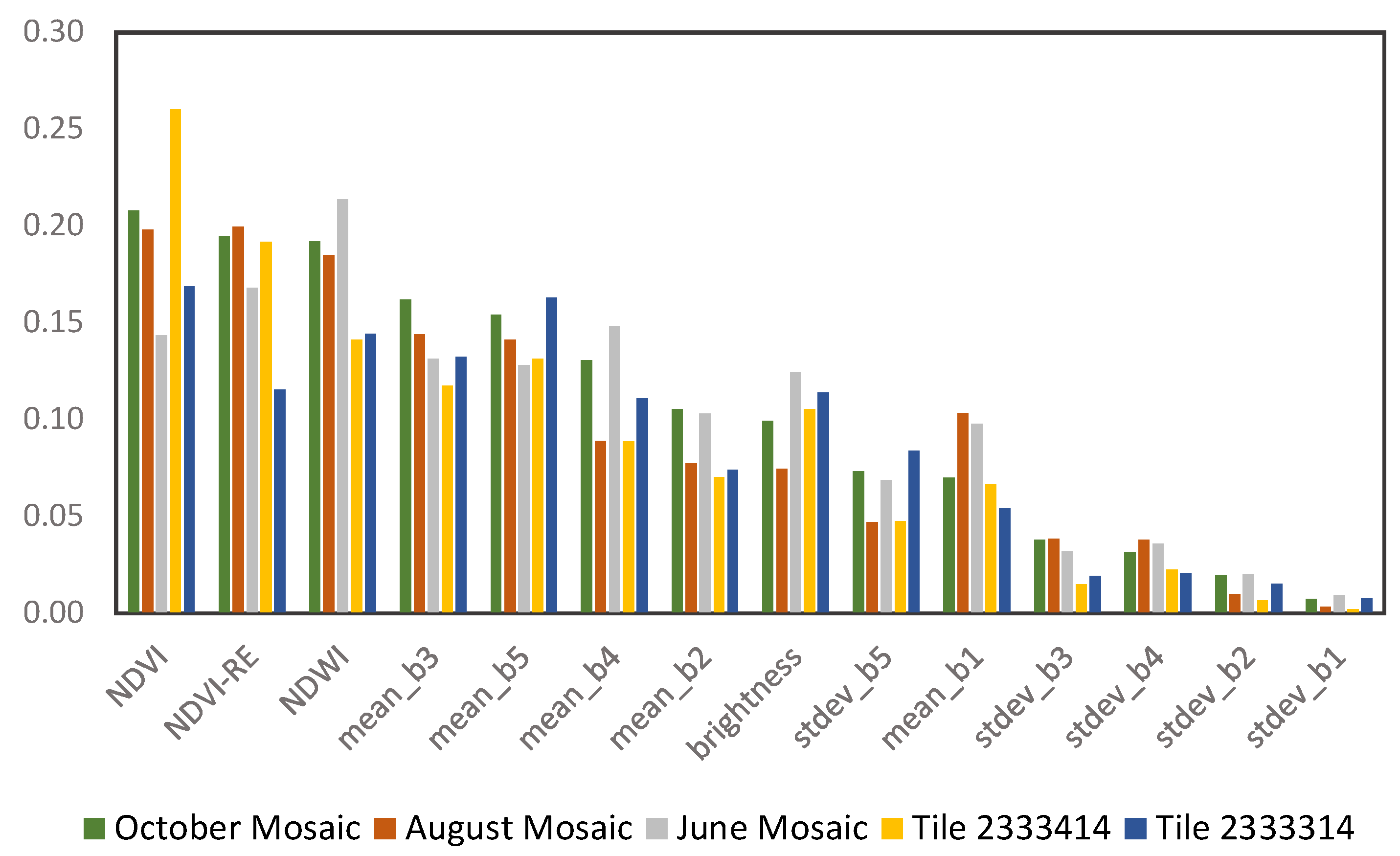
Table 2. Summary of selected features used in the random forest model. NDVI: Normalized Difference Vegetation Index; NDVI-RE: Normalized Difference Vegetation Index with red-edge band; NDWI: Normalized Difference Water Index.
Selected Features/StatisticsDescription
BrightnessSum of mean values of all layers (spectral bands) divided by the total number of spectral bands
Mean ValueMean (reflectance) value of each spectral band within an image object
Standard Deviation ValueStandard deviation (reflectance) value of each spectral band within an image object
Customized Attributes
NDVI(NIR–Red)/(NIR+Red)
NDVI-RE(RedEdge–Red)/(RedEdge+Red)
NDWI(Green–NIR)/(Green+NIR)
Table 3. Spatial contextual rules used to characterize LCCS land cover classes into physiognomic types; rules and classes with “*” were only applied for the Taquara watershed site, and rules with “**” were only applied for the Western Bahia site due to the absence of these classes in the other study site.
Level 1 ClassesSpatial RulesLevel 2 Classes
Closed Canopy1. Within hydromorphic soilsRiparian Forest
2. Within steep slopes (>20%) and not adjacent to perennial streams and water (relative border to ‘streams’ = 0) **Seasonally Dry Tropical Forest **
3. Adjacent to streams and water (relative border to ‘streams’ > 0)Riparian Vegetation
4. Within high elevation (>670 m) and flat terrain (slope < 8%) **Semi-Deciduous Forest **
Open Canopy1. Within hydromorphic soilsPalm Swamp
2. Within steep slopes (>20%) **Seasonally Dry Tropical Forest **
3. All other conditionsCerrado Woodland
Dense Shrub1. Within hydromorphic soilsShrub Swamp
2. All other conditionsSavanna
Open Shrub1. Within hydromorphic soilsShrub Swamp
2. All other conditionsOpen Savanna
Scrub–Shrub1. Within hydromorphic soils **Shrub Swamp **
2. All other conditions **Scrub Cerrado **
Herbaceous (wet)1. Within hydromorphic soilsMarsh
2. Within steep slopes (>20%) **Shade **
3. All other conditionsNon-Natural/Barren
Herbaceous (dry) Grassland *
Herbaceous Invasive Forbs and Shrubs *
Water1. Isolated small objects (size < 60 pixels) not within hydromorphic soils **Shade **
2. Within steep slopes (>20%)Shade **
2. All other conditions **Water **
Shrub–Herbaceous Semi-Natural Shrubby Grassland **
Soil, NPV ***, impervious surfaces (bright) Non-Natural/Barren
Soil, NPV ***, impervious surfaces (dark)
*** Non-photosynthetic vegetation.
Table 4. Error matrix (reported in ha), overall accuracy, producer’s accuracy, and user’s accuracy for the Western Bahia Level 1 LCCS classification. The number in parentheses corresponds to the number of independent test samples used for validation.
Closed Canopy (125)Dense Shrub (90)Herbaceous (Wet) (50)Open Canopy (125)Open Shrub (100)Scrub–Shrub (59)Shrub–Herb (50)Soil, NPV, Impervious (Bright) (30)Soil, NPV, Impervious (Dark) (46)Water (50)
Closed Canopy17.80.102.000.50000
Dense Shrub015.80.10.52.30.20.4000
Herbaceous (wet)0012.60.20.500000
Open Canopy0.71.70.513.900.30000
Open Shrub01.51.8013.90.30.6000
Scrub–Shrub0.70000.47.60.2000
Shrub–Herb00000.706.80.100
Soil, NPV, Impervious (bright)0000000.32.81.90
Soil, NPV, Impervious (dark)0000000.90.19.60
Water0010000007.7
Overall Accuracy (%)84.4
Producer’s Accuracy (%)92.5%82.4%81.3%83.6%77.7%86.1%74.4%95.4%83.6%100%
User’s Accuracy (%)87.3%81.7%94.5%80.8%77.1%85.2%89.7%56.6%91.0%93.3%
Table 5. Error matrix (reported in ha), overall accuracy, producer’s accuracy, and user’s accuracy for the Western Bahia Level 2 classification. The number in parentheses corresponds to the number of independent test samples used for validation.
Cerrado Woodland (50)Marsh (50)Non-Natural/Barren (76)Open Savanna (74)Palm Swamp (50)Riparian Forest (50)Savanna (75)Scrub Cerrado (50)Semi-Deciduous Forest (50)Shrubby Grassland
(50)
Shrub Swamp (50)Tropical Dry Forest (50)Water (50)
Cerrado Woodland6.200000.20.70.30.10000
Marsh012.6000.2000000.500
Non-Natural/Barren0014.30000001.2000
Open Savanna00011.7001.30.300.6000
Palm Swamp0.10.5005.00.400000.700
Riparian Forest0.200005.900000.300
Savanna0001.50015.200.30.4000
Scrub Cerrado0000.4000.06.70.60.2000
Semi-Deciduous Forest0.4000000.10.28.50000
Shrubby Grassland000.10.7000006.8000
Shrub Swamp01.9000.20.10.10005.000
Tropical Dry Forest0.3000000.400007.10
Water00.600000000007.7
Overall Accuracy (%)87.6
Producer’s Accuracy (%)85.8%81.3%99.5%81.8%92.4%89.4%85.5%89.5%89.4%74.4%77.3%100%100%
User’s Accuracy (%)81.7%94.5%92.5%84.4%75%92.3%87.5%84.2%92.9%89.7%69.2%91.4%93.3%
Table 6. Estimate of landscape composition for the Western Bahia site considering the proportion of the mapped area of each physiognomic type, reported in percentage, with respect to the total mapped area (i.e., entire study site extent) and for each individual image/mosaic.
Total (%)September 13th ImageSeptember 16th ImageJune MosaicAugust MosaicOctober Mosaic
Cerrado Woodland4.94.23.27.01.75.9
Marsh1.20.20.00.31.42.9
Non-Natural/Barren26.614.531.611.533.243.9
Open Savanna26.235.932.122.937.215.5
Palm Swamp0.80.10.10.20.72.0
Riparian Forest1.10.40.41.30.81.4
Savanna26.239.414.640.011.120.9
Scrub Cerrado1.90.00.04.41.20.0
Semi-Deciduous Forest1.50.50.13.40.40.2
Shade0.10.00.00.30.10.0
Semi-Natural Shrubby Grassland8.04.217.16.310.46.6
Shrub Swamp0.60.10.10.51.30.2
Seasonally Dry Tropical Forest0.60.20.41.50.10.0
Water0.30.50.30.20.30.3

