Abstract
When forest conditions are mapped from empirical models, uncertainty in remotely sensed predictor variables can cause the systematic overestimation of low values, underestimation of high values, and suppression of variability. This regression dilution or attenuation bias is a well-recognized problem in remote sensing applications, with few practical solutions. Attenuation is of particular concern for applications that are responsive to prediction patterns at the high end of observed data ranges, where systematic error is typically greatest. We addressed attenuation bias in models of tree species relative abundance (percent of total aboveground live biomass) based on multitemporal Landsat and topoclimatic predictor data. We developed a multi-objective support vector regression (MOSVR) algorithm that simultaneously minimizes total prediction error and systematic error caused by attenuation bias. Applied to 13 tree species in the Acadian Forest Region of the northeastern U.S., MOSVR performed well compared to other prediction methods including single-objective SVR (SOSVR) minimizing total error, Random Forest (RF), gradient nearest neighbor (GNN), and Random Forest nearest neighbor (RFNN) algorithms. SOSVR and RF yielded the lowest total prediction error but produced the greatest systematic error, consistent with strong attenuation bias. Underestimation at high relative abundance caused strong deviations between predicted patterns of species dominance/codominance and those observed at field plots. In contrast, GNN and RFNN produced dominance/codominance patterns that deviated little from observed patterns, but predicted species relative abundance with lower accuracy and substantial systematic error. MOSVR produced the least systematic error for all species with total error often comparable to SOSVR or RF. Predicted patterns of dominance/codominance matched observations well, though not quite as well as GNN or RFNN. Overall, MOSVR provides an effective machine learning approach to the reduction of systematic prediction error and should be fully generalizable to other remote sensing applications and prediction problems.
1. Introduction
As forest ecosystems are pushed toward novel conditions by anthropogenic disturbance and environmental change, there is an increasing need for information on the spatial distribution and condition of forest resources as a basis for quantifying ecosystem services, evaluating and forecasting change, and planning management actions. Field data and specifically forest inventory measurements can provide great detail at high accuracy, but are collected from a sample of small plots. Observational data are needed across scales relevant to forest policy and management, and commensurate with drivers of change acting over local to global scales (e.g., non-native pests, market conditions, climate change). Consequently, forest conditions are mapped from empirical relationships between field measurements and remote sensing data, often using some form of regression algorithm (e.g., [1,2,3,4,5,6]). Spatial heterogeneity of forests and uncertainty in remotely sensed predictor variables, however, can cause patterns of prediction error that may be detrimental to map use [6,7,8].
At moderate spatial resolutions, a prominent source of uncertainty in predictor variables may be physical differences in measurements between field plots and image pixels [7]. Whereas the ideal remotely sensed predictor data would represent the same ground area as reference plot data, scale and location mismatches introduce uncertainty. Forest inventory measurements are typically obtained over plots that are a fraction of the size of moderate resolution image pixels. For example, the Forest Inventory and Analysis (FIA) Program of the U.S. Forest Service provides measurements from a national network of field plots, each composed of a cluster of four subplots [9]. An FIA plot samples an area roughly equivalent to a 3 × 3 neighborhood of 30 m Landsat pixels. The actual area measured within subplots however, collectively equates to only 8% of that pixel neighborhood. Average conditions across a pixel neighborhood likely will not correspond to those measured at FIA subplots [7,8]. Image georeferencing or registration error coupled with GPS error in plot coordinates further interferes with the physical correspondence of pixels and plots [7]. Potentially compounding these problems are differences in timing between image acquisitions and plot measurements and additional sources of predictor uncertainty associated with remote sensing platforms, instrumentation, viewing conditions, and data handling.
Without correcting for uncertainty in predictor variables, regression algorithms generally assign variation in the predictors to variation in the response given the predictors. Minimization of prediction error when fitting regression models thereafter leads to underestimation of the strength of the relationship between predictors and response, and a characteristic pattern of prediction error where low values tend to be overestimated, high values underestimated, and variability suppressed. This pattern of error is known as regression dilution or attenuation bias [10,11]. In the presence of predictor variable uncertainty, reduction of total error tends to cause elevated attenuation bias. Attenuation is perhaps most detrimental to applications that are specifically dependent upon or influenced by patterns of prediction at high or low values, although more generally, the effects of attenuation bias may be difficult to identify or correct.
Attenuation bias is a long-recognized problem in remote sensing [12], but there remain few options available for its reduction or correction. Rejou-Mechain et al. [8] emphasized the importance of attenuation bias in the estimation of aboveground biomass by regression against field plot measurements, and demonstrated that established statistical approaches to reducing bias may be inadequate. Xu et al. [7] asserted that attenuation bias is a pervasive problem in remote sensing of forest attributes and suggested that no analytical method was capable of eliminating this bias. After analyzing causes using simple error models, they suggested that field data be collected over an area similar to the size of pixels or pixel neighborhoods used for prediction. Yet they also demonstrated that location mismatches can cause severe attenuation regardless. Robinson et al. [13] recognized strong attenuation bias when estimating aboveground biomass from FIA plot data and airborne radar, and suggested that FIA plots may not provide suitable reference observations. However, FIA or similar inventory data provide statistically representative and quality assured measurements that are commonly used for model training, though often resulting in patterns of error consistent with attenuation bias (e.g., [1,2,14,15,16,17]). A number of approaches have been advanced to reduce attenuation bias in parametric species distribution models, using error-in-variables [18] or Bayesian methods [19,20]. These approaches, however, are not always tractable for remote sensing applications, which frequently utilize very large sets of predictor variables.
Here we present an approach to the reduction of attenuation bias using support vector machines (SVMs). SVMs were originally developed for binary classification but have been widely applied to regression problems and remote sensing applications [21,22]. SVMs require the specification of several free parameters that determine model fit. Optimal values are problem-specific, varying with the available training data and predictor variables. SVM parameterization is therefore equivalent to a search for an optimal combination of values within a multidimensional search space. The complexity of the problem is further increased if the search is expanded to include the selection of a subset of predictor variables. Variable selection may reduce computational complexity and improve model fit [23], and because different predictor variables may be subject to different levels of measurement error, variable selection may also reduce systematic error. Similar benefits may follow from the selection of a subset of available training data [24]. Ideally, all aspects of model specification are performed simultaneously, and several classes of optimization or search algorithms are suitable, including genetic algorithms (GAs; e.g., [25,26,27,28]). Using a guided search mechanism founded on the analogy of evolution by natural selection, GAs are capable of obtaining near-optimal solutions from a large and complex search space [29]. Because attenuation arises from the minimization of error when fitting regression models in the presence of predictor variable uncertainty, we approached SVM model training and model selection as a multi-objective optimization problem, simultaneously minimizing total and systematic error using a multi-objective GA [30]. Our goal was to obtain solutions with reduced systematic error at acceptable levels of total error.
Our interest in attenuation bias stemmed from the need to map individual tree species distributions to improve knowledge of current forest conditions and to forecast future conditions in the Acadian Forest of northern Maine (USA). Reliable predictions of tree species distributions are needed, and patterns of species dominance or codominance are particularly important. We applied our multi-objective support vector regression (MOSVR) method to the prediction of forest tree species relative abundance (proportion of aboveground live biomass) in the Acadian Forest using multitemporal Landsat imagery and topoclimatic variables. We evaluated species dominance and codominance in terms of ranked relative abundance, and compared relative abundance and dominance/codominance predictions against those of other commonly used modeling approaches including random forests and nearest neighbor methods. Results indicated that MOSVR provides an effective approach to the reduction of attenuation bias.
2. Materials and Methods
2.1. Study Area
The Acadian Forest Region of the northeastern U.S. occupies a transition zone between the northern boreal forest and the southern temperate deciduous-dominant forest [31], and includes approximately 4 Mha of nearly contiguous, undeveloped forestland across northern and western Maine. Our 1.9 Mha study region (Figure 1) was defined by the overlap of Landsat Worldwide Reference System path 12, row 28 and the political boundary between northwestern Maine and Quebec, Canada. Topography is generally flat or rolling with occasional low mountains and an extensive network of rivers, lakes, and wetlands. Tree species diversity is relatively high as the northern limit of southern species overlaps with the southern limit of northern species [32].
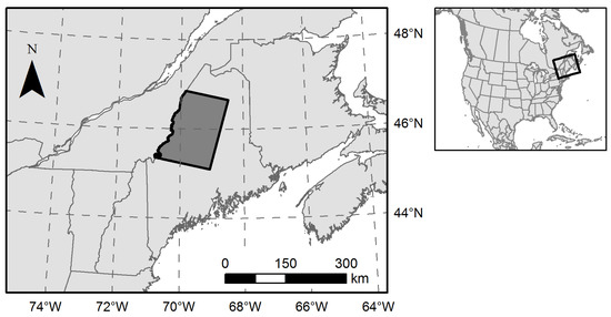
Figure 1.
Northern Maine, USA study area encompassing 1.9 Mha of forestland. Political boundaries were obtained from the North American Atlas (Natural Resources Canada, Instituto Nacional de Estadística Geografía e Informática, and U.S. Geological Survey).
Forest type distributions are associated with climatic gradients, topo-edaphic conditions, and disturbance history [33]. Northern hardwood species (Acer saccharum, Betula alleghaniensis, Fagus grandifolia) predominate across lower hilltops and at mid-slope. Spruce-fir species (Abies balsamea, Picea rubens, P. mariana) predominate where soil or microclimatic conditions exclude the more demanding hardwoods. Mixedwood stands commonly occur along ecotones or as a result of succession following disturbance. Shade-intolerant hardwood species (Betula papyrifera, Populus spp.) are commonly found following intense disturbance.
2.2. Reference and Predictor Data
Predictive models of species relative abundance are based on reference data provided by the USFS FIA Program. The contemporary network of field plots adheres to an equal probability sampling design, with plots randomly located within 2428 ha hexagonal tiles [9]. The FIA program maintains the confidentiality of true plot locations to protect the privacy of landowners and to preserve plot integrity [34]. True locations were made available for use through a collaborative agreement with the USFS Northern Research Station FIA Program. Tree measurement data were used to calculate species relative abundance as a proportion of estimated live aboveground biomass (stems >2.54 cm diameter, measured at 1.37 m; DRYBIO_AG variable [35]). Since 1999, 20% of plots within Maine have been surveyed annually during 5-year inventory cycles [9].
Our intention was to map forest conditions of the early or mid-2000s to support analysis of recent change as well as forecasting of future conditions. We collected Landsat Thematic Mapper (TM) and Enhanced Thematic Mapper Plus (ETM+) imagery acquired at different times throughout the growing season (late April through early October) to exploit species-specific phenological patterns as a basis for improving species predictions. Frequent and extensive cloud cover dictated the use of both TM and ETM+ images, and we elected to use ETM+ images acquired during the early 2000s prior to the failure of the ETM+ scan line corrector. We selected eight relatively cloud- and snow-free images acquired from 2001-2006, roughly matching a 5-year FIA inventory cycle (Table 1). Images were obtained from the U.S. Geological Survey (USGS) Earth Resources Observation and Science Center and the Multi-Resolution Land Characteristics Consortium at 30 m resolution with standard terrain correction applied. Bands 1-5 and 7 (visible and reflective infrared) were extracted for further processing and converted to top-of-atmosphere reflectance to facilitate cloud masking and interpretation of pixel values during image preparation (conversion was not required for predictive modeling). Clouds and cloud shadows were masked using a semi-automated procedure developed in-house, verified and corrected by visual interpretation and on-screen digitization. Visible snow cover in early-season imagery was masked by unsupervised classification using an ISODATA algorithm and visual interpretation of snow-covered classes. Images were then corrected for topographic illumination effects using the SCS+C algorithm [36], with slope and aspect calculated from the 1 arc-second (30 m) National Map Seamless Digital Elevation Model maintained by the USGS [37].

Table 1.
Landsat images used for predictive modeling of tree species relative abundance. Images were acquired over Landsat Worldwide Reference System-2 path 12, row 28, and were obtained from the U.S. Geological Survey Earth Resources Observation and Science Center unless indicated otherwise.
Forest canopy change during the 5-year observation period dissociated image characteristics from field measurements at affected plot locations. We therefore masked locations of apparent canopy cover change using available leaf-on images acquired in 2001, 2004, and 2007 (Table 1). The iteratively-reweighted multivariate alteration detection transformation [38] was applied to 2001–2004 and 2004–2007 image pairs to estimate a probability of spectral change during each interval. Intervals were combined by selecting the maximum probability of change, and a threshold was selected so that 20% of forest pixels were identified as change pixels. Threshold selection was based on visual inspection of the resulting 2001-2007 change mask against Landsat imagery, which indicated close correspondence with canopy disturbance and visible regrowth in previously disturbed stands.
Additional spatial predictor variables included climate and terrain attributes thought to be relevant to tree establishment or growth. Terrain data included 10 morphometry, 8 lighting/visibility, and 11 hydrology variables (Table 2) calculated from the 1 arc-second (30 m) National Map Seamless Digital Elevation Model and the National Hydrography Dataset (NHD) using the System for Automated Geoscientific Analyses [39]. Elevation data was smoothed with a Gaussian filter to reduce the effects of random error and systematic artifacts (circular filter element, radius = 90 m, σ = 1.5). Terrain slope, aspect, and curvature were calculated from a second-order polynomial fit [40]. Direct insolation was calculated at mid-month, April-September, by assuming a uniform 65% atmospheric transmittance, a value that produced insolation estimates in good agreement with a previously published regional climate model [41]. Hydrology variables including catchment area, flow path length, and distance to stream channel were calculated using a bidimensional flow routing algorithm [42] after filling sinks in the elevation data [43]. Synthetic stream channel networks were derived from the catchment area raster after masking and dilating NHD water bodies using a 5 × 5 filter element. The dilated water body mask reduced the tendency for channels to initiate near the edges of water bodies, where the flow routing algorithm produced large estimates of flow accumulation. Climate data were obtained from the USDA Forest Service Rocky Mountain Research Station, Moscow Forestry Sciences Laboratory, and included 17 variables (Table 2) derived from monthly temperature and precipitation surfaces interpolated from weather station data for the climate normal period of 1961–1990 [44,45]. Climate data were available at approximately 1 km spatial resolution.
Table 2.
Terrain and climate variables used to model and map tree species relative abundance. Terrain variables were calculated using the System for Automated Geoscientific Analyses software [39] v. 2.1.4 with default settings unless otherwise specified. Climate variables were obtained from the USDA Forest Service Rocky Mountain Research Station, Moscow Forestry Sciences Laboratory [44].
Predictor variable values were extracted at forested FIA plots. Landsat and terrain data were compiled by averaging values from forest pixels within 3 × 3 neighborhoods surrounding plot centers; climate predictor data were extracted as 1 km pixel values. Forest pixels were differentiated from non-forest using the 1993 Maine Gap Analysis Program (GAP) land cover map, augmented with the agricultural classes of the 2001 National Land Cover Database (NLCD). The 1993 GAP map differentiated forest from non-forest with an estimated 100% accuracy in our study area [49]. Incorporation of the 2001 NLCD agricultural classes accounted for a small amount of land cover change predating our 2001-2006 observation period. SVMs are generally incapable of working with incomplete predictor data and for the purposes of algorithm development and evaluation, we elected to exclude samples with missing data due to forest cover change, cloud/shadow cover, or snow cover rather than incorporate an additional algorithm for imputing missing data. Remaining plot locations yielded a training/validation data set consisting of 349 samples.
2.3. Multi-Objective SVR (MOSVR) Algorithm Description
Our implementation of a multi-objective SVR (MOSVR) algorithm is based on ε-SVR with a Gaussian radial basis function (RBF) kernel, and includes parameter selection (γ, ε, and C), variable selection, and a form of training sample selection. The kernel function accommodates nonlinear relationships through the projection of training data into a space of high dimensionality. The RBF kernel typically performs well due to several computational and practical advantages over other functions, including the need to specify only a single free parameter, the kernel width γ [22,50]. Narrower RBF kernels essentially permit the projection of training data into higher dimensions, corresponding to more complex solutions when expressed in the original variable space. The ε-SVR formulation is based on the so-called ε-insensitive loss function, where a margin of width ε bounds the regression function, with nonzero loss applied only to training samples lying outside the margin (the support vectors, or SVs). Narrower margins generally correspond to larger numbers of SVs and more complex solutions. The regularization or penalty error parameter C specifies a trade-off between model complexity and training error. The parameters ϵ, C, and γ collectively determine the complexity of the regression function and its ability to generalize to new data [50]. Optimal values are problem-specific, varying with the available training data and predictor variables. MOSVR executes a simultaneous search for parameter values, predictor variable subsets, and training sample subsets. Our approach to training sample selection is to specify a subset of reference samples as eligible for exclusion from model training. However, all reference samples are used for model validation.
Use of a GA requires the expression of individual models in the form of a genotype subject to selection, genetic recombination, and mutation. Each SVR model is represented by a bit string chromosome, composed of segments encoding parameter values, variable selection, and sample exclusion (Figure 2). The lengths of segments representing parameter values determine the levels of precision with which real values are represented by binary encoding. Variable selection is encoded as a bit string segment with length equal to the number of available predictor variables, interpreted as a binary mask. Sample exclusion is similarly encoded as a segment with length equal to the number of samples made eligible for exclusion, indicating specific samples to be excluded from model training. Note however, that all samples are used for model validation within a cross-validation (CV) procedure. The GA is initiated with a uniform random population of a user-specified size.
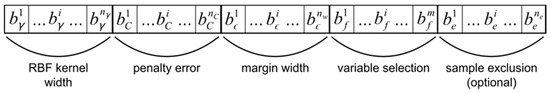
Figure 2.
Genetic algorithm chromosome design. Bit string chromosomes are composed of segments encoding model parameter values, predictor variable selection, and training sample exclusion.
Numerous multi-objective GAs have been published and reviewed [30]. Our approach is based on the popular NSGA-II algorithm [51] implemented in the MATLAB Global Optimization Toolbox, Release 2014a (The MathWorks, Inc., Natick, MA, USA). The LIBSVM open source software [52] is used for SVM training and prediction. The MATLAB implementation of NSGA-II acts as a wrapper for LIBSVM. A diagrammatic representation of algorithm details is provided in Figure 3.
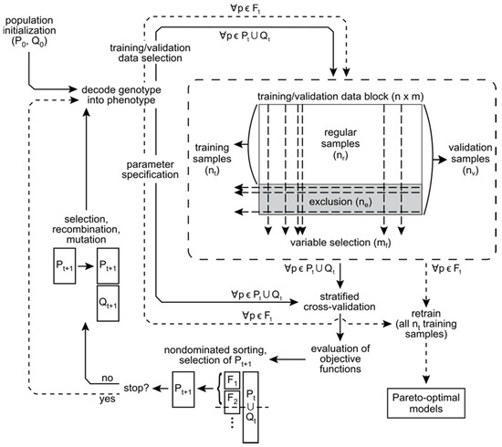
Figure 3.
Multi-objective support vector regression algorithm implementation. Following selection of training and validation data, SVR models are fit and predictions made using LIBSVM. Objective function values are estimated by repeated cross-validation using all samples, and serve as the basis for population sorting, parent selection, and genetic operations embedded within the NSGA-II.
For each generation of solutions, NSGA-II differentiates groups of parents (P) and offspring (Q) of equal size. Initially all individuals are random and specification of P0 and Q0 is arbitrary. The chromosome representing each member of the current population (Pt ∪ Qt) is decoded into real-valued SVM parameters and variable selection and sample exclusion masks. Individual models are trained and validated by a k-fold CV. Continuous variables are scaled to unit range ([0, 1]) at each CV iteration. The CV procedure is repeated a user-specified number of times and results averaged to reduce the uncertainty of objective function estimates [53].
CV estimates of objective function values are assigned to each member of the current population. Objective functions quantify total error (RMSET) and systematic error (RMSESYS):
where a and b are the intercept and slope of the ordinary least squares (OLS) regression between predicted values and observed values yi [54]. The objective functions map solutions into a two-dimensional objective space Φ = {g1(p) g2(p) | p ϵ Ω}, where Ω is the set of all possible solutions. Solution pi is said to dominate solution pj provided g1(pi) ≤ g1(pj) and g2(pi) ≤ g2(pj) with at least one strict inequality. In other words, one solution dominates another if it is better in one objective and at least as good in the other. A solution is nondominated if neither objective can be improved further without a worsening of the other. The set of nondominated solutions in Ω is referred to as the Pareto set, and the image of the Pareto set in the objective space Φ is the Pareto front. The goal of NSGA-II is to closely approximate the true Pareto set by driving evolution toward the Pareto front.
At each generation, NSGA-II sorts the current population of solutions (Pt ∪ Qt) into a sequence of nondominated fronts (F1, F2,…). The first front F1 includes all nondominated solutions from the total population and is the current best approximation of the Pareto front. Once F1 is obtained, these solutions are removed from the population, and the next front F2 is obtained as nondominated solutions from the reduced population. The process is iterated until all population members have been assigned to a front. NSGA-II subsequently identifies one half of the population as the next generation of parents (Pt+1), selecting solutions from successive fronts. In the MATLAB implementation, the maximum number of parent solutions selected from F1 and successive fronts is constrained in order to promote population diversity throughout algorithm execution. Within any individual front, parent solutions are selected from sparse or less crowded portions of the front to further promote population diversity.
The next generation of offspring (Qt+1, equal in size to Pt+1) are obtained through genetic recombination and mutation of parent solutions. A user-specified proportion of offspring are produced through genetic recombination of a pair of parent solutions, and the remainder through mutation of a single parent. Individual parents are identified by tournament selection [55], where a user-specified number of solutions are randomly selected from Pt+1 and the best is selected as a parent. Better solutions lie on lower ranked fronts and in less crowded regions along their front. Genetic recombination occurs through a crossover operation in which an offspring is constructed from bit string segments copied from its parents. Different crossover operations determine the manner in which information is exchanged and the potential degree of novelty introduced through exchange [55]. An offspring produced by mutation is a copy of its parent subjected to a mutation operation that switches individual bit values with a user-specified probability. Once offspring have been produced, parent and offspring chromosomes (Pt+1 ∪ Qt+1) are decoded and the process repeats over a user-specified number of generations. At the final generation, members of F1 are retrained using all available training samples and returned as a set of Pareto optimal models expressing tradeoffs between RMSET and RMSESYS.
2.4. MOSVR Algorithm Execution
From the FIA data compiled for our study area, we modeled and mapped the relative abundance of 13 tree species (Table 3). SVR parameter values were constrained within reasonable ranges (log(γ) ϵ [–4,0]; log(C) ϵ [–1,3]; log(ϵ) ϵ [–4,0]). A set of 78 reference samples was made eligible for exclusion from model training, including plots with non-forest cover types identified by FIA records and plots with high spectral variability (based on neighborhood standard deviations, averaged across all images and bands). We retained samples for which FIA records indicated multiple forest types. All reference samples were used for model validation in a 10-fold, 10 times repeated CV.
Table 3.
Reference data characteristics of the 13 modeled tree species (349 samples).
We set GA parameters in an effort to balance the promotion of population diversity against execution time. The population size was set to 500, with a maximum of 20% of solutions maintained on the approximate Pareto front. Parents were selected by tournament with 10 participants. 70% of offspring were generated by crossover of parent chromosomes, using the MATLAB scattered crossover operation in which bits were selected from each parent at random. 30% of offspring were generated by mutation of parents, with a mutation rate of 2.5%. Approximate Pareto fronts typically stabilized by 80-100 generations, and algorithm execution was limited to 120 generations.
The estimation of RMSESYS by linear least squares regression of CV predictions onto observed values was in some cases sensitive to outlying samples whose CV predictions deviated strongly from those of other samples with similar observed values. In these cases, removal of influential outliers was required to ensure that a small number of samples did not drive the GA toward less desirable solutions, where reduced RMSESYS reflected the presence of influential outliers rather than trends across the larger set of reference data. We implemented an automated outlier removal strategy at 30, 60, and 90 generations based on the identification of influential outliers for each member of the F1 front. Outlying samples were identified by applying a threshold to absolute studentized residuals. Influential outliers were identified as those whose removal resulted in a change in RMSESYS exceeding a threshold level, when expressed as a proportion of RMSET. Samples identified as influential outliers in the majority of F1 solutions were removed from both training and validation data. For most species, we applied a residual threshold of 3 and a RMSESYS threshold of 1%. For FRAXI, PIMA, and TSCA we used more conservative threshold values of 4 and 2% to reduce the number of outliers removed. The number of outliers removed for each species ranged from zero to seven, and averaged four (Supplementary Table S2).
At the end of MOSVR execution, an individual solution was selected from the midsection of the Pareto front where solutions represented a compromise between RMSESYS and RMSET. We selected the model positioned nearest to the origin after unit-scaling RMSESYS and RMSET values to normalize for differences in magnitude between the two.
2.5. Model Comparisons
We compared MOSVR results to those obtained from random forest (RF) [56], gradient nearest neighbor (GNN) [16], and random forest nearest neighbor (RFNN) [57] algorithms. RF is an ensemble algorithm based on regression trees and has been widely applied in species distribution modeling and remote sensing applications. GNN was originally developed and has been commonly applied as a k = 1 nearest neighbor algorithm for modeling regional tree species distributions, with proximity calculated within a feature space defined by a canonical correspondence analysis (CCA) of plot measurements and image or environmental predictor data. With k = 1, all observations from individual reference plots are imputed to pixels, retaining plot-level species associations in predictions. RFNN is another k = 1 nearest neighbor variant, with proximity obtained from the nodes of one or more RF models. RFNN shares the advantages of GNN, but is based on a novel, non-Euclidean proximity metric that may lead to improved outcomes [58].
We adopted typical parameter settings and execution strategies using R v 3.0.3 [59]. RF models were fit with the R package randomForest, v 4.6-12 [60], with an ensemble size of 2000 and default parameter settings (mtry = one third of the number of predictor variables; nodesize = 5). For GNN, CCA models were first fit with the R package vegan, v 2.4-3 [61] using the relative abundance of all species as the multivariate response. Following Ohmann and Gregory [16], we performed a forward stepwise variable selection procedure based on AIC, permutation testing, and a check of variance inflation factors. Variables were considered for addition in the order of their contribution to constrained inertia (equivalent to AIC when all variables are continuous). Variables were added provided they were deemed significant by a permutation test (p = 0.01, 99 permutations) and all variance inflation factors remained below 20. Nearest neighbor imputation was based on Euclidean distance calculated from the first seven CCA axes (accounting for >95% of total variation explained), scaled by their constrained eigenvalues. GNN imputation, and execution of the RFNN algorithm, was performed using the R package yaImpute, v 1.0-26 [57]. The RFNN imputation was based on a combined nodes matrix obtained by three separate RF models, fit to total live aboveground biomass, the species with maximum relative abundance based on aboveground live biomass, and the relative abundance of that species.
We also implemented a single-objective approach to SVR model training (SOSVR) using a traditional GA (MATLAB Global Optimization Toolbox, Release 2014a) minimizing RMSET, because SVR model selection is typically based on minimization of overall prediction error. Finally, to evaluate the relative benefits of variable and sample selection strategies employed by MOSVR, we compared results to two alternative MOSVR execution strategies that included parameter selection only, and parameter plus variable selection but no sample selection. All MOSVR execution strategies used the same GA settings and the same outlier removal strategy. SOSVR runs were executed using the same values for applicable GA settings, and included parameter, variable, and sample selection.
Following model selection/parameterization, models of all types were run through a 10-fold CV 100 times with different random partitions to obtain mean model performance metrics from CV predictions. To ensure fair comparisons amongst model types, we removed CV predictions associated with influential outliers in MOSVR, on a species by species basis, ensuring equal validation samples. We compared mean model performance metrics (RMSET, RMSESYS, OLS linear slope, and R2) and 95% confidence intervals under the assumption that metrics obtained by repeated CV were approximately normal. We considered a species dominant if it occurred as one of the three most abundant species, and we calculated the frequencies with which any species or pair of species occurred as dominant or codominant. Mean dominance/codominance frequencies and corresponding 95% confidence intervals were obtained from CV predictions for each model type and compared to observed values.
3. Results
The approximate Pareto fronts obtained by MOSVR generally shared a common geometry. Solutions were distributed more or less evenly across a curvilinear front, with incremental change in one objective balanced by incremental change in the other (Figure 4a). At one end, models had low total error but comparatively high systematic error (e.g., Model 1), apparent as a deviation from the 1:1 relationship between predicted and observed values (Figure 4b). At the other end, models had low systematic error but comparatively high total error (e.g., Model 3, Figure 4d). Fronts were convex toward the origin (Figure 4a) such that nearer to either end the value of one objective function changed much more quickly than the other. Rather than select models with minimal systematic error from one end of the front, where small decreases in RMSESYS were associated with large increases in RMSET, we selected models from the midsection where prediction error represented more of a compromise between systematic and total error (e.g., Model 2, Figure 4c).
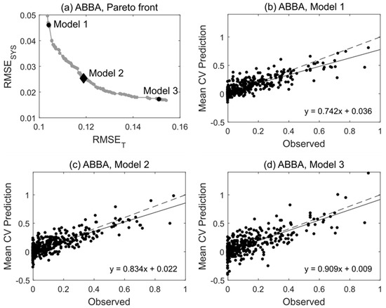
Figure 4.
Pareto front and select Pareto-optimal models for species ABBA (balsam fir). (a) The approximate Pareto front obtained by MOSVR (including parameter, variable, and sample selection). (b–d) Plots of predicted vs. observed values for selected models lying at different positions along the Pareto front. For comparison to other prediction methods and for use in forest mapping, a model was selected from the midsection of the front (Model 2). Predicted values are mean values obtained from 100 repetitions of a 10-fold CV.
Of the three MOSVR execution strategies evaluated, the least systematic error was typically attained through the simultaneous selection of parameter values, variables, and samples (Supplementary Table S1). In a number of cases, parameter and variable selection achieved similar levels of systematic error, and in one case significantly lower systematic error. However, in all of these cases total error exceeded that achieved when sample selection was used as well. Parameter selection alone failed to reduce systematic error to similar levels. All MOSVR results presented hereafter were obtained with parameter, variable, and sample selection.
Several patterns appeared when comparing model performance metrics across model types and species (Figure 5). SOSVR attained the least total error for all but a single species (Figure 5a). The least systematic error, when expressed as a percentage of total error, was always attained by MOSVR (Figure 5b). The slope between predicted and observed values was also greatest (closest to one) for MOSVR models (Figure 5c). R2 values were generally greatest for MOSVR models as a result of reduced levels of systematic error, although the low total error attained by SOSVR resulted in R2 values as high or higher for some species (Figure 5d). In nearly all cases, nearest neighbor methods (GNN and RFNN) resulted in the greatest total error and RF models the greatest systematic error. Compared to MOSVR outcomes in which systematic error ranged from 10–42% of total error across species (mean = 27%), systematic error in RF models accounted for 62–93% of total error (mean = 83%). Systematic error in nearest neighbor methods ranged from 30–71% of total error (GNN mean = 58%; RFNN mean = 57%).
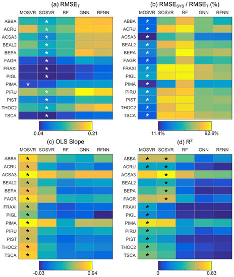
Figure 5.
Predictive performance by species and model type. Performance metrics were obtained from linear regression of CV predictions against observed values, averaged across 100 repetitions of a 10-fold CV. Asterisks indicate model types that produced either the best mean metric value for a given species or a value whose 95% confidence interval overlapped that of the best.
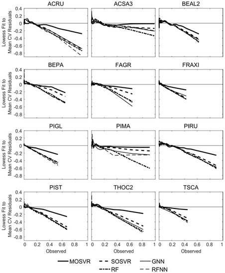
Patterns of systematic error summarized by model performance metrics and consistent with attenuation bias were apparent in residuals. Species ABBA provides a representative example (Figure 6). All model types typically produced slight overestimation of relative abundance for observed values <0.2, although in this case overestimation by MOSVR was negligible for relative abundance >0.05. All model types produced a systematic underestimation of relative abundance for observed values >0.2. The magnitude of underestimation increased as observed relative abundance increased. The level of apparent error at high abundance varied between models, with GNN producing the most and MOSVR the least (Figure 6f). The degree to which MOSVR mitigated attenuation bias varied from species to species (Figure 7). However, MOSVR always reduced the magnitude of systematic underestimation at the high levels of relative abundance that would presumably most influence predicted patterns of dominance/codominance.
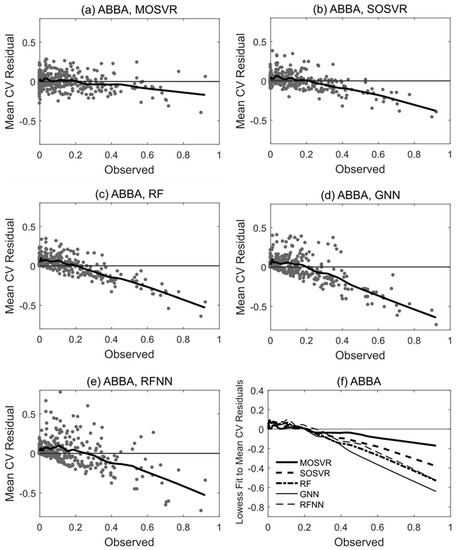
Figure 6.
Trends in residual values for selected model types fit to species ABBA (balsam fir). Residuals plotted against observed values for (a) MOSVR, (b) SOSVR, (c) RF, (d) GNN, and (e) RFNN model types. Residual values are mean values obtained from 100 repetitions of a 10-fold CV, displayed with lowess curves (local weighted least squares regression of a first degree polynomial, spanning 20% of samples). (f) Lowess curves fit to residual plots for direct comparisons between model types.
Patterns of observed dominance and codominance largely reflected species associations expected in the most prevalent forest types of the region (Figure 8a, Table 3). Elevated dominance/codominance of ABBA and PIRU were consistent with a high prevalence of upland spruce-fir. Similarly, dominance/codominance of ACSA3 and BEAL2, and to a lesser extent FAGR which occurs at lower abundance across our study area (Table 3), reflected a high prevalence of northern hardwood. BEPA commonly occurs at relatively high abundance following intense disturbance, which is common throughout much of our study area. ACRU grows in high abundance under a wide range of conditions, often in disturbed areas. A number of species are either not prevalent or not generally found at high relative abundance within our study area (FRAXI, PIGL, PIMA, TSCA) (Table 3).
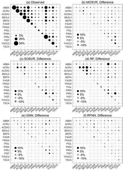
Figure 8.
Observed and predicted patterns of species dominance/codominance. (a) Observed dominance/codominance frequency, or the proportion of FIA plots at which a species or pair of species occurred or co-occurred as one of the three most abundant species. (b–f) Differences between predicted and observed dominance/codominance frequencies for (b) MOSVR, (c) SOSVR, (d) RF, (e) GNN, and (f) RFNN model types. Predicted values were calculated as mean values obtained from 100 repetitions of a 10-fold CV. The maximum width of corresponding 95% confidence intervals ranged from 0.4% for RF models to 0.7% for GNN.
Of the model types evaluated, nearest neighbor methods and RFNN in particular produced patterns of dominance and codominance that most closely conformed to those observed (Figure 8e,f). The maximum absolute difference between observed dominance/codominance frequencies and those predicted by GNN and RFNN was about 4% and 2%, respectively. Absolute differences averaged less than 1% for both. In contrast, both SOSVR and RF models resulted in predicted patterns that deviated from observations much more strongly (Figure 8c,d), with absolute differences averaging about 2% for each but exceeding 10% in a number of instances. The largest differences were over-estimates of codominance, and for RF several of these amounted to a near doubling of observed frequencies (e.g., ACRU and BEAL2, Figure 8d). MOSVR produced patterns much closer to those observed and to those predicted by the nearest neighbor methods, with a maximum absolute difference of about 6% and an average absolute difference of about 1%.
4. Discussion
Our goal was to develop a method of predicting individual tree species relative abundance from moderate resolution data at high accuracy and with low systematic error relative to other established approaches. Comparisons across 13 tree species indicated that our MOSVR algorithm accomplished that goal (Figure 5, Figure 6 and Figure 7). As expected, algorithms that yielded the lowest total prediction error (RF and SOSVR) also produced the greatest systematic error, consistent with a strong attenuation bias arising from predictor variable uncertainty. Although these methods effectively minimized mean prediction error, they did so at the cost of systematic over- and underestimation at low and high ends of observed data distributions. Underestimation at high relative abundance in particular appears to have affected predicted patterns of species dominance and codominance, causing strong deviations from those observed at FIA plots (Figure 8c,d).
In contrast, two k = 1 nearest neighbor methods (GNN and RFNN) reproduced observed dominance/codominance patterns with comparatively little error (Figure 8e,f). By simultaneously imputing reference measurements for all species, these methods retained plot-level relationships between species and reproduced dominance/codominance patterns most closely. However, total prediction error was comparatively high for individual species (Figure 5). Others have emphasized the strength of nearest neighbor methods in producing reliable community-level outcomes [16,62]. In this case, despite their reproduction of observed dominance/codominance frequencies, nearest neighbor methods yielded predictions of relative abundance with comparatively low accuracy, subject to strong attenuation bias.
MOSVR produced the least systematic error for all species, at levels of total error that were always less than nearest neighbor methods and often comparable to either SOSVR or RF (Figure 5). Predicted dominance/codominance frequencies agreed with observations much more closely than SOSVR and RF, though not quite as well as GNN or RFNN (Figure 8). Ultimately, by reducing systematic error in individual species models, MOSVR balanced the benefits of GNN and RFNN against those of SOSVR and RF.
MOSVR was able to achieve our primary objective of reducing systematic error by treating the minimization of both total and systematic error as model selection or tuning objectives within a multi-objective framework. Multi-objective model selection requires a statistical or machine learning model capable of generating diverse solutions through the controlled manipulation of model structure. SVMs are well-suited in the sense that manipulation of a few free parameters can dramatically alter the geometry of decision boundaries [50]. Pasolli et al. [28] previously implemented a multi-objective method for SVR parameter selection. For our species relative abundance problems, parameter selection alone failed to achieve desired reductions in systematic error (Supplementary Table S1). Meaningful reductions required additional complexity in model specification, achieved through the integration of variable and sample selection. Integration of variable selection into GA chromosome design enabled population diversification across a much larger search space, ultimately leading to the evolution of models with substantially reduced bias. Our sample selection mechanism led to further improvements in model performance in some cases, presumably for similar reasons. SVR models are directly determined by individual samples (SVs) lying on or outside margin boundaries. The removal or addition of an SV necessarily changes model fit, whereas removal of a sample lying within the SVR margin does not. We made certain samples eligible for exclusion based on an assumption that they were more likely to be SVs under a variety of model specifications due to observed variability in land cover or image characteristics. Enabling their exclusion further reduced bias or total error in some but not all cases (Supplementary Table S1).
Although MOSVR effectively reduced systematic error, there is room to question when this is necessary. Riemann et al. [17] presented a multi-scale comparison of biomass predictions made by a GNN variant against FIA plot measurements as a means of assessing model bias. A comparison of plot measurements and pixel-level predictions (250 m pixels) revealed strong systematic disagreement consistent with attenuation bias, but comparisons of averages across large spatial scales (78,100 and 216,500 ha) revealed low levels of systematic disagreement. Riemann et al. [17] interpreted this as evidence of an unbiased model, and specifically that systematic differences between plots and pixels were more attributable to validation data uncertainty than actual model error. However, attenuation bias does not degrade mean predictive accuracy and averages over large areas should be little affected. It seems plausible that large-area averages could agree well, despite substantial attenuation bias in the modeled plot-pixel relationships and substantial systematic error at the plot-pixel level. Riemann et al. [17] stated that strong systematic agreement of large-area averages provides evidence of an unbiased model under the unverified assumption that modeled relationships apply across scales. But modeled relationships could generally be expected to differ across scales of aggregation (i.e., the modifiable areal unit problem [63]). These considerations leave open the alternative interpretation that the GNN model was biased.
The question of whether systematic disagreement between plots and pixels should be considered evidence of model bias or a validation artifact has been explored in relation to predictor variable uncertainty. Xu et al. [7] examined the effects of predictor variable uncertainty in the context of ordinary linear regression. Using a field measurement protocol specifically designed to investigate the effects of mismatches in scale and location between plots and pixels, they compared prediction patterns against those expected from two types of predictor variable uncertainty. When the observed predictor W is a noisy realization of the true or ideal predictor X (W = X + U, where the error term U has zero mean and is independent of X such that E(W|X) = X), the Classical error model applies. This corresponds to the situation in which plots are larger than pixels, or a species responds to a long-term average but the corresponding predictor variable reflects a shorter time frame (as would be the case for our mid-month insolation predictors, for example). When the observed predictor is considered a smooth representation of the true or ideal predictor (X = W + U and E(X|W) = W), the Berkson error model applies. This corresponds to the situation in which plots are smaller than pixels, or a species responds to environmental conditions over a shorter timeframe than predictors represent (as may be the case when species are affected by extreme conditions that are not resolved by climatological predictors). Xu et al. [7] demonstrated that although Berkson error does cause apparent systematic error in cross-validation outcomes, that pattern is no longer present when predictions are compared to new reference observations made at the same scale. Linear models are not biased by Berkson error. In contrast, Classical error does cause strong attenuation bias of the model itself, affecting coefficients and introducing systematic error that does not go away when validation data are scaled to match pixels.
The Berkson model fits the situation in which moderate resolution predictors are paired with FIA plots, and the work of Xu et al. [7] would appear to validate the assertions of Riemann et al. [17] on those grounds. However, several factors virtually ensure that actual predictor error deviates from the Berkson model. Location mismatches caused by georeferencing or GPS error, for example, are best represented by a mixture of Classical and Berkson error and can cause attenuation bias more severe than Classical error associated with a scale mismatch [7]. Additionally, many applications build models using predictors with different patterns of uncertainty, some of which may be best represented by Berkson error and some by Classical error. For species distribution models that utilize environmental variables, the nature of predictor uncertainty may differ by species due to different responses to environmental conditions (e.g., differing sensitivity to extreme vs. average conditions). Finally, the analysis provided by Xu et al. [7] was based on ordinary linear regression. Both Berkson and Classical error can cause attenuation bias and systematic prediction error when models are nonlinear or nonparametric [64]. Not all systematic error in plot-pixel comparisons is indicative of model bias, but without a thorough accounting of predictor uncertainty and its impact on predictions in a specific modeling framework, it may be best to assume that some level of bias is present and some level of correction is warranted.
The ultimate impact of attenuation bias on map use will presumably depend on map- and application-specific factors. Attenuation does not degrade mean predictive accuracy, but bias can dramatically affect spatial prediction patterns, particularly at the high end of observed values. Balsam fir (species ABBA) provides a convenient illustration. MOSVR and SOSVR models explained nearly identical amounts of variation in observed values, but MOSVR predictions had less systematic error and SOSVR predictions had less scatter and lower total error (Figure 5; Figure 6). Spatial patterns of predicted relative abundance were notably different at landscape scales (Figure 9).
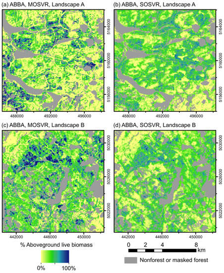
Figure 9.
Spatial predictions of relative abundance for species ABBA (balsam fir). Relative abundance predicted from (a,c) MOSVR and (b,d) SOSVR models, across two randomly positioned sample landscapes 12 km x 12 km in size (UTM zone 19N, WGS84). Masked areas include non-forest pixels, forest pixels affected by canopy change during the study period, or missing data due to cloud or snow cover. Predictions were truncated at 0 and 100%.
Whereas MOSVR predicted values up to 100%, SOSVR predictions infrequently exceeded 75%. The stronger attenuation bias of SOSVR generally suppressed local variability and produced a more uniform pattern of relative abundance than expected. MOSVR reduced attenuation bias, producing more realistic spatial patterns including patches of high relative abundance. These differences are important. Balsam fir is the primary host of the eastern spruce budworm (ESBW; Choristoneura fumiferana Clem.), a native insect that can cause widespread mortality of fir and spruce trees during cyclic outbreaks [65]. Vulnerability to ESBW defoliation is in large part determined by balsam fir relative abundance, with the greatest impact anticipated to occur in mature spruce-fir stands with fir relative abundance exceeding 75% [66]. Systematic under-estimation of vulnerability will ultimately cause underestimation of budworm impact. Additionally, because ESBW outbreak dynamics appear to be influenced by spatial distributions of host- and non-host-dominant stands [67,68], accurate predictions of tree species dominance and codominance should be important as well.
Finally, use of MOSVR presents certain challenges. Although the MATLAB implementation of NSGA-II provides an option for parallel execution, in our case the total execution time required for each species model ranged from 17–76 h, and averaged 46 h (using the MATLAB Parallel Computing Toolbox with 12 workers, one worker per physical CPU core, and a 3.40 GHz CPU). However, we did not systematically explore strategies to reduce execution time. Additionally, we recognize that outlier removal is a weakness of our current implementation. Further development is warranted, and we are investigating robust measures of systematic error as an alternative to outlier removal. Use of a GA for model training bears certain implications for model interpretation, particularly in a multi-objective framework. Similar performance characteristics may be achieved with different model specifications. Consequently, models lying near to one another on the Pareto front may show substantive differences in SVR parameters or variable/sample selections. MOSVR relative abundance models included on average 21 of 94 variables and excluded on average 24 samples from model training (Supplementary Table S2). For nearly all species, models included both spectral, terrain, and climatological variables. We caution against over-interpretation of variable selections and sample exclusions at this point, however, as GAs provide a group selection mechanism. Additional steps could be taken to evaluate the relative importance of variables. Post-hoc analyses of response and predictor variable values could be used to illuminate important relationships between variables (e.g., [69]). Inspection of variable selection and variable importance patterns across the Pareto front may provide insight into how certain variables influence attenuation. Similarly, further analysis of excluded samples might improve our understanding of whether and how certain plot or image conditions are more likely to affect levels of systematic error. This would require extensive analysis, however, since SVM model fit is determined by a subset of samples (SVs), and the selection or exclusion of a sample may or may not affect model fit under different parameter settings. All of these issues warrant further work.
5. Conclusions
Patterns of error observed in predictions of tree species relative abundance were consistent with strong attenuation bias caused by uncertainty in remote sensing and geospatial predictor data. Comparing results across different predictive models, systematic error as a fraction of total error was typically greatest in regression models that achieved the lowest total error. Pronounced underestimation at high relative abundance caused large deviations between predicted and observed patterns of species dominance and codominance. As expected, nearest neighbor methods produced better agreement with observed dominance/codominance by preserving observed species associations. Yet predictive accuracy was low and attenuation bias was high for individual species. Our multi-objective support vector regression (MOSVR) approach effectively reduced systematic error for all species while maintaining comparatively low total error, and improved predicted patterns of dominance/codominance to a level approaching that of the nearest neighbor methods.
Others have made compelling arguments that physical differences in scale and location between pixels and field plots are primary contributors to attenuation bias [7,8], and some have suggested that the use of FIA or similar forest inventory data for model training may be ill-advised [7,13]. Yet FIA data is often used to train predictive models, and although error patterns at the scale of predictions are not always reported (e.g., [5,70]), results are probably subject to some level of attenuation bias. Not all systematic error is indicative of model bias, but lacking detailed knowledge of predictor uncertainty and its impact in specific modeling frameworks, some level of correction is likely to be warranted. In that case, MOSVR can provide an effective machine learning approach to the reduction of systematic prediction error.
Supplementary Materials
The following are available online at https://www.mdpi.com/2072-4292/12/11/1739/s1, Table S1: Predictive performance by species and model type, Table S2: Multi-objective support vector regression variable selection, training sample selection, and influential outlier removal.
Author Contributions
Conceptualization, K.L. and E.S.-L.; Methodology, K.L. and E.S.-L.; Software, K.L.; Validation, K.L. and E.S.-L.; Formal Analysis, K.L., E.S.-L., and A.W.; Investigation, K.L. and E.S.-L.; Resources, A.W. and E.S.-L.; Data Curation, K.L. and E.S.-L.; Writing—Original Draft Preparation, K.L.; Writing—Review & Editing, K.L., E.S.-L., and A.W.; Visualization, K.L. and E.S.-L.; Supervision, K.L., E.S.-L., and A.W.; Project Administration, K.L., E.S.-L., and A.W.; Funding Acquisition, K.L., E.S.-L., and A.W. All authors have read and agreed to the published version of the manuscript.
Funding
This work was supported by the U.S. Carbon Cycle Science Program funded jointly by NASA and USDA National Institute of Food and Agriculture (2011-67003-30351), by the National Science Foundation Dynamics of Coupled Natural and Human Systems Program (DEB-1313688) and EPSCoR Program (RII-1920908), and by the Northeastern States Research Cooperative (projects entitled “Merging Landsat time-series and FIA data to develop vulnerability maps for spruce budworm decision support”, “Evaluating the interacting effects of forest management practices and periodic spruce budworm infestation on broad-scale, long-term forest productivity”, and “Long-term outcomes and tradeoffs of forest policy and management practices on the broad-scale sustainability of forest resources: wood supply, carbon, and wildlife habitat”).
Acknowledgments
Confidential coordinates of Forest Inventory and Analysis (FIA) field plots were made available through a collaborative agreement with the USDA Forest Service Northern Research Station FIA Program (FS Agreement No. 2014-MU-11242305-055). We thank Elizabeth Burrill for assistance in obtaining and working with FIA spatial data. We thank Steven Sader for supporting this work during its early conceptualization and development.
Conflicts of Interest
The authors declare no conflict of interest. The funders had no role in the design of the study; in the collection, analyses, or interpretation of data; in the writing of the manuscript, or in the decision to publish the results.
References
- Blackard, J.; Finco, M.; Helmer, E.; Holden, G.; Hoppus, M.; Jacobs, D.; Lister, A.; Moisen, G.G.; Nelson, M.; Riemann, R.; et al. forest biomass using nationwide forest inventory data and moderate resolution information. Remote Sens. Environ. 2008, 112, 1658–1677. [Google Scholar] [CrossRef]
- Powell, S.L.; Cohen, W.; Healey, S.P.; Kennedy, R.E.; Moisen, G.G.; Pierce, K.B.; Ohmann, J.L. Quantification of live aboveground forest biomass dynamics with Landsat time-series and field inventory data: A comparison of empirical modeling approaches. Remote Sens. Environ. 2010, 114, 1053–1068. [Google Scholar] [CrossRef]
- Pflugmacher, D.; Cohen, W.B.; Kennedy, R.E.; Yang, Z. Using Landsat-derived disturbance and recovery history and lidar to map forest biomass dynamics. Remote Sens. Environ. 2014, 151, 124–137. [Google Scholar] [CrossRef]
- Wolter, P.T.; Townsend, P.A.; Sturtevant, B.; Kingdon, C. Remote sensing of the distribution and abundance of host species for spruce budworm in Northern Minnesota and Ontario. Remote Sens. Environ. 2008, 112, 3971–3982. [Google Scholar] [CrossRef]
- Wilson, B.T.; Lister, A.J.; Riemann, R.I. A nearest-neighbor imputation approach to mapping tree species over large areas using forest inventory plots and moderate resolution raster data. For. Ecol. Manag. 2012, 271, 182–198. [Google Scholar] [CrossRef]
- Saatchi, S.; Marlier, M.; Chazdon, R.; Clark, D.B.; Russell, A.E. Impact of spatial variability of tropical forest structure on radar estimation of aboveground biomass. Remote Sens. Environ. 2011, 115, 2836–2849. [Google Scholar] [CrossRef]
- Xu, Y.; Dickson, B.G.; Hampton, H.M.; Sisk, T.D.; Palumbo, J.A.; Prather, J.W. Effects of Mismatches of Scale and Location between Predictor and Response Variables on Forest Structure Mapping. Photogramm. Eng. Remote Sens. 2009, 75, 313–322. [Google Scholar] [CrossRef]
- Réjou-Méchain, M.; Muller-Landau, H.C.; Detto, M.; Thomas, S.; le Toan, T.; Saatchi, S.S.; Barreto-Silva, J.S.; Bourg, N.A.; Bunyavejchewin, S.; Butt, N.; et al. Local spatial structure of forest biomass and its consequences for remote sensing of carbon stocks. Biogeosciences 2014, 11, 6827–6840. [Google Scholar] [CrossRef]
- McRoberts, R.E.; Bechtold, W.A.; Patterson, P.L.; Scott, C.T.; Reams, G.A. The Enhanced Forest Inventory and Analysis Program of the USDA Forest Service: Historical perspective and announcement of statistical documentation. J. For. 2005, 103, 304–308. [Google Scholar]
- Bartlett, J.; de Stavola, B.; Frost, C. Linear mixed models for replication data to efficiently allow for covariate measurement error. Stat. Med. 2009, 28, 3158–3178. [Google Scholar] [CrossRef]
- Frost, C.; Thompson, S.G. Correcting for regression dilution bias: Comparison of methods for a single predictor variable. J. R. Stat. Soc. Ser. A 2000, 163, 173–189. [Google Scholar] [CrossRef]
- Curran, P.J.; Hay, A. The importance of measurement error for certain procedures in remote sensing at optical wavelengths. Photogramm. Eng. Remote Sens. 1986, 52, 229–241. [Google Scholar]
- Robinson, C.; Saatchi, S.; Neumann, M.; Gillespie, T.W. Impacts of Spatial Variability on Aboveground Biomass Estimation from L-Band Radar in a Temperate Forest. Remote Sens. 2013, 5, 1001–1023. [Google Scholar] [CrossRef]
- Frescino, T.S.; Edwards, T.C.; Moisen, G.G. Modeling spatially explicit forest structural attributes using generalized additive models. J. Veg. Sci. 2001, 12, 15–26. [Google Scholar] [CrossRef]
- Ohmann, J.L.; Gregory, M.J.; Roberts, H. Scale considerations for integrating forest inventory plot data and satellite image data for regional forest mapping. Remote Sens. Environ. 2014, 151, 3–15. [Google Scholar] [CrossRef]
- Ohmann, J.L.; Gregory, M.J. Predictive mapping of forest composition and structure with direct gradient analysis and nearest neighbor imputation in coastal Oregon, USA Can. J. For. Res. 2002, 32, 725–741. [Google Scholar] [CrossRef]
- Riemann, R.; Wilson, B.T.; Lister, A.; Parks, S. An effective assessment protocol for continuous geospatial datasets of forest characteristics using USFS Forest Inventory and Analysis (FIA) data. Remote Sens. Environ. 2010, 114, 2337–2352. [Google Scholar] [CrossRef]
- Foster, S.D.; Shimadzu, H.; Darnell, R. Uncertainty in spatially predicted covariates: Is it ignorable? J. R. Stat. Soc. Ser. C 2012, 61, 637–652. [Google Scholar] [CrossRef]
- Denham, R.J.; Falk, M.G.; Mengersen, K. The Bayesian conditional independence model for measurement error: Applications in ecology. Environ. Ecol. Stat. 2010, 18, 239–255. [Google Scholar] [CrossRef][Green Version]
- McInerny, G.J.; Purves, D.W. Fine-scale environmental variation in species distribution modelling: Regression dilution, latent variables and neighbourly advice. Methods Ecol. Evol. 2011, 2, 248–257. [Google Scholar] [CrossRef]
- Mountrakis, G.; Im, J.; Ogole, C. Support vector machines in remote sensing: A review. ISPRS J. Photogramm. Remote Sens. 2011, 66, 247–259. [Google Scholar] [CrossRef]
- Salcedo-Sanz, S.; Rojo-Álvarez, J.L.; Martínez-Ramón, M.; Camps-Valls, G. Support vector machines in engineering: An overview. Wiley Interdiscip. Rev. Data Min. Knowl. Discov. 2014, 4, 234–267. [Google Scholar] [CrossRef]
- Yang, J.; Honavar, V.G. Feature subset selection using a genetic algorithm. IEEE Intell. Syst. 1998, 13, 44–49. [Google Scholar] [CrossRef]
- Blum, A.; Langley, P. Selection of relevant features and examples in machine learning. Artif. Intell. 1997, 97, 245–271. [Google Scholar] [CrossRef]
- Bazi, Y.; Melgani, F. Toward an Optimal SVM Classification System for Hyperspectral Remote Sensing Images. IEEE Trans. Geosci. Remote Sens. 2006, 44, 3374–3385. [Google Scholar] [CrossRef]
- Friedrichs, F.; Igel, C. Evolutionary tuning of multiple SVM parameters. Neurocomputing 2005, 64, 107–117. [Google Scholar] [CrossRef]
- Huang, C.-L.; Wang, C.-J. A GA-based feature selection and parameters optimization for support vector machines. Expert Syst. Appl. 2006, 31, 231–240. [Google Scholar] [CrossRef]
- Pasolli, L.; Notarnicola, C.; Bruzzone, L.; Bertoldi, G.; Della-Chiesa, S.; Niedrist, G.; Tappeiner, U.; Zebisch, M. Polarimetric Radarsat-2 imagery for soil moisture retrieval in alpine areas. Can. J. Remote Sens. 2012, 37, 535–547. [Google Scholar] [CrossRef]
- Goldberg, D.E. Genetic Algorithms in Search, Optimisation and Machine Learning; Addison-Wesley: New York, NY, USA, 1989. [Google Scholar]
- Konak, A.; Coit, D.W.; Smith, A.E. Multi-objective optimization using genetic algorithms: A tutorial. Reliab. Eng. Syst. Saf. 2006, 91, 992–1007. [Google Scholar] [CrossRef]
- Likens, G.E.; Franklin, J.F. Ecosystem thinking in the Northern Forest—And beyond. Bioscience 2009, 59, 511–513. [Google Scholar] [CrossRef][Green Version]
- Nightingale, J.M.; Fan, W.; Coops, N.C.; Waring, R. Predicting Tree Diversity Across the United States as a Function of Modeled Gross Primary Production. Ecol. Appl. 2008, 18, 93–103. [Google Scholar] [CrossRef] [PubMed]
- Seymour, R.S. The northeastern region. In Regional Silviculture of the United States; Barrett, J.W., Ed.; Wiley: New York, NY, USA, 1995; pp. 31–79. [Google Scholar]
- Smith, W.B. Forest inventory and analysis: A national inventory and monitoring program. Environ. Pollut. 2002, 116, 233–242. [Google Scholar] [CrossRef]
- O’Connell, B.; Conkling, B.L.; Wilson, A.M.; Burrill, E.A.; Turner, J.A.; Pugh, S.A.; Christiansen, G.; Ridley, T.; Menlove, J. The Forest Inventory and Analysis Database: Database Description and User Guide for Phase 2 (Version 6.1); U.S. Department of Agriculture, Forest Service: Asheville, NC, USA, 2016.
- Soenen, S.A.; Peddle, D.; Coburn, C. SCS+C: A modified Sun-canopy-sensor topographic correction in forested terrain. IEEE Trans. Geosci. Remote Sens. 2005, 43, 2148–2159. [Google Scholar] [CrossRef]
- Archuleta, C.-A.; Constance, E.W.; Arundel, S.T.; Lowe, A.J.; Mantey, K.S.; Phillips, L.A. The National Map seamless digital elevation model specifications. In Techniques and Methods; U.S. Geological Survey: Reston, VA, USA, 2017. [Google Scholar]
- Canty, M.J.; Nielsen, A.A. Automatic radiometric normalization of multitemporal satellite imagery with the iteratively re-weighted MAD transformation. Remote Sens. Environ. 2008, 112, 1025–1036. [Google Scholar] [CrossRef]
- Conrad, O.; Bechtel, B.; Bock, M.; Dietrich, H.; Fischer, E.; Gerlitz, L.; Wehberg, J.; Wichmann, V.; Böhner, J. System for Automated Geoscientific Analyses (SAGA) v. 2.1.4. Geosci. Model Dev. 2015, 8, 1991–2007. [Google Scholar] [CrossRef]
- Zevenbergen, L.W.; Thorne, C.R. Quantititaive analysis of land surface topography. Earth Surf. Process. Landf. 1987, 12, 47–56. [Google Scholar] [CrossRef]
- Ollinger, S.V.; Aber, J.D.; Federer, C.A.; Lovett, G.M.; Ellis, J.M. Modeling Physical and Chemical Climate of the Northeastern United States for a Geographic Information System; U.S. Department of Agriculture, Forest Service, Northern Research Station: Radnor, PA, USA, 1995.
- Quinn, P.; Beven, K.; Chevallier, P.; Planchon, O. The prediction of hillslope flow paths for distributed hydrological modelling using digital terrain models. Hydrol. Process. 1991, 5, 59–79. [Google Scholar] [CrossRef]
- Wang, L.; Liu, H. An efficient method for identifying and filling surface depressions in digital elevation models for hydrologic analysis and modelling. Int. J. Geogr. Inf. Sci. 2006, 20, 193–213. [Google Scholar] [CrossRef]
- Rehfeldt, G.E. A Spline Model of Climate for the Western United States; U.S. Department of Agriculture, Forest Service, Rocky Mountain Research Station: Fort Collins, CO, USA, 2006.
- Rehfeldt, G.E.; Crookston, N.L.; Warwell, M.V.; Evans, J. Empirical Analyses of Plant-Climate Relationships for the Western United States. Int. J. Plant Sci. 2006, 167, 1123–1150. [Google Scholar] [CrossRef]
- Beers, T.W.; Dress, P.E.; Wensel, L.C. Aspect transformation in site productivity research. J. For. 1966, 64, 691–692. [Google Scholar]
- Guisan, A.; Weiss, S.B. GLM versus CCA spatial modeling of plant species distribution. Plant Ecol. 1999, 143, 107–122. [Google Scholar] [CrossRef]
- Häntzschel, J.; Goldberg, V.; Bernhofer, C. GIS-based regionalisation of radiation, temperature and coupling measures in complex terrain for low mountain ranges. Meteorol. Appl. 2005, 12, 33–42. [Google Scholar] [CrossRef]
- Hepinstall, J.A.; Sader, S.A.; Krohn, W.B.; Boone, R.B.; Bartlett, R.I. Development and Testing of a Vegetation and Land Cover Map of Maine; Maine Agricultural and Forest Experiment Station, University of Maine: Orono, ME, USA, 1999. [Google Scholar]
- Brereton, R.; Lloyd, G.R. Support Vector Machines for classification and regression. Analyst 2010, 135, 230–267. [Google Scholar] [CrossRef] [PubMed]
- Deb, K.; Pratap, A.; Agarwal, S.; Meyarivan, T. A fast and elitist multiobjective genetic algorithm: NSGA-II. IEEE Trans. Evol. Comput. 2002, 6, 182–197. [Google Scholar] [CrossRef]
- Chang, C.-C.; Lin, C.-J. Libsvm: A library for support vector machines. ACM Trans. Intell. Syst. Technol. 2011, 2, 1–27. [Google Scholar] [CrossRef]
- Kim, J.-H. Estimating classification error rate: Repeated cross-validation, repeated hold-out and bootstrap. Comput. Stat. Data Anal. 2009, 53, 3735–3745. [Google Scholar] [CrossRef]
- Willmott, C. On the validation of models. Phys. Geogr. 1981, 2, 184–194. [Google Scholar] [CrossRef]
- Zäpfel, G.; Braune, R.; Bögl, M. Metaheuristic Search Concepts: A Tutorial with Applications to Production and Logistics; Springer: Heidelberg, Germany, 2010. [Google Scholar]
- Breiman, L. Random forests. Mach. Learn. 2001, 45, 5–32. [Google Scholar] [CrossRef]
- Crookston, N.L.; Finley, A.O. yaImpute: An R package for κNN imputation. J. Stat. Softw. 2008, 23, 1–16. [Google Scholar] [CrossRef]
- Hudak, A.T.; Crookston, N.L.; Evans, J.; Hall, D.; Falkowski, M.J. Nearest neighbor imputation of species-level, plot-scale forest structure attributes from LiDAR data. Remote Sens. Environ. 2008, 112, 2232–2245. [Google Scholar] [CrossRef]
- R Core Team. R: A Language and Environment for Statistical Computing; R Foundation for Statistical Computing. 2017. Available online: https://www.R.-project.org/ (accessed on 1 April 2020).
- Liaw, A.; Wiener, M. Classification, and regression by randomforest. R News 2002, 2, 18–22. [Google Scholar]
- Oksanen, J.; Blanchet, F.G.; Friendly, M.; Kindt, R.; Legendre, P.; McGlinn, D.; Minchin, P.R.; O’Hara, R.B.; Simpson, G.L.; Solymos, P.; et al. Vegan: Community Ecology Package; R Package Version 2.4-3. 2017. Available online: https://CRAN.R-project.org/package=vegan (accessed on 1 April 2020).
- Henderson, E.B.; Ohmann, J.L.; Gregory, M.J.; Roberts, H.; Zald, H.S. Species distribution modelling for plant communities: Stacked single species or multivariate modelling approaches? Appl. Veg. Sci. 2014, 17, 516–527. [Google Scholar] [CrossRef]
- Openshaw, S. The Modifiable Areal Unit Problem; GeoBooks: Norwich, UK, 1984. [Google Scholar]
- Carroll, R.J.; Ruppert, D.; Stefanski, L.A. Measurement Error in Nonlinear Models, Monographs on Statistics and Applied Probability 63; Chapman & Hall: London, UK, 1995. [Google Scholar]
- Morin, H.; Jardon, Y.; Gagnon, R. Relationship between spruce budworm outbreaks and forest dynamics in eastern North America. In Plant Disturbance Ecology: The Process and the Response; Johnson, E.A., Miyanishi, K., Eds.; Elsevier Science: Amsterdam, The Netherlands, 2007; pp. 555–577. [Google Scholar]
- Hennigar, C.R.; Wilson, J.S.; MacLean, D.A.; Wagner, R.G. Applying a spruce budworm decision support system to Maine: Projecting spruce-fir volume impacts under alternative management and outbreak scenarios. J. For. 2011, 109, 332–342. [Google Scholar]
- Bouchard, M.; Auger, I. Influence of environmental factors and spatio-temporal covariates during the initial development of a spruce budworm outbreak. Landsc. Ecol. 2013, 29, 111–126. [Google Scholar] [CrossRef]
- Campbell, E.M.; MacLean, D.A.; Bergeron, Y. The severity of budworm-caused growth reductions in balsam fir/spruce stands varies with the hardwood content of surrounding forest landscapes. For. Sci. 2008, 54, 195–205. [Google Scholar]
- Goldstein, A.; Kapelner, A.; Bleich, J.; Pitkin, E. Peeking Inside the Black Box: Visualizing Statistical Learning with Plots of Individual Conditional Expectation. J. Comput. Graph. Stat. 2015, 24, 44–65. [Google Scholar] [CrossRef]
- Duveneck, M.J.; Thompson, J.R.; Wilson, B.T. An imputed forest composition map for New England screened by species range boundaries. For. Ecol. Manag. 2015, 347, 107–115. [Google Scholar] [CrossRef]


© 2020 by the authors. Licensee MDPI, Basel, Switzerland. This article is an open access article distributed under the terms and conditions of the Creative Commons Attribution (CC BY) license (http://creativecommons.org/licenses/by/4.0/).