A Hybrid Approach Combining Conceptual Hydrological Models, Support Vector Machines and Remote Sensing Data for Rainfall-Runoff Modeling


Abstract
:1. Introduction
- How much do the intermediate variables obtained from the RR model correlate with in situ SM or remotely sensed SM products?
- Can the intermediate variables be effective in RR modeling within a machine learning-based regression framework, particularly for low flow simulations in a hybrid model?
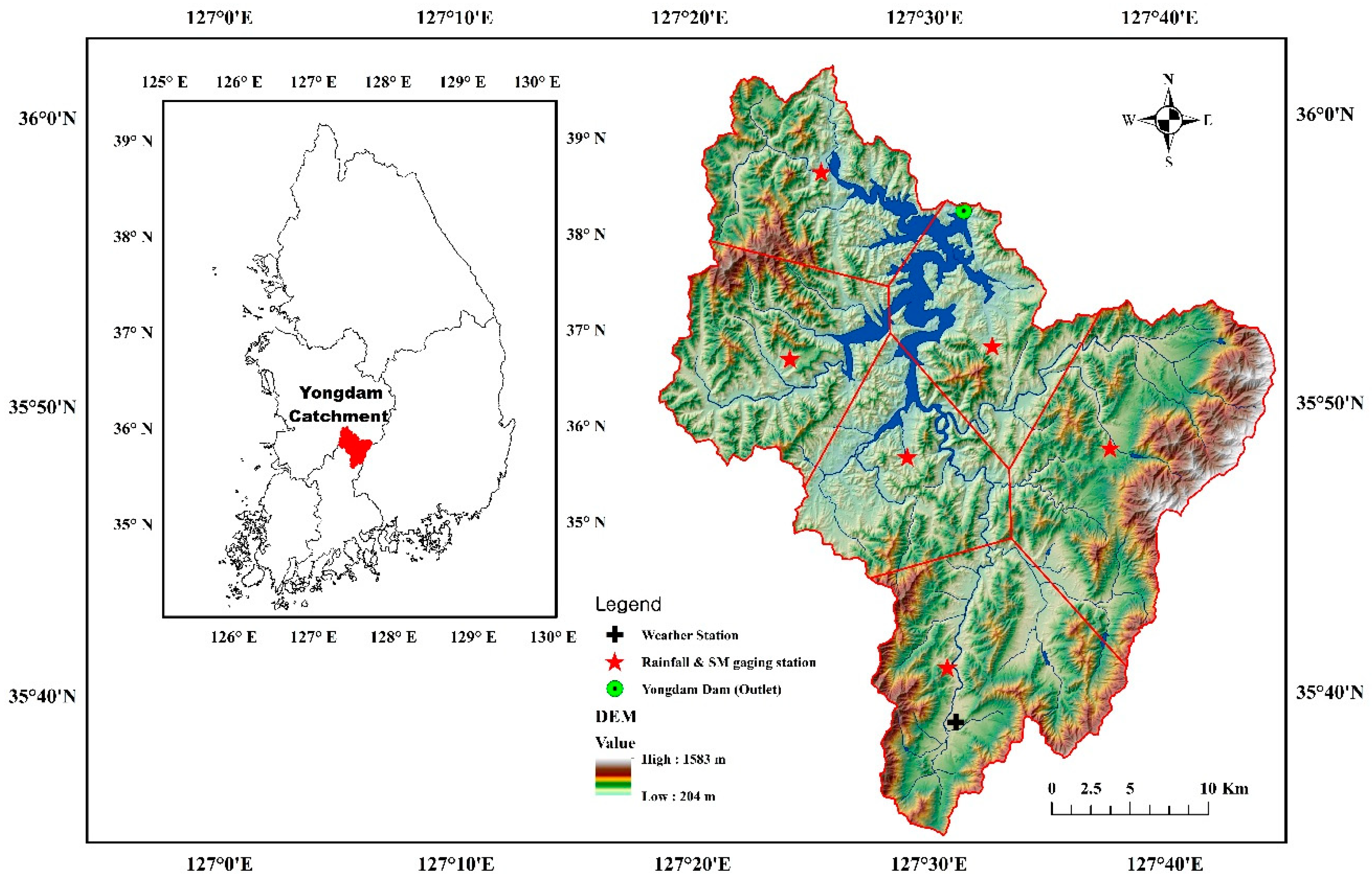
2. Study Area and Data
2.1. Study Area and In Situ Observations
2.2. Satellite SM Measurements
3. Methodology
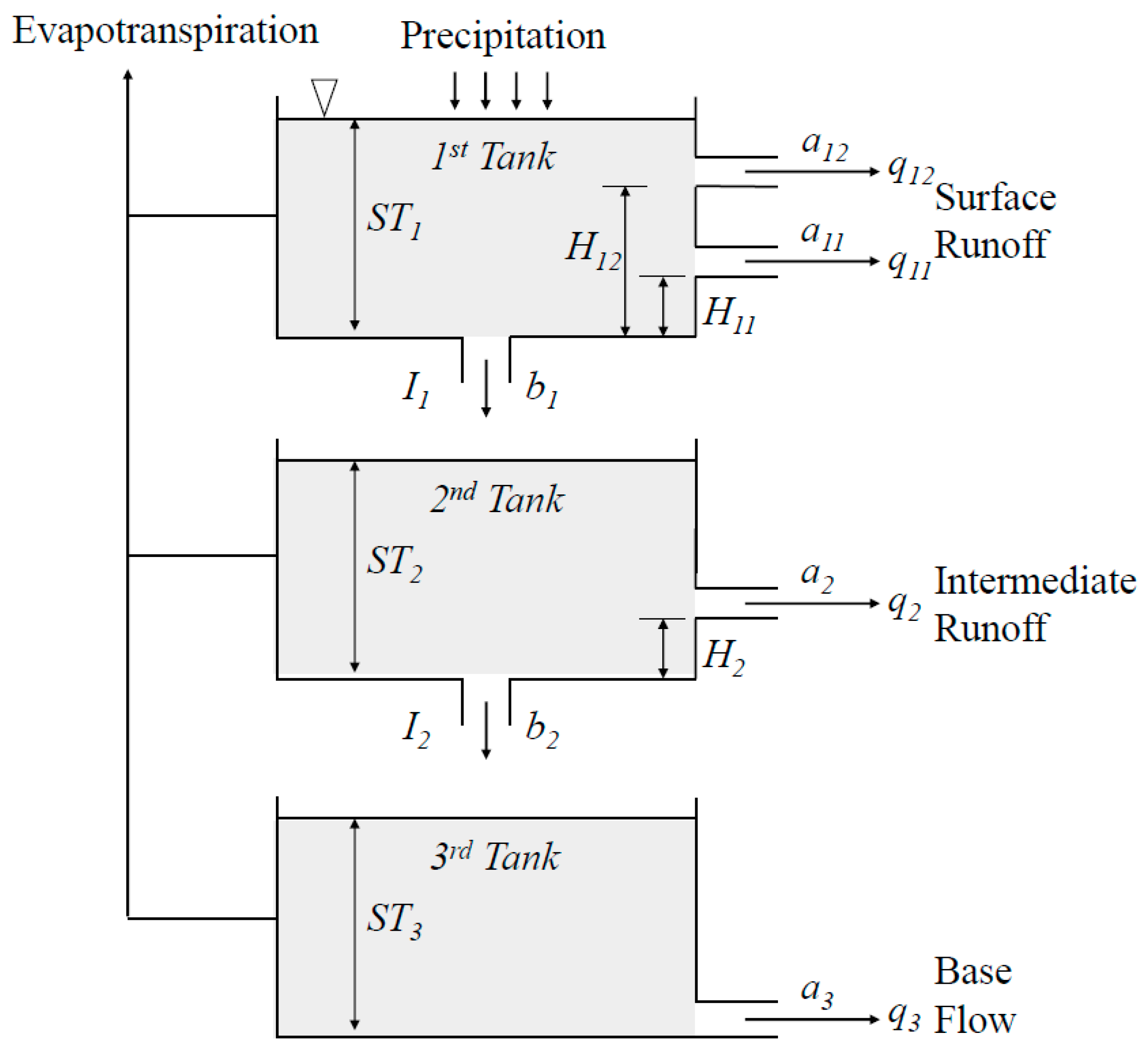
3.1. The Tank Model
3.2. The Least Square Support Vector Machine (LSSVM) Model
3.3. The Tank-LSSVM Hybrid Model
3.4. Root-Zone ESA CCI SM Products
3.5. Performance Scores
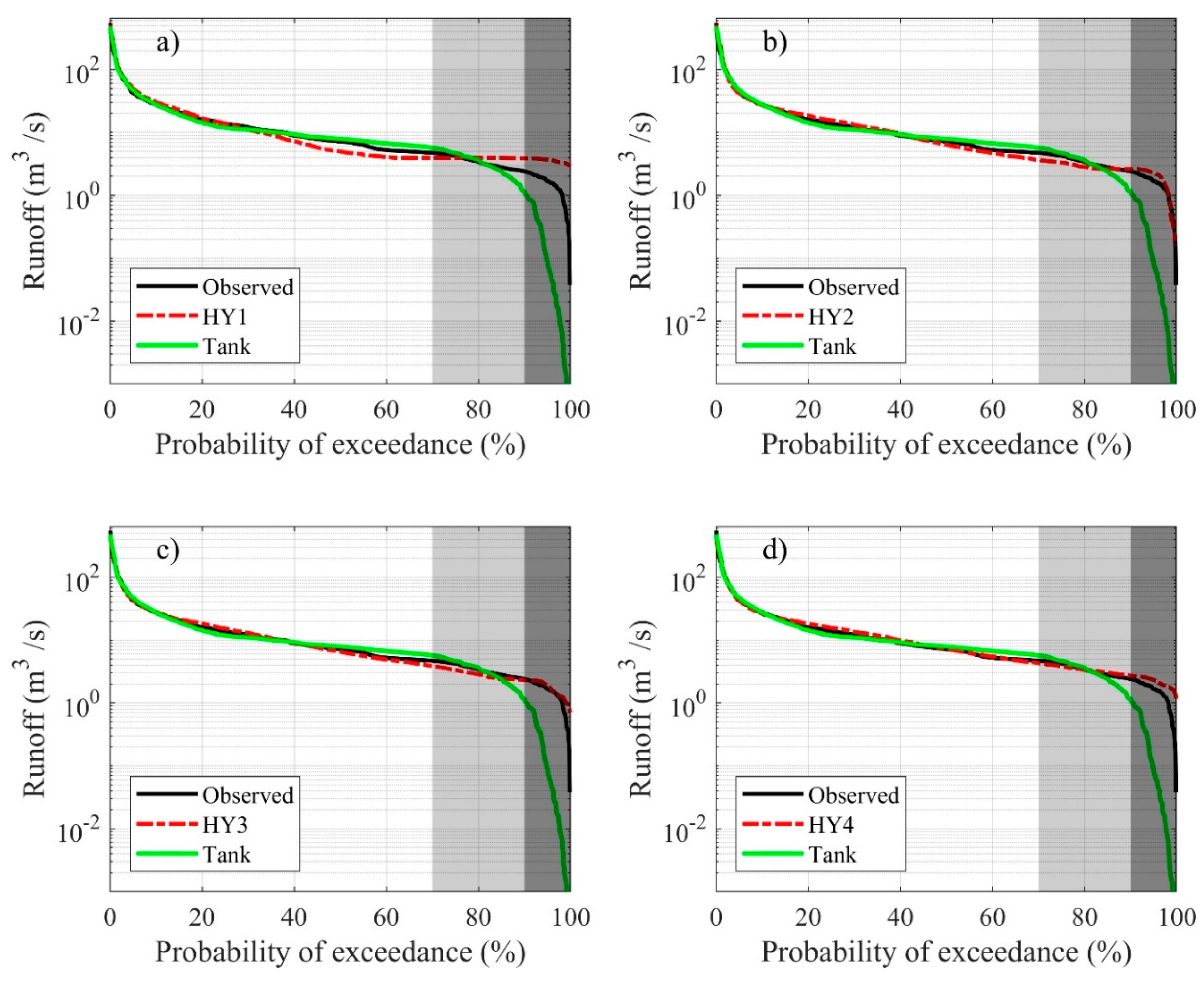
4. Results and Discussion
4.1. Rainfall-Runoff Using the Tank Model
4.2. LSSVM and Tank-LSSVM Models
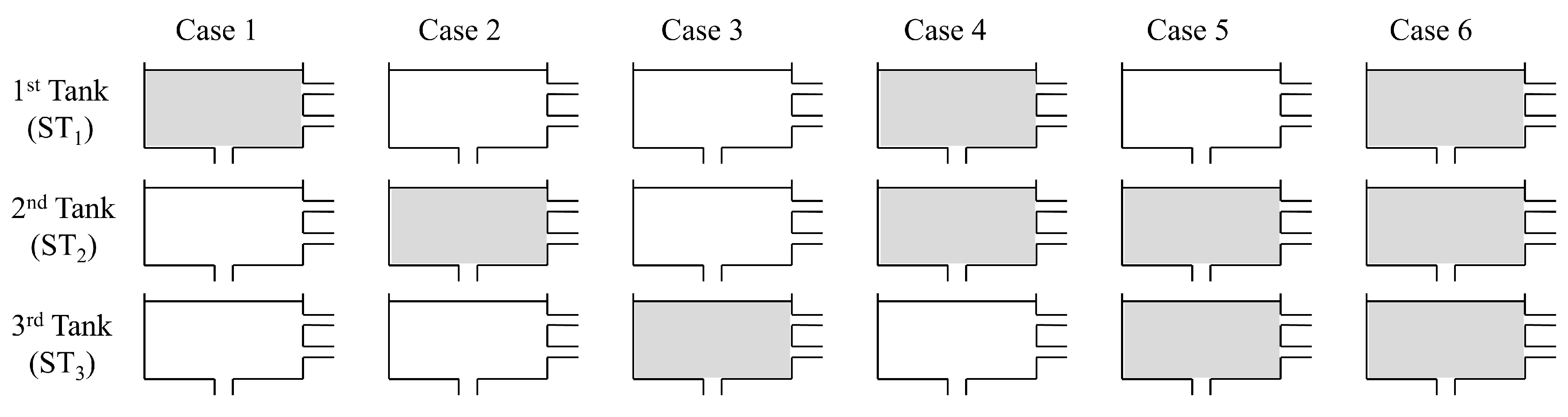
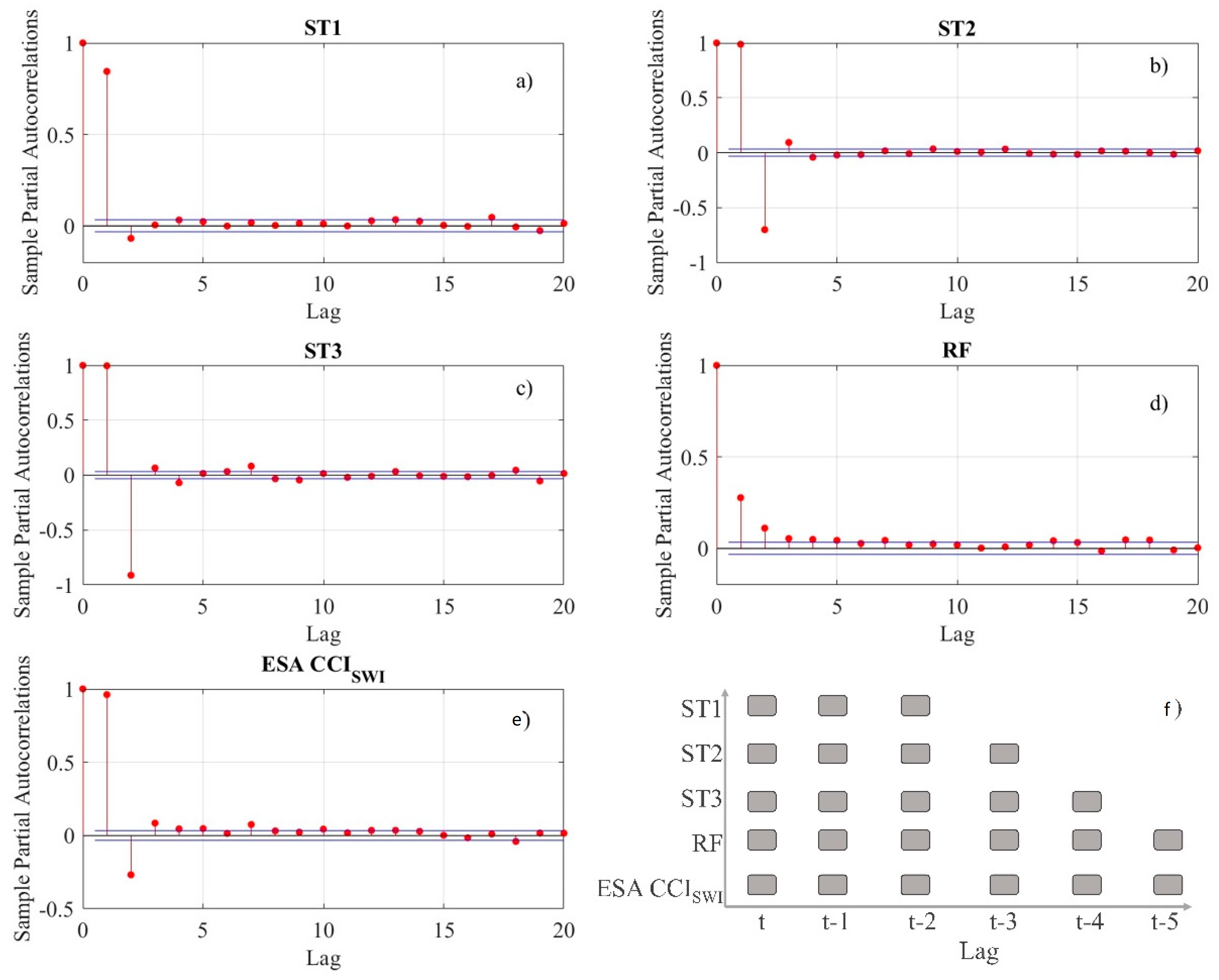
4.2.1. Determination of Model Inputs
4.2.2. LSSVM Model
4.2.3. Tank-LSSVM Model
5. Concluding Remarks
Author Contributions
Funding
Acknowledgments
Conflicts of Interest
Appendix A
References
- Curran, J.H. Streamflow Record Extension for Selected Strams in the Susitan River Basin, Alaska. US Geol. Surv. Sci. Investig. Rep 2012, 5210, 36. [Google Scholar]
- Sittner, W.T. WMO project on intercomparison of conceptual models used in hydrological forecasting. Hydrol. Sci. Bull. 1976, 21, 203–213. [Google Scholar] [CrossRef]
- Sivapragasam, C.; Liong, S.; Pasha, M. Rainfall and runoff forecasting with SSA-SVM approach. J. Hydroinform. 2001, 3, 141–152. [Google Scholar] [CrossRef] [Green Version]
- Zhuo, L.; Han, D. Could operational hydrological models be made compatible with satellite soil moisture observations? Hydrol. Process. 2016, 30, 1637–1648. [Google Scholar] [CrossRef] [Green Version]
- McIntyre, N.; Lee, H.; Wheater, H.; Young, A.; Wagener, T. Ensemble predictions of runoff in ungauged catchments. Water Resour. Res. 2005, 41, 1–14. [Google Scholar] [CrossRef] [Green Version]
- Jakeman, A.J. How Much Complexity Is Warranted in a Rainfall-Runoff Model? are good predictors of streamflow and. Water Resour. Res. 1993, 29, 2637–2649. [Google Scholar] [CrossRef]
- Pfannerstill, M.; Guse, B.; Fohrer, N. Smart low flow signature metrics for an improved overall performance evaluation of hydrological models. J. Hydrol. 2014, 510, 447–458. [Google Scholar] [CrossRef]
- Orth, R.; Staudinger, M.; Seneviratne, S.I.; Seibert, J.; Zappa, M. Does model performance improve with complexity? A case study with three hydrological models. J. Hydrol. 2015, 523, 147–159. [Google Scholar] [CrossRef] [Green Version]
- Kisi, O.; Parmar, K.S. Application of multivariate adaptive regression spline models in long term prediction of river water pollution. J. Hydrol. 2016, 534, 104–112. [Google Scholar] [CrossRef]
- Devia, G.K.; Ganasri, B.P.; Dwarakish, G.S. A Review on Hydrological Models. Aquat. Proced. 2015, 4, 1001–1007. [Google Scholar] [CrossRef]
- Behzad, M.; Asghari, K.; Eazi, M.; Palhang, M. Generalization performance of support vector machines and neural networks in runoff modeling. Expert Syst. Appl. 2009, 36, 7624–7629. [Google Scholar] [CrossRef]
- Young, C.C.; Liu, W.C.; Wu, M.C. A physically based and machine learning hybrid approach for accurate rainfall-runoff modeling during extreme typhoon events. Appl. Soft Comput. J. 2017, 53, 205–216. [Google Scholar] [CrossRef]
- Song, J.H.; Her, Y.; Park, J.; Lee, K.D.; Kang, M.S. Simulink Implementation of a Hydrologic Model: A Tank Model Case Study. Water 2017, 9, 639. [Google Scholar] [CrossRef] [Green Version]
- Paik, K.; Kim, J.H.; Kim, H.S.; Lee, D.R. A conceptual rainfall-runoff model considering seasonal variation. Hydrol. Process. 2005, 19, 475–476. [Google Scholar] [CrossRef]
- Beven, K.J.; Kirkby, M.J. A physically based, variable contributing area model of basin hydrology. Hydrol. Sci. Bull. 1979, 24, 43–69. [Google Scholar] [CrossRef] [Green Version]
- Burnash, R.J.; Ferral, R.L.; McGuire, R.A. A Generalized Streamflow Simulation System: Conceptual Models for Digital Computers; Joint Federal State River Forecast Center: Sacramento, CA, USA, 1973. [Google Scholar]
- Moore, R.J. The probability-distributed principle and runoff production at point and basin scales. Hydrol. Sci. J. 1985, 30, 273–297. [Google Scholar] [CrossRef] [Green Version]
- Bergström, S. Development and Application of a Conceptual Runoff Model for Scandinavian Catchments. Smhi 1976, RHO 7, 134. [Google Scholar] [CrossRef] [Green Version]
- Graham, D.N.; Butts, M.B. Flexible Integrated Watershed Modeling with MIKE SHE. In Watershed Models; Singh, V.P., Donald, K.F., Eds.; CRC Press: Boca Raton, FL, USA, 2005; pp. 245–272. ISBN 0849336090. [Google Scholar]
- Neitsch, S.; Arnold, J.; Kiniry, J.; Williams, J. Soil and Water Assessment Tool Theoretical Documentation Version 2009; Texas Water Resources Institute: College Station, TX, USA, 2011. [Google Scholar]
- Vaze, J.; Jordan, P.; Beecham, R.; Frost, A.; Summerell, G. Guidelines for Rainfall-Runoff Modelling: Towards Best Practice Model Application; eWater Cooprative Research Centre: Australia, 2011; ISBN 9781921543517. [Google Scholar]
- Sugawara, M. Automatic calibration of the tank model. Hydrol. Sci. Bull. 1979, 24, 375–388. [Google Scholar] [CrossRef]
- Basri, H. Development of Rainfall-runoff Model Using Tank Model: Problems and Challenges in Province of Aceh, Indonesia. Aceh Int. J. Sci. Technol. 2013, 2, 26–36. [Google Scholar] [CrossRef]
- Fumikazu, N.; Toshisuke, M.; Yoshio, H.; Hiroshi, T.; Kimihito, N. Evaluation of water resources by snow storage using water balance and tank model method in the Tedori River basin of Japan. Paddy Water Environ. 2013, 11, 113–121. [Google Scholar] [CrossRef]
- Samui, P.; Kothari, D.P. Utilization of a least square support vector machine (LSSVM) for slope stability analysis. Sci. Iran. 2011, 18, 53–58. [Google Scholar] [CrossRef] [Green Version]
- Bray, M.; Han, D. Identification of support vector machines for runoff modelling. J. Hydroinform. 2004, 265–280. [Google Scholar] [CrossRef] [Green Version]
- Granata, F.; Gargano, R.; de Marinis, G. Support Vector Regression for Rainfall-Runoff Modeling in Urban Drainage: A Comparison with the EPA’s Storm Water Management Model. Water 2016, 8, 69. [Google Scholar] [CrossRef]
- Wu, M.C.; Lin, G.F.; Lin, H.Y. Improving the forecasts of extreme streamflow by support vector regression with the data extracted by self-organizing map. Hydrol. Process. 2014, 28, 386–397. [Google Scholar] [CrossRef]
- Fernando, A.K.; Shamseldin, A.Y.; Abrahart, R.J. Use of Gene Expression Programming for Multimodel Combination of Rainfall-Runoff Models. J. Hydrol. Eng. 2012, 17, 975–985. [Google Scholar] [CrossRef] [Green Version]
- Hosseini, S.M.; Mahjouri, N. Integrating Support Vector Regression and a geomorphologic Artificial Neural Network for daily rainfall-runoff modeling. Appl. Soft Comput. J. 2016, 38, 329–345. [Google Scholar] [CrossRef]
- Okkan, U.; Serbes, Z.A. Rainfall-runoff modeling using least squares support vector machines. Environmetrics 2012, 23, 549–564. [Google Scholar] [CrossRef]
- Massari, C.; Brocca, L.; Ciabatta, L.; Moramarco, T.; Gabellani, S.; Albergel, C.; De Rosnay, P.; Puca, S.; Wagner, W. The Use of H-SAF Soil Moisture Products for Operational Hydrology: Flood Modelling over Italy. Hydrology 2015, 2, 2–22. [Google Scholar] [CrossRef] [Green Version]
- Dorigo, W.; Wagner, W.; Albergel, C.; Albrecht, F.; Balsamo, G.; Brocca, L.; Chung, D.; Ertl, M.; Forkel, M.; Gruber, A.; et al. ESA CCI Soil Moisture for improved Earth system understanding: State-of-the art and future directions. Remote Sens. Environ. 2017, 203, 185–215. [Google Scholar] [CrossRef]
- Loizu, J.; Massari, C.; Álvarez-Mozos, J.; Tarpanelli, A.; Brocca, L.; Casalí, J. On the assimilation set-up of ASCAT soil moisture data for improving streamflow catchment simulation. Adv. Water Resour. 2018, 111, 86–104. [Google Scholar] [CrossRef]
- Brocca, L.; Melone, F.; Moramarco, T.; Wager, W.; Naeimi, V.; Bartalis, Z.; Hasenauer, S. Improving runoff prediction through the assimilation of the ASCAT soil moisture product. Hydrol. Earth Syst. Sci. 2010, 14, 1881–1893. [Google Scholar] [CrossRef] [Green Version]
- Dharssi, I.; Bovis, K.J.; Macpherson, B.; Jones, C.P. Operational assimilation of ASCAT surface soil wetness at the Met Office. Hydrol. Earth Syst. Sci. 2011, 15, 2729–2746. [Google Scholar] [CrossRef] [Green Version]
- Ciabatta, L.; Massari, C.; Brocca, L.; Gruber, A.; Reimer, C.; Hahn, S.; Paulik, C.; Dorigo, W.; Kidd, R.; Wagner, W. SM2RAIN-CCI: A new global long-term rainfall data set derived from ESA CCI soil moisture. Earth Syst. Sci. Data 2018, 10, 267–280. [Google Scholar] [CrossRef] [Green Version]
- Brocca, L.; Ciabatta, L.; Massari, C.; Moramarco, T.; Hahn, S.; Hasenauer, S.; Kidd, R.; Dorigo, W.; Wagner, W.; Levizzani, V. Journal of Geophysical Research: Atmospheres rainfall from satellite soil moisture data. J. Geophys. Res. 2014, 1–14. [Google Scholar] [CrossRef]
- Enenkel, M.; Steiner, C.; Mistelbauer, T.; Dorigo, W.; Wagner, W.; See, L.; Atzberger, C.; Schneider, S.; Rogenhofer, E. A combined satellite-derived drought indicator to support humanitarian aid organizations. Remote Sens. 2016, 8, 340. [Google Scholar] [CrossRef] [Green Version]
- Brocca, L.; Moramarco, T.; Melone, F.; Wagner, W.; Hasenauer, S.; Hahn, S. Assimilation of surface- and root-zone ASCAT soil moisture products into rainfall-runoff modeling. IEEE Trans. Geosci. Remote Sens. 2012, 50, 2542–2555. [Google Scholar] [CrossRef]
- Lievens, H.; Tomer, S.K.; Al Bitar, A.; De Lannoy, G.J.M.; Drusch, M.; Dumedah, G.; Hendricks Franssen, H.J.; Kerr, Y.H.; Martens, B.; Pan, M.; et al. SMOS soil moisture assimilation for improved hydrologic simulation in the Murray Darling Basin, Australia. Remote Sens. Environ. 2015, 168, 146–162. [Google Scholar] [CrossRef]
- Massari, C.; Brocca, L.; Tarpanelli, A.; Moramarco, T. Data assimilation of satellite soil moisture into rainfall-runoffmodelling: A complex recipe? Remote Sens. 2015, 7, 11403–11433. [Google Scholar] [CrossRef] [Green Version]
- Han, E.; Merwade, V.; Heathman, G.C. Implementation of surface soil moisture data assimilation with watershed scale distributed hydrological model. J. Hydrol. 2012, 416–417, 98–117. [Google Scholar] [CrossRef]
- Yoo, J.H. Maximization of hydropower generation through the application of a linear programming model. J. Hydrol. 2009, 376, 182–187. [Google Scholar] [CrossRef]
- Topp, G.C.; Davis, J.L.; Annan, A.P. Electromagnetic Determination of Soil Water Content: Measruements in Coaxial Transmission Lines. Water Resour. Res. 1980, 16, 574–582. [Google Scholar] [CrossRef] [Green Version]
- Dorigo, W.A.; Gruber, A.; De Jeu, R.A.M.; Wagner, W.; Stacke, T.; Loew, A.; Albergel, C.; Brocca, L.; Chung, D.; Parinussa, R.M.; et al. Evaluation of the ESA CCI soil moisture product using ground-based observations. Remote Sens. Environ. 2015, 162, 380–395. [Google Scholar] [CrossRef]
- Liu, Y.Y.; Dorigo, W.A.; Parinussa, R.M.; De Jeu, R.A.M.; Wagner, W.; McCabe, M.F.; Evans, J.P.; Van Dijk, A.I.J.M. Trend-preserving blending of passive and active microwave soil moisture retrievals. Remote Sens. Environ. 2012, 123, 280–297. [Google Scholar] [CrossRef]
- Liu, Y.Y.; Parinussa, R.M.; Dorigo, W.A.; De Jeu, R.A.M.; Wagner, W.; Van Dijk, M.A.I.J.; McCabe, M.F.; Evans, J.P. Developing an improved soil moisture dataset by blending passive and active microwave satellite-based retrievals. Hydrol. Earth Syst. Sci. 2011, 15, 425–436. [Google Scholar] [CrossRef] [Green Version]
- Allen, R.G.; Pereira, L.S.; Raes, D.; Smith, M.; Ab, W. Crop Evapotranspiration—Guidelines for Computing Reference Crop Evapotranspiration; FAO: Roma, Italy, 1998; pp. 1–15. [Google Scholar]
- Vapnik, V. The Nature of Statistical Learning Theory; Springer: New York, NY, USA, 1995. [Google Scholar]
- Raghavendra, S.; Deka, P.C. Support vector machine applications in the field of hydrology: A review. Appl. Soft Comput. J. 2014, 19, 372–386. [Google Scholar] [CrossRef]
- Yan, X.; Chowdhury, N.A. Mid-term electricity market clearing price forecasting: A hybrid LSSVM and ARMAX approach. Int. J. Electr. Power Energy Syst. 2013, 53, 20–26. [Google Scholar] [CrossRef]
- Suykens, J.A.K.; De Brabanter, J.; Lukas, L.; Vandewalle, J. Weighted least squares support vector machines: Robustness and sparce approximation. Neurocomputing 2002, 48, 85–105. [Google Scholar] [CrossRef]
- Xavier-De-Souza, S.; Suykens, J.A.K.; Vandewalle, J.; Bolle, D. Coupled simulated annealing. IEEE Trans. Syst. Man Cybern. Part B Cybern. 2010, 40, 320–335. [Google Scholar] [CrossRef]
- Nelder, J.A.; Mead, R. A Simplex Method for Function Minimization. Comput. J. 1965, 7, 308–313. [Google Scholar] [CrossRef]
- Yu, P.S.; Chen, S.T.; Chang, I.F. Support vector regression for real-time flood stage forecasting. J. Hydrol. 2006, 328, 704–716. [Google Scholar] [CrossRef]
- Massari, C.; Brocca, L.; Barbetta, S.; Papathanasiou, C.; Mimikou, M.; Moramarco, T. Using globally available soil moisture indicators for flood modelling in Mediterranean catchments. Hydrol. Earth Syst. Sci. 2014, 18, 839–853. [Google Scholar] [CrossRef] [Green Version]
- Massari, C.; Camici, S.; Ciabatta, L.; Brocca, L. Exploiting satellite-based surface soil moisture for flood forecasting in the Mediterranean area: State update versus rainfall correction. Remote Sens. 2018, 10, 292. [Google Scholar] [CrossRef] [Green Version]
- Silvestro, F.; Gabellani, S.; Rudari, R.; Delogu, F.; Laiolo, P.; Boni, G. Uncertainty reduction and parameter estimation of a distributed hydrological model with ground and remote-sensing data. Hydrol. Earth Syst. Sci. 2015, 19, 1727–1751. [Google Scholar] [CrossRef] [Green Version]
- Albergel, C.; Rüdiger, C.; Pellarin, T.; Calvet, J.-C.; Fritz, N.; Froissard, F.; Suquia, D.; Petitpa, A.; Piguet, B.; Martin, E. From near-surface to root-zone soil moisture using an exponential filter: An assessment of the method based on in-situ observations and model simulations. Hydrol. Earth Syst. Sci. Discuss. 2008, 5, 1603–1640. [Google Scholar] [CrossRef] [Green Version]
- Wagner, W.; Lemoine, G.; Rott, H. A method for estimating soil moisture from ERS Scatterometer and soil data. Remote Sens. Environ. 1999, 70, 191–207. [Google Scholar] [CrossRef]
- Legates, D.R.; McCabe, G.J. Evaluating the use of “goodness-of-fit” measures in hydrologic and hydroclimatic model validation. Water Resour. Res. 1999, 35, 233–241. [Google Scholar] [CrossRef]
- Kalin, L.; Isik, S.; Schoonover, J.E.; Lockaby, B.G. Predicting Water Quality in Unmonitored Watersheds Using Artificial Neural Networks. J. Environ. Qual. 2010, 39, 1429. [Google Scholar] [CrossRef]
- Bober, W. Introduction to Numerical and Analytical Methods with MATLAB for Engineers and Scientists; CRC Press: Boca Raton, FL, USA, 2013; ISBN 9781466576094. [Google Scholar]


| Performance Metrics | Equations | Range | Optimal Value |
|---|---|---|---|
| Nash–Sutcliffe efficiency (NSE) | −∞~1 | 1 | |
| Coefficient of determination () | 0~1 | 1 | |
| Root mean square error (RMSE) | 0~∞ | 0 |
| Parameter | a11 | a12 | a20 | a30 | b1 | b2 | b3 | h11 | h12 | h20 | |
|---|---|---|---|---|---|---|---|---|---|---|---|
| Range | Min. | 0.08 | 0.08 | 0.03 | 0.00 | 0.10 | 0.01 | 0.00 | 5.00 | 20.00 | 0.00 |
| Max. | 0.50 | 1.00 | 1.00 | 0.03 | 0.50 | 0.35 | 0.11 | 60.00 | 150.00 | 100.00 | |
| Obtained value | 0.13 | 0.33 | 0.71 | 0.02 | 0.14 | 0.07 | 0.01 | 10.72 | 62.94 | 35.14 | |
| Model | Input Combinations | Training (2007–2013) | Testing (2014–2016) | ||||||
|---|---|---|---|---|---|---|---|---|---|
| NSE | RMSE | RMSE Q70 | NSE | RMSE | RMSE Q70 | ||||
| SV1 | P(t) | 0.60 | 0.60 | 44.72 | 10.40 | 0.40 | 0.49 | 26.02 | 9.86 |
| SV2 | P(t), (t−1) | 0.84 | 0.84 | 28.21 | 6.73 | 0.45 | 0.61 | 24.81 | 5.42 |
| SV3 | P(t), …, P(t−2) | 0.88 | 0.88 | 24.88 | 5.11 | 0.57 | 0.65 | 22.04 | 4.49 |
| SV4 | P(t), …, P(t−3) | 0.89 | 0.89 | 23.01 | 4.44 | 0.62 | 0.70 | 20.77 | 3.99 |
| SV5 | P(t), …, P(t−4) | 0.91 | 0.91 | 21.33 | 4.00 | 0.68 | 0.75 | 18.91 | 3.86 |
| SV6 | P(t), …, P(t−4), (t) | 0.91 | 0.91 | 21.24 | 3.18 | 0.69 | 0.77 | 18.80 | 4.79 |
| SV7 | P(t), …, P(t−4), (t), (t−1) | 0.91 | 0.91 | 20.74 | 3.29 | 0.69 | 0.77 | 18.62 | 5.02 |
| SV8 | P(t), …, P(t−4), (t), …, (t−2) | 0.92 | 0.92 | 19.53 | 3.12 | 0.72 | 0.79 | 17.90 | 4.93 |
| SV9 | P(t), …, P(t−4), (t), …, (t−3) | 0.92 | 0.92 | 19.33 | 2.98 | 0.73 | 0.81 | 17.51 | 4.75 |
| Model | Input Combinations | Training (2007–2013) | Testing (2014–2016) | ||||||
|---|---|---|---|---|---|---|---|---|---|
| NSE | RMSE | RMSE Q70 | NSE | RMSE | RMSE Q70 | ||||
| Tank | 0.92 | 0.96 | 20.18 | 3.74 | 0.81 | 0.91 | 14.72 | 3.12 | |
| HY1 | P(t), ST1(t) | 0.92 | 0.96 | 19.74 | 4.19 | 0.75 | 0.80 | 16.63 | 3.11 |
| HY2 | P(t), ST1(t), ST2(t) | 0.93 | 0.96 | 18.49 | 2.99 | 0.76 | 0.80 | 16.52 | 2.67 |
| HY3 | P(t), ST1(t), ST2(t), ST3(t) | 0.95 | 0.97 | 16.24 | 2.50 | 0.85 | 0.86 | 12.91 | 2.13 |
| HY4 | P(t), ST1(t), ST2(t), ST3(t), (t) | 0.94 | 0.97 | 17.43 | 2.34 | 0.85 | 0.85 | 12.96 | 2.23 |
| HY5 | P(t), P(t−1), ST1(t) | 0.92 | 0.96 | 19.87 | 4.40 | 0.71 | 0.77 | 17.93 | 3.11 |
| HY6 | P(t), ST1(t), ST1(t−1), ST2(t), ST3(t) | 0.93 | 0.96 | 18.75 | 2.94 | 0.84 | 0.85 | 13.38 | 2.19 |
| HY7 | P(t), ST1(t), ST2(t), ST2(t−1), ST3(t) | 0.93 | 0.96 | 18.87 | 2.99 | 0.85 | 0.85 | 13.18 | 2.34 |
| HY8 | P(t), ST1(t), ST2(t), ST3(t), ST3(t−1) | 0.93 | 0.96 | 18.97 | 2.93 | 0.85 | 0.85 | 13.13 | 2.39 |
| HY9 | P(t), ST1(t), ST2(t), ST3(t), (t), (t−1) | 0.93 | 0.96 | 18.98 | 2.81 | 0.85 | 0.85 | 13.14 | 2.49 |
© 2020 by the authors. Licensee MDPI, Basel, Switzerland. This article is an open access article distributed under the terms and conditions of the Creative Commons Attribution (CC BY) license (http://creativecommons.org/licenses/by/4.0/).
Share and Cite
Kwon, M.; Kwon, H.-H.; Han, D. A Hybrid Approach Combining Conceptual Hydrological Models, Support Vector Machines and Remote Sensing Data for Rainfall-Runoff Modeling. Remote Sens. 2020, 12, 1801. https://doi.org/10.3390/rs12111801
Kwon M, Kwon H-H, Han D. A Hybrid Approach Combining Conceptual Hydrological Models, Support Vector Machines and Remote Sensing Data for Rainfall-Runoff Modeling. Remote Sensing. 2020; 12(11):1801. https://doi.org/10.3390/rs12111801
Chicago/Turabian StyleKwon, Moonhyuk, Hyun-Han Kwon, and Dawei Han. 2020. "A Hybrid Approach Combining Conceptual Hydrological Models, Support Vector Machines and Remote Sensing Data for Rainfall-Runoff Modeling" Remote Sensing 12, no. 11: 1801. https://doi.org/10.3390/rs12111801