Modelling Crop Biomass from Synthetic Remote Sensing Time Series: Example for the DEMMIN Test Site, Germany

Abstract

This study compares the performance of the five widely used crop growth models (CGMs): World Food Studies (WOFOST), Coalition for Environmentally Responsible Economies (CERES)-Wheat, AquaCrop, cropping systems simulation model (CropSyst), and the semi-empiric light use efficiency approach (LUE) for the prediction of winter wheat biomass on the Durable Environmental Multidisciplinary Monitoring Information Network (DEMMIN) test site, Germany. The study focuses on the use of remote sensing (RS) data, acquired in 2015, in CGMs, as they offer spatial information on the actual conditions of the vegetation. Along with this, the study investigates the data fusion of Landsat (30 m) and Moderate Resolution Imaging Spectroradiometer (MODIS) (500 m) data using the spatial and temporal reflectance adaptive reflectance fusion model (STARFM) fusion algorithm. These synthetic RS data offer a 30-m spatial and one-day temporal resolution. The dataset therefore provides the necessary information to run CGMs and it is possible to examine the fine-scale spatial and temporal changes in crop phenology for specific fields, or sub sections of them, and to monitor crop growth daily, considering the impact of daily climate variability. The analysis includes a detailed comparison of the simulated and measured crop biomass. The modelled crop biomass using synthetic RS data is compared to the model outputs using the original MODIS time series as well. On comparison with the MODIS product, the study finds the performance of CGMs more reliable, precise, and significant with synthetic time series. Using synthetic RS data, the models AquaCrop and LUE, in contrast to other models, simulate the winter wheat biomass best, with an output of high R² (>0.82), low RMSE (<600 g/m²) and significant p-value (<0.05) during the study period. However, inputting MODIS data makes the models underperform, with low R² (<0.68) and high RMSE (>600 g/m²). The study shows that the models requiring fewer input parameters (AquaCrop and LUE) to simulate crop biomass are highly applicable and precise. At the same time, they are easier to implement than models, which need more input parameters (WOFOST and CERES-Wheat).

1. Introduction

The contention to achieve food security and the sustainable use of agricultural resources becomes vital due to the growth in the human population [1]. The World Summit on Food Security states that the community expects to reach a margin of 10 billion by 2050, and this will force intensive agriculture demand, along with the biggest challenge of climate change [2,3]. In this context, achieving sustainability in agriculture might slow down the negative impacts on the quantity and quality of soil and water resources, land degradation, greenhouse emissions, or biodiversity [4].

For the implementation of sustainable activities in agriculture, there is a definite requirement of monitoring crop growth and status in different regions and environmental contexts, with high temporal resolutions [5]. Efficient methodologies that are both able to monitor crop conditions and changing weather conditions near real-time are essential [1]. Also, these methodologies can be applied to predict crop production, e.g., for optimizing the management strategies in agriculture and increasing sustainability [6]. These crop predictions are not only essential to obtain the economic returns, but are, at the same time, highly valuable to efficiently evaluate food production insufficiency and to ensure food security in the agricultural regions of the world [7].

In the last two decades, crop growth models (CGMs) have reached a high degree of success in simulating the behavior of real crops (i.e., by predicting its final state of total biomass or harvestable yield). CGMs are defined as a set of mathematical equations which provide quantitative and temporal information on plant growth and development by including the effect of various climatic parameters [8]. These models, working on different spatial scales, are increasingly applied as tools for decision-making and research, e.g., they are used in plant management in order to evaluate climate risks [9,10]. On the contrary, CGMs lack the spatial information to estimate yield at the field scale [11]. Regulating model inputs for the required spatial and temporal scales is complicated, and the frequently assumed spatial homogeneity of crucial input parameters leads to errors in the estimated outputs [12,13]. A synergistic approach, linking remote sensing (RS) data with crop growth modeling, has the potential to overcome these limitations, as satellite RS offers a method to examine the fine-scale spatial and temporal changes in crop phenology for specific fields and to forecast crop yields, considering the impact of daily climate variability [14]. The integration of RS data into CGMs provides the practical information of the crop’s lifecycle by adjusting model parameters based on RS observations. Many studies successfully utilized the leaf area index (LAI), or fraction of absorbed photosynthetic active radiation (FPAR) derived from vegetation indices, e.g., the normalized difference vegetation index (NDVI), in combination with CGMs to estimate crop biomass or yield at different study regions around the world [11,15,16,17,18].

Due to economic accessibility, historical records and increasing resolutions of globally available satellite products now provide a new level of data with high spatial, temporal, and spectral resolutions, which in turn creates new possibilities for generating accurate datasets on several crop types and their respective yields [19,20,21]. Specifically for agricultural related applications, such as precision farming, field level information (a few tens of meters) is needed to guide farmers, while swift and subtle changes in crop conditions due to extreme weather events require the capture of high frequency images (i.e., daily or weekly acquisitions) [22,23]. The Landsat mission, which has provided optical multi-spectral RS data since the 1980s with 30m spatial resolution, is exemplary. However, Landsat satellites have a rather low temporal resolution with a revisit time of 16 days, and a high cloud coverage [24,25], which does not allow for crop phenology estimation on a daily or even weekly basis. Other RS systems, on the other hand, have a daily revisit but suffer from rather coarse spatial resolution, e.g., the Moderate Resolution Imaging Spectroradiometer (MODIS) imagery has provided multi-spectral RS data with a daily revisit since 2001. Due to its high frequency, spatial and temporal filtering methods are used to eliminate cloud-contaminated pixels with a high accuracy [26,27,28,29]; however, the effectiveness for fine-scale environmental applications is rather low and limited by the spatial resolution of 250 to 1000 m [30].

One way to overcome this issue is the application of multi-temporal data fusion. In such a fusion, two data sets are combined to create a synthetic time series, delivering both high spatial and high temporal resolution [31]. An example is the fusion of Landsat and MODIS imagery, creating a synthetic, consistent, and continues daily time series with a 30 m spatial resolution. Recently, many studies have applied different algorithms to fuse coarse and high-resolution imagery in the application of vegetation monitoring (e.g., [32,33]). The rise in the development of the usage of fusion algorithms is due to their higher spatial, temporal, and spectral resolution, with an elimination or minimization of data gaps caused by clouds and shadows [34,35]. Therefore, the focus is directed to methods that fuse high spatial resolution data with high temporal frequency data [36]. Among the existing fusion algorithms, such as the spatial and temporal reflectance adaptive reflectance fusion model (STARFM) [24], the enhanced STARFM (ESTARFM) [37], the spatial temporal data fusion approach (STDFA) [38], the flexible spatiaotemporal data fusion (FSDAF) [39], the spatial and temporal adaptive algorithm for mapping reflectance change (STAARCH) [40], the sparse representation-based spatiotemporal reflectance fusion model (SPSTFM) [36], and the SaTellite dAta IntegRation (STAIR) [41], the STARFM is the most widely used for the fusion of Landsat and MODIS datasets [35,42]. Because of its simplicity and the public availability of code, the STARFM is one of the most cited fusion algorithms, where many spatiotemporal fusion models are developed based on its freely available framework [43]. It is one of the most effective methods used for detecting vegetation change over large areas [24,40].

This contribution makes use of the STARFM algorithm, and the overall objective is linking RS-fused time series with CGMs and investigating and evaluating the potential in vegetation monitoring. The study compares the performance of the five widely used CGMs: World Food Studies (WOFOST) [44], Coalition for Environmentally Responsible Economies (CERES)-Wheat [45], AquaCrop [46,47], Light Use Efficiency (LUE) [48,49] and Cropping Systems Simulation Model (CropSyst) [50] for the prediction of winter wheat biomass during 2015 on the Joint Experiment for Crop Assessment and Monitoring (JECAM) test site, Durable Environmental Multidisciplinary Monitoring Information Network (DEMMIN), Germany. The comparison is based on the simplicity, robustness and preciseness of the models mentioned above. The analysis includes: (i) a quality assessment of the STARFM, (ii) a detailed comparison of the simulated and measured crop biomass (using in situ data acquired in 2015) using STARFM and MODIS data inputs, and (iii) an assessment of the modelled crop biomass.

2. Materials and Methods

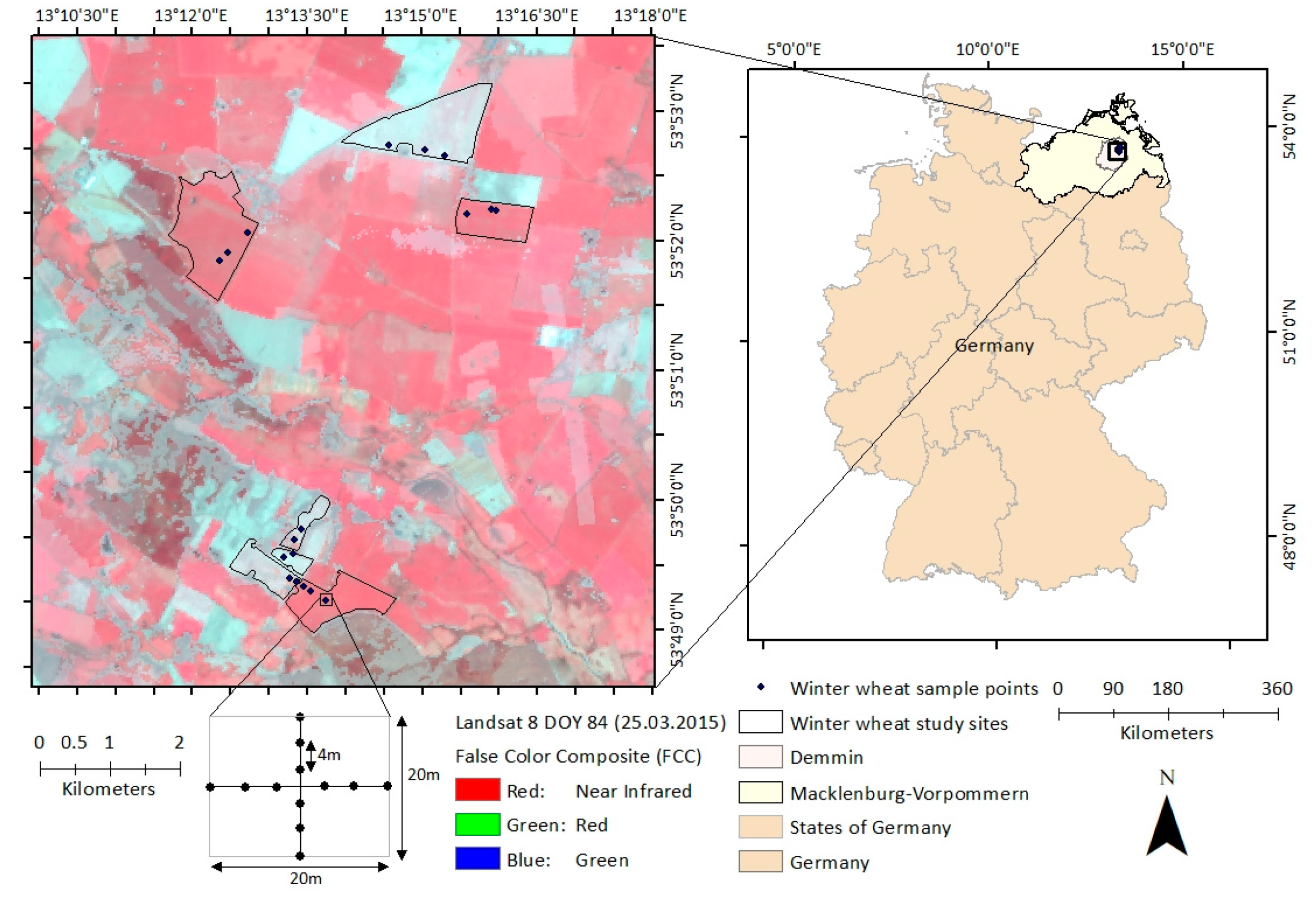
2.1. Study Area

The JECAM site DEMMIN is a part of the Northeast German Lowland Observatory that has been integrated into the Terrestrial Environmental Observatories (TERENO-NE) network from Helmholtz Association to fulfil the requirement of representing the landscape and climate conditions across Germany [51,52]. It is located near the city of Demmin in the federal state of Mecklenburg-West Pomerania in northeast Germany (Figure 1). Today’s landscape morphology of the study region is a result of the last glaciation; the topography of the northern part of the test site varies between 5 and 20 m, whereas the southern part is characterized by rolling hills several meters in height [53]. Grasslands cover about 25% of the area; these are mostly situated in the new flood plains; their soils are characterized by a high organic content, e.g., shallow peat soils [54]. Most of the region is intensively used for agricultural production [51]. The main crops grown are winter wheat, winter barley, winter rape, maize, potatoes, and sugar beet. Agricultural fields cover an area of approx. 30,000 ha and local farmers cultivate them. The soils are intermediate to high quality due to the rather fine-grained materials of the glacial till [51]. On average, the annual air temperature is about 8 ºC and the total precipitation reaches 600 mm [52,55].

2.2. Data Collection and Pre-processing

The climate data, biophysical data, and satellite data were obtained from multiple sources (

Table 1. Summary of the collected datasets for winter wheat crop modeling from start of season (SOS) to end of season (EOS) (dd.mm.yy). The climate parameters are maximum temperature (°C) (Tmax), minimum temperature (°C) (Tmin), dew point temperature (°C) (Tdew), relative humidity (%) (RH), clear sky surface photosynthetically active radiation (Wm-2) (PARCS), wind speed at 10 m (ms-1) (WIND), sunshine duration (s) (SUND), volumetric soil water layer 1 to 4 (m3) (SWVL1-4), top net solar radiation clear sky (Wm-2) (TSRC), and total precipitation (mm) (TP); the biophysical parameters are leaf area index (LAI) (m2 m-2), fraction of absorbed photosynthetic active radiation (FPAR), plant height (m) (PH), canopy cover (%) (CC) and biomass (g m-2); the satellite data are Landsat and Moderate Resolution Imaging Spectroradiometer (MODIS) MCD43A4.

Data	Product Name	Resolution		References
		Spatial	Temporal SOS–EOS
Climate data	Tmax, Tmin, Tdew, RH, PARCS, WIND, SUND, SWVL(1–4), TSRC, TP	~80 km	3 h 25.02.15–31.08.15	www.ecmwf.int
Biophysical data	FPAR, LAI, PH, CC, biomass	20 m	16 repeated measurements at dedicated BBCH *	www.jecam.org
Satellite data	Landsat 8	30 m	16 days 25.02.15–31.08.15	www.usgs.gov
	MODIS (MCD43A4)	500 m	1 day 25.02.15–31.08.15	www.lpdaac.usgs.gov

* Biologische Bundesanstalt, Bundessortenamt and Chemical Industry (BBCH) growth stages (initial, development, mid-, and late season).

). Firstly, the collected data were pre-processed according to the requirements of the study. After this step, the pre-processed information was integrated into the selected CGMs.

2.2.1. Climate Data

The climate data are available with a temporal resolution of 3 h for all elements mentioned above from the European Centre for Medium-Range Weather Forecasts’s (ECMWF) ERA-Interim for the period 25 Februay to 31 August in 2015. These three-hour based data are aggregated into daily means in order to fulfil the requirements of the CGMs. ECMWF provides global climate forecasts and historical climatic data at different spatial resolutions [56]. The spatial resolution of the climate data used in the study is approx. 80 km.

2.2.2. Biophysical Data

The biophysical parameters LAI, FPAR, plant height (PH), canopy cover (CC), and biomass are gathered on phenology based on the Biologische Bundesanstalt, Bundessortenamt and Chemical Industry (BBCH) characterization scale, such as in initial, development, mid-, and late season, and using various instruments, like a SunScan (FPAR), scanner (LAI), and height table (PH). An oven and a weighing machine were used to dry and weigh the collected wet biomass, respectively. In situ samples are acquired within seven winter wheat field sites on 16 days of the year (DOYs): 83, 84, 108, 109, 142, 144, 148, 149, 150, 151, 179, 180, 181, 182, 183, and 219. The sampling survey is designed into 18 sample points (also called as environmental sampling units (ESUs)) within 12 sub-plots per ESU, in the form of a rectangular cross with spatial extensions of 20 m by 20 m (Figure 1). A distance of 4 m separates each sub-plot. The measurements of the 12 subplots are averaged and assigned to the respective ESU.

The ESUs are far apart enough to not be displayed by the same Landsat pixel (30 m by 30 m). To measure the spatial auto-correlation between ESUs, the study conducts Moran’s I statistical test, which states a correlation of the values of a sample based on the measured locations. The test performs with the null hypothesis (H₀) that there is no spatial auto-correlation and the alternative hypothesis (H₁) that there is spatial auto-correlation [57,58,59]. The test is performed on samples considered at different time steps during the phenological cycle of winter wheat. For the present study, the results of Moran’s I were mostly negative, which indicates that the pattern of biomass sampling is dispersed with a non significant p-value (>0.05), which fails to reject the H₀.

2.2.3. Satellite Data

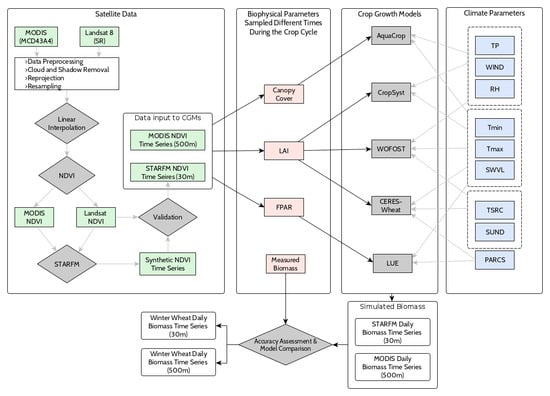
For the spatial–temporal analysis, the study makes use of Landsat 8 Surface Reflectance Code (LASRC) products and MODIS datasets. The LASRC Tier 1 has a spatial resolution of 30 m on a Universal Transverse Mercator (UTM) projection and provides seven spectral bands (coastal/aerosol, blue, green, red, near infrared (NIR), shortwave infrared (SWIR) 1, SWIR 2). The data is atmospherically corrected using LASRC. From the given quality assessment band “pixel_qa”, which is generated using the C function of mask (CFMask) algorithm, clouds and shadows are removed via the shadow and cloud masks. After preprocessing, the available cloud-free and shadow-free Landsat images were acquired in 2015 at the following DOYs respectively: 84 (25 March), 100 (10 April), 123 (03 May), 155 (04 June), 164 (13 June), 196 (15 July), and 219 (7 August). Additionally, the study uses MODIS MCD43A4 version 6 Nadir Bidirectional Reflectance Distribution Function (BRDF)-Adjusted Reflectance (NBAR) dataset that is produced daily using 16 days of Terra and Aqua MODIS data at 500 m spatial resolution. Both the cloud cover and the noise are removed from the quality index included in the product. The cloud gaps in the MODIS data are filled using the linear interpolation.

Eventually, the STARFM is used to fuse both the Landsat and MODIS datasets in order to generate a spatial temporal time series with higher spatial temporal resolution. Before applying the fusion algorithm, a single band of the NDVI from every time step has been generated from the reflectance bands of the Landsat and MODIS datasets. Prior to the data fusion, the MODIS daily NDVI dataset is reprojected and resampled to Landsat imagery using bilinear interpolation. The fused model is based on the principle that both the MODIS and Landsat products detect the same NDVI values, biased by a constant error due to their differences in data processing, acquisition time, bandwidth, and geolocation errors. The algorithm states that if a Landsat–MODIS image pair is available on the same DOY, this constant error can be calculated for each pixel in the image. After that, these errors can be applied to the available MODIS dataset of a prediction date to obtain a prediction image with the same spatial resolution of Landsat. According to [24], this is done in four different steps. Intially, the MODIS time series is reprojected and resampled to the available Landsat imagery. Next, a moving window is applied to the Landsat image to identify the similar neighboring pixels. After that, the weight W_I,j,k is assigned to each similar neighbor; lastly, the NDVI of the central pixel is calculated [24,30]. After obtaining the STARFM time series, the study validates the fused product by dropping a single available Landsat NDVI image during the fusion process and comparing both the real (dropped Landsat NDVI) and fused (STARFM NDVI) images of the same time zone. The STARFM performs the fusion process using Equation (1):

$$\mathrm{L}\left({\mathrm{x}}_{\frac{\mathrm{w}}{2}}{,\mathrm{y}}_{\frac{\mathrm{w}}{2}}{,\mathrm{t}}_{\mathrm{o}}\right)={\displaystyle \sum }_{\mathrm{i}=1}^{\mathrm{w}}{\displaystyle \sum }_{\mathrm{j}=1}^{\mathrm{w}}{\displaystyle \sum }_{\mathrm{k}=1}^{\mathrm{n}}{\mathrm{W}}_{\mathrm{ijk}}\ast (\mathrm{M}\left({\mathrm{x}}_{\mathrm{i}}{,\mathrm{y}}_{\mathrm{j}}{,\mathrm{t}}_{\mathrm{o}}\right)+\mathrm{L}\left({\mathrm{x}}_{\mathrm{i}}{,\mathrm{y}}_{\mathrm{j}}{,\mathrm{t}}_{\mathrm{k}}\right)-\mathrm{M}\left({\mathrm{x}}_{\mathrm{i}}{,\mathrm{y}}_{\mathrm{j}}{,\mathrm{t}}_{\mathrm{k}}\right)),$$

(1)

where w is the size of the moving window, L (x_w/2, y_w/2, t_o) is the cental pixel of the moving window for the Landsat image prediction at time t_o, and x_w/2, y_w/2 is the central pixel within the moving window. The spatial weighting function W_I,j,k determines how much each neighboring pixel x_i, y_j in w contributes to the estimated reflectance of the central pixel. (x_i, y_j, t_o) is the MODIS reflectance at the window location (x_i, y_j) observed at t_o, while L(x_i, y_j, t_k) and M(x_i, y_j, t_k) are the corresponding Landsat and MODIS pixel values observed at the base date t_k [24]. The n counts for total number of input pairs of (x_i, y_j, t_k) and M(x_i, y_j, t_k), and supposedly each pair is acquired on the same date. The size of the moving window is taken as 1500 m by 1500 m, which is three times the size of the MODIS pixel (500 m) and 50 times that of the Landsat pixel (30 m) [24]. The windows minimize the effect of pixel outliers and are therefore used for predicting changes using the spatially and spectrally weighted mean difference of pixels within the window area [24,40].

2.3. Methods

The study uses five different CGMs, namely, WOFOST, CERES-Wheat, AquaCrop, LUE, and CropSyst, to calculate crop biomass, including climate and biophysical variables as inputs (Figure 2) [44,45,46,47,48,49,50]. The selection of the models is based on their design, accuracy, and robustness, which have been proven in previous studies [60,61,62,63]. Because the CGMs lack the spatial information, fused RS time series and MODIS coarse resolution data are used to bridge this gap. Therefore, this study has modified the design of the models according to the input requirements. The developed approach uses the fused product to calculate the NDVI, the highly used indicator to monitor crop growth [17]. Prior input into CGMs, the STARFM NDVI pixel values that are less than 0 and more than 1 are removed from the time series. The ground-measured biophysical parameters (CC, LAI, and FPAR) and the NDVI generated from the STARFM and MODIS are used to derive the daily time series of their respective biophysical parameters, which is one of the input requirements for CGMs. For the remaining input parameters, the three-hour based climate variables are converted to a single day based on their daily mean values. Eventually, the model comparisons are made by validating the model-generated biomass with the measured biomass that is collected at repeated times of the year, based on both the STARFM and MODIS NDVI, individually (Section 2.2). The complete modeling design was adapted in the software R, with reference to the freely available design documentation of the abovementioned CGMs [64,65,66,67,68,69,70,71,72,73]. The parameters used to calibrate the abovementioned CGMs are taken from different related studies (

Table 2. Description of values used for calibrating the CGMs taken from the related literature.

Parameter	Description	Value	Units	Reference
ξ	Scattering coefficient	0.2	-	[44]
kdf	Diffusion coefficient	0.72	-	[74]
Am	Gross assimilation rate	4	g/m2	[75]
Ce	Conversion coefficient	0.0399	-	[76]
є	Light use efficiency	3	gC/MJ	[77]
CGC	Canopy growth	0.06	-	[78]
CDC	Canopy decline	0.05	-	[78]
WP	Water productivity	15–20	g/m2	[47]
Kbt	Crop potential transpiration	5	kPa	[79]

).

2.3.1. WOFOST

The WOFOST model describes the crop parameters, such as crop biomass and yield, by considering crop genetic properties and climatic parameters [44]. It states crop biomass as a function of solar radiation, temperature, and daily crop characteristics. It simulates the daily crop growth rate, which is the gross CO₂ assimilation rate that depends on the LAI and incoming radiation. The daily gross assimilation rate of the crop is calculated by the daily absorbed radiation and the photosynthetic characteristics of each leaf, and it further calculates the total carbohydrates (CH₂O) produced. Some fractions of the CH₂O produced are used to provide energy for respiration (maintenance respiration), and the remaining energy is converted into dry matter. The model calculates the growth rate as

∆G = C_e (A − R_m),

(2)

where ∆G is the growth rate (kg dry matter ha⁻¹ d⁻¹); A is the gross assimilation rate (kg CH₂O ha⁻¹ d⁻¹); R_m is the maintenance respiration rate (kg CH₂O ha⁻¹ d⁻¹); C_e is the conversion efficiency (kg dry matter kg⁻¹ CH₂O). Based on Monteith’s principle of light use efficiency, the calculation of total dry matter (kg dry matter ha⁻¹ yr⁻¹) in the WOFOST model is equivalent to the net primary production (NPP) (kg ha⁻¹ yr⁻¹) [48,80].

The complete process to calculate the per day growth of a crop’s biomass makes the WOFOST model complex in design. This study adopted the complete working methodology of this model from the WOFOST 6.0 documentation prepared by [81], which is also available online (www.wur.nl). A brief description of the WOFOST model is shown in Figure A1.

2.3.2. CERES-Wheat 2.0

The CERES-Wheat model is designed to simulate the effects of climatic parameters, soil, water stresses, and planting density on crop biomass and yield [82,83]. The study uses the CERES-Wheat 2.0 from the draft provided by Dr Joe T. Ritchie and Dr Doug Godwin. The model includes many climatic parameters, such as minimum and maximum temperature, solar radiation, soil moisture, and evapotranspiration. It estimates the biomass by generating the linear relationship between biomass production and intercepted radiation. This model is based on the principle of radiation use efficiency, demonstrating that the conversion efficiency of intercepted radiation to biomass is higher during periods of low radiation than those of high radiation [84]. The CERES-Wheat model calculates biomass as

Biomass = PCARB * Min(SWDF1, PRFT),

(3)

where PCARB is the potential biomass production (g m⁻² d⁻¹); SWDF1 is the soil water deficit (0;1); PRFT is the photosynthesis affected by temperature (0;1); Min is the minimum function which returns a minimum value. Similar to the WOFOST model, the biomass calculated by CERES-Wheat is equivalent to the NPP [48,80]. The detailed methodology of the CERES-Wheat model is shown in Figure A2.

2.3.3. AquaCrop 6.0–6.1

The AquaCrop model used in this study is proposed by [47], which describes the interactions between the plant and soil. It is used as a planning tool to understand the crop response to environmental changes. It subsequently estimates biomass from daily transpiration values. Moreover, it calculates the crop biomass using normalized water productivity (NCWP) based on the development of the crop canopy and crop transpiration. For this study, the crop transpiration and soil evaporation for the same model is calculated using the Penman–Monteith evapotranspiration equation given by [85]. The model calculates biomass as

Biomass = WP * ∑(T_r/ET_o),

(4)

where WP is the biomass water productivity (kg m⁻² d⁻¹); T_r is the transpiration (mm); ET_o is the reference evapotranspiration (mm). The step-wise methodology of the AquaCrop model is shown in Figure A3.

2.3.4. CropSyst

The CropSyst model simulates the effect of climate elements and soils on the total crop productivity [86]. The development of this model started in the early 1990s and simulates crop phenology, biomass, and crop yield. It calculates the daily biomass accumulation by determining potential biomass growth based on two components, potential transpiration and crop intercepted photosynthetically active radiation (PAR). The calculated potential growth is then corrected by water and temperature stress. According to [87], the model calculates the daily biomass production as

B_PT = (K_BT * T_p)/VPD,

(5)

where B_PT is the crop potential transpiration dependent biomass (g m⁻² d⁻¹), TP is the crop potential transpiration (g m⁻² d⁻¹), VPD is the mean atmospheric vapor pressure deficit (kPa), and Kbt is a biomass transpiration coefficient (kPa). The flow diagram of the CropSyst model is shown in Figure A4.

2.3.5. LUE

The working of the LUE model is based on the light use efficiency theory of [48,49]. However, few studies have integrated it with RS data. The study follows the same methodology to calculate the crop biomass calculated by using the technology of RS derived using a simple physiological paradigm modeled by [66,88]. The model is based on a semi-empiric approach and calculates the daily aboveground biomass as

Biomass = ∑ (PAR * fPAR) * є,

(6)

where PAR is photosynthetically active radiation (MJ m⁻² d⁻¹), fPAR is the fraction of PAR absorbed by the canopy, and є is the actual light-use efficiency (g C M J⁻¹). The total aboveground biomass calculated by the LUE model is equivalent to the NPP (kg ha⁻¹ yr⁻¹) [48,80]. The detailed step-wise procedure of the LUE model is shown in Figure A5.

2.4. Statistical Analysis

The STARFM NDVI data are validated with the pre-processed, cloud-free, and shadow-free Landsat images acquired during the study period. From the predicted NDVI (STARFM NDVI) and observed NDVI (Landsat NDVI), the determination coefficient (R²) (Equation (7)) and root mean square error (RMSE) (Equation (8) and Equation (9)) are calculated. Addtionally, after obtaining results from the CGMs, the modeled biomass of winter wheat obtained using the STARFM and MODIS NDVI is compared with the collected in situ biomass at different time steps during the study period. A linear regression model (LRM) is performed with an aim to establish a linear relationship between the measured (independent variable) and modeled biomass (dependent variable). The statistical parameters used to validate the accuracy of the CGMs are R², mean error (ME) (Equation (8)), and RMSE.

$${\mathrm{R}}^2=\frac{{({\displaystyle \sum }\left({\mathrm{P}}_i-\overline{P}\right)\left({\mathrm{O}}_i-\overline{O}\right))}^2}{{({\displaystyle \sum }\left(P_i-\overline{P}\right))}^2{({\displaystyle \sum }\left({\mathrm{O}}_i-\overline{O}\right))}^2},$$

(7)

$$\mathrm{ME}=\frac{1}{n}{\displaystyle \sum }_{i=1}^n{\left(O_i-P_i\right)}^2,$$

(8)

$$\mathrm{RMSE}=\sqrt{\mathrm{ME}},$$

(9)

where P_i is the predicted value, O_i is the observed value, Ō is the observed mean value, and n is the total number of observations.

R² is a statistical parameter which assesses how well measured values fit a model (i.e., it is a measure for the model quality) and RMSE is used to measure the quadratic differences between predicted and measured values (i.e., it is a measure for the model precision). In general, a lower RMSE value is better than a higher one. To check the significance of CGMs, the probability value (p-value) is calculated using an LRM with a H₀ that there is no correlation between the measured and predicted biomass, and an H₁ that the correlation exists. To perform this test, a significance level (also called alpha (α)) is set to 0.05. A p-value of less than 0.05 shows that a model is significant and it rejects the H₀ that there is no correlation.

2.5. Threshold Values of the Climate Parameters Used by CGMs

Many studies have explained growth model comparison, and in general, they show that less calibration causes more uncertainty for the output variable [89,90]. For a better accuracy, it is a crucial step to calibrate CGMs with their required climate parameters concerning the study site. The study uses a minimum lethal temperature value of −2 °C, which is used by [91] for winter wheat. One study [92] illustrated the minimum values of temperature for winter wheat at a grain growth stage as 12 °C. For VPD, this study follows [93], which has analyzed the atmospheric influences on leaf gas exchange on winter wheat with minimum and maximum values of 1.5 and 4.0 kPa, respectively. Ray et al. [94] considered four VPD values with a minimum of 1.1 kPa and a maximum of 3.6 kPa to measure its effect on the crop’s transpiration response to drying soil. Moreover, considering that the soil type of the Demmin region is loamy sand, the optimal soil parameter values of water content at field capacity, water content at the wilting point, maximum root depth (Zr), and the average fraction of total available water (TAW) (p) are 0.15 m³m⁻³, 0.06 m³m⁻³, 1.5–1.8 m, and 0.55, respectively (

Table 3. Description of the thresholds for climate variables used to calculate climate stress indices. All parameters included in the table are taken from different climate-related studies of winter wheat. Moreover, the values of these parameters are pre-designed in the CGMs before their implementation.

Parameter	Description	Value	Units	Reference
Tmin min	Minimum of minimum temperature	−2	°C	[91]
Tmin max	Maximum of minimum temperature	12	°C	[92]
VPD min	Minimum vapor pressure deficit (VPD)	1.3–1.5	k Pa	[93,94]
VPD max	Maximum VPD	3.6–4	k Pa	[93,94]
Zr max	Maximum root depth (Zr)	1.5–1.8	m	[95]
p	Average fraction of total available water (TAW)	0.55	-	[95]

).

3. Results

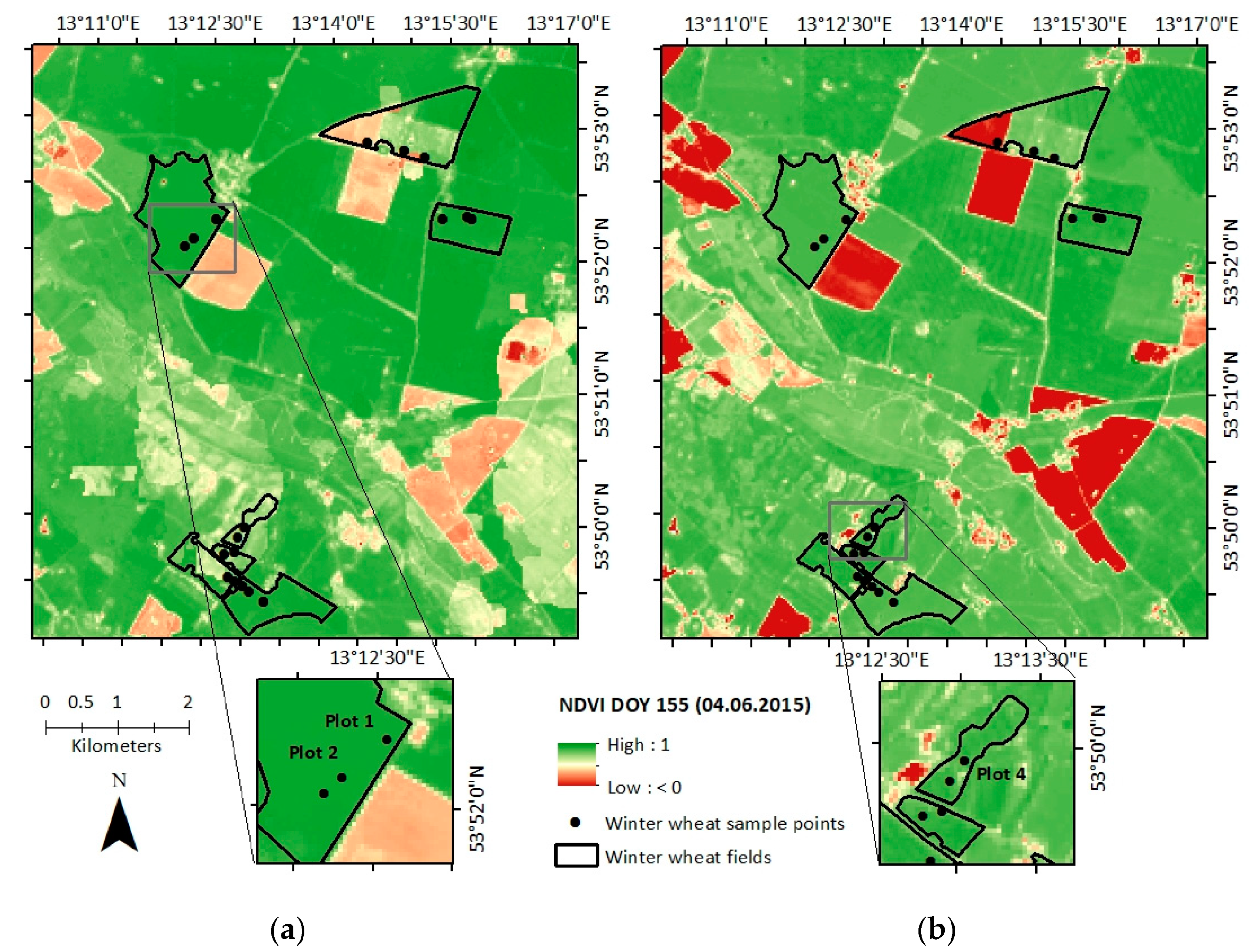
3.1. STARFM Data Fusion

The NDVI correlations between the Landsat and synthetic images for 2015 on available pre-processed Landsat dates are made to describe the quality, accuracy, and reliability of the STARFM product (Figure 3a–h). The identity line, or 1:1 line, in every plot compares the values of both the STARFM and Landsat NDVI data expected to be identical. However, an underestimation of pixels with lower NDVI values is observed in every plot. The R² values for the DOYs 100, 107, 155, and 164 show high correlations with values of 0.79, 0.84, 0.89, and 0.90, respectively. Besides, DOYs 107, 155, 164, and 180 have the lowest RMSEs of 0.08, 0.07, 0.06, and 0.07, in contrast to other dates, respectively. DOY 84 has the highest RMSE of 0.16 and the lowest R² of 0.45. The best correlation is observed for DOY 164 (13 June) with an R² of 0.90 and RMSE of 0.06. For the DOYs 196 and 219, the agreement of the reflectance values between the Landsat and the fused product is not as high. The R² value for both DOYs 196 and 203 is 0.65, with an RMSE of approx. 0.11. The highest values of RMSE are obtained for DOYs 84, 91, and 123 with the values 0.16, 0.17, and 0.10, respectively. Moreover, the lowest values of R² are obtained for the DOY 91, with a value of 0.40. When considering these numbers, it is necessary to note that they indicate the lowest quality of the fused product, as all real existing Landsat time series could be used to create the synthetic time series.

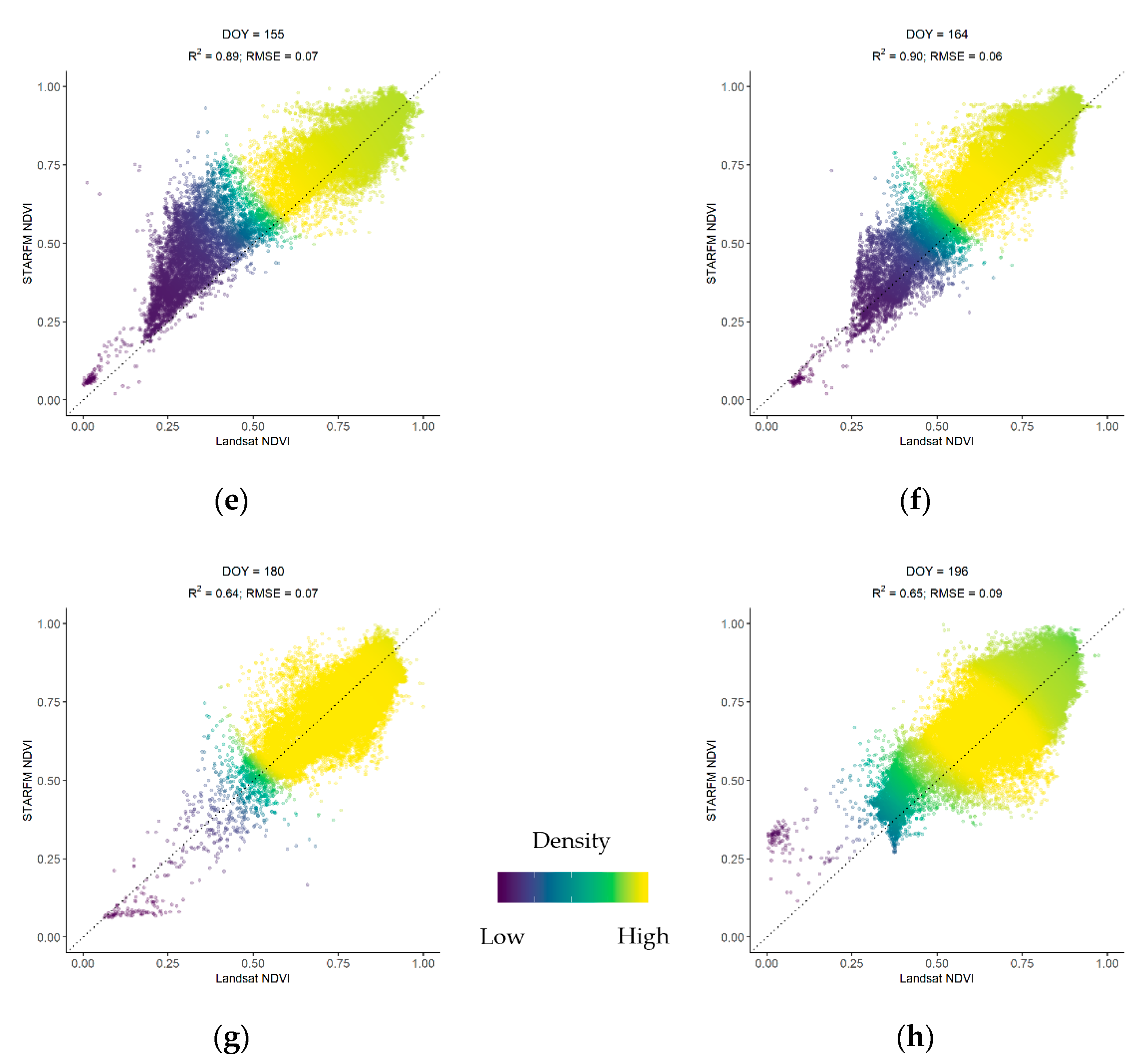
3.2. Fusion- and Landsat-Generated NDVI Comparison

Figure 4 shows the NDVI images produced by Landsat (Figure 4a) and the STARFM (Figure 4b) at the same resolution of 30 m of seven winter wheat fields on DOY 155. On a few sample points, the NDVI generated from the STARFM shows a slight underestimation of the values as compared to the Landsat; however, an opposite trend has been observed on other plots. A more detailed comparison is displayed in the subset maps of Figure 4, comparing three plots: Plot 1, Plot 2, and Plot 4. Plot 1 and Plot 2 show that the Landsat NDVI image is slightly greener than the one of the STARFM (i.e., NDVI values are higher on average). On the other hand, Plot 4 shows higher values of the STARFM NDVI comapared to the Landsat NDVI values. A plot-wise comparison of the selected three plots during the phenological cycle of winter wheat is shown in Figure 5a–c, which indicates both a slight underestimation and an overestimation of the NDVI values generated by the STARFM precisely during the development stages of winter wheat. Also, an overestimation of the NDVI values is observed during the late stages of the crop. Moreover, a similar trend is seen in the bar plots in Figure 5d–f for the same three plots. Importantly, the overall pattern followed by both NDVIs is very similar, thus, proving a sufficiently high accuracy and reliability of the fused time series for vegetation monitoring (overall R² of 0.618 and RMSE of 0.10).

3.3. CGM Evaluation

3.3.1. Statistical Comparison of CGMs

With both the STARFM and MODIS NDVI inputs, the five models performed significantly (having a p-value < 0.05); this rejects the H₀ of the LRM that there is no correlation between the modeled and measured crop biomass (Figure 6). The R² obtained from the STARFM product has a higher accuracy as compared to the MODIS. Based on the R² of the STARFM, the models are descendingly ordered as AquaCrop, LUE, CERES-Wheat, CropSyst, and WOFOST, with R² values of 0.86, 0.83, 0.78, 0.78, and 0.77, respectively. The MODIS R² values are: LUE (0.68), AquaCrop (0.65) and CERES-Wheat (0.63), CropSyst (0.55), and WOFOST (0.53). In general, the predicted values for all five models follow a similar pattern, and none of the models can claim to outclass the others. However, the ME and RMSE values give a more complete picture of the model performances (i.e., their quality and precision). The ME from the MODIS is slightly lower than the STARFM; on the contrary, the RMSE of the STARFM is lower than the MODIS. The overall STARFM range of all five models for the crop biomass estimation is from 333.11 to 435.29 g/m² (ME) and from 511.35 to 698.58 g/m² (RMSE). The CERES-Wheat model has provided the lowest RMSE of 511.35 g/m² and an ME of 333.11 g/m². Using MODIS, both WOFOST and AquaCrop have overestimated the biomass values as compared to the STARFM. However, the opposite trend has been observed in the remaining models.

3.3.2. Plotwise Comparison of CGMs using the STARFM

In the following, the models’ results obtained for the selected 18 plots are compared on a daily basis. The line graphs are drawn in Figure 7a–e show the increasing trend of biomass by all the CGMs and the biomass measured. The LUE model has shown an overestimation in the biomass values as compared to the other models. Except for CropSyst, the other CGMs show the same trend on a daily basis. In the CropSyst model, all ESUs show a dense pattern; however, the opposite is seen in the CERES-Wheat model, where the ESUs show a high variation. The AquaCrop model obtains almost similar values to the measured biomass at the initial stages of crop growth. However, a considerable variation is seen in almost all the models during the late development and mid-stages. After DOY 175, a stable trend in the increment of crop biomass is seen in all the selected models.

3.3.3. Spatial Distribution of Simulated Biomass by the Best Fit Models

Figure 8 shows the spatial distribution of simulated crop biomass at 30 m spatial resolution by the two best performing models: AquaCrop (Figure 8a) and LUE (Figure 8b) on DOY 171 (20 June) (i.e., nearly at the start or middle of the flowering stage of winter wheat). The minimum and maximum winter wheat biomass values vary between 1212.30 and 1554.81 g/m² in both the AquaCrop and LUE models. These values are obtained considering the climate stress factors, such as temperature stress, VPD, and soil moisture stress. This study shows AquaCrop and LUE are the best fit models with an R² of 0.86 and 0.83, and RMSEs of 522 and 582 g/m², respectively. The subset figures in Figure 8 show that the LUE model slightly overestimates the biomass values as compared to the AquaCrop model.

4. Discussion

4.1. Quality Assessment of Data Fusion

The study investigates the capability of the STARFM [24] over the northeastern region of Germany to predict seasonal changes in modeled biomass during 2015. The study uses the strategy “index-then-blend” (IB), which generates the NDVI from both Landsat and MODIS images before they are blended for the data fusion [96]. On the contrary, many studies first blend the reflectance of the individual MODIS and Landsat data sets and then generate the NDVI using the “blend-then-index”(BI) approach [97,98]. To investigate which is the better approach, [96] has conducted a theoretical and experimental analysis that states if the predicted NDVI values are lower than the input Landsat values, IB performs better and vice versa. In the present study, a few plots predict higher NDVI values and the remaining plots predict lower; therefore both BI and IB errors are expected to be small [96]. Additionally, the IB approach has less computation cost than BI, as it blends only one band: the NDVI. Therefore, in the present study it was decided to perform the fusion analysis using the IB approach.

The data fusion results indicate that the STARFM can successfully fuse MODIS and Landsat imagery [30,99]. The low RMSE and high R² obtained through the STARFM are comparable to those obtained by other studies [24,42,100]. The higher correlations between the observed and predicted NDVI values indicate the suitability of the algorithm for vegetation monitoring. However, many studies have suggested more improvements in the respective fusion algorithm [25,37,40].

In this study, Landsat and MODIS imagery are fused to create the synthetic NDVI time series with a 30 m spatial and daily temporal resolution. Due to high cloud coverage, which is typical in the study region, only four complete (DOYs: 84, 100, 164, and 219) and five partial (DOYs: 107, 123, 155, 180, and 196) cloud-free Landsat scenes were obtained during the phenological cycle of winter wheat. Due to the few cloud-free images, many gaps have been generated between the available Landsat scenes. Therefore, the accuracy of the produced fusion product has been affected [25,30]. For example, the small nine-day gap between DOYs 155 and 164 improves the quality of the fused product for respective days, having an R² of 0.89 and an RMSE of 0.06. However, the large gap between the Landsat images on DOYs 180 and 219 lowered the quality of the fused product obtained on day 219 with 0.65 (R²) and 0.13 (RMSE).

Previous studies have used multi-sensor data fusion to derive the NDVI as a monitoring tool for vegetation health and dynamics, allowing easy comparisons based on a temporal and spatial basis [15,32,33,97]. Assessing the reliability of the fused time series, the study compares the NDVI time series obtained from the fusion algorithm with the respective cloud-free Landsat scenes. Studies comparing multi-sensor NDVI values at the development stage of any vegetation reported that both Landsat and MODIS NDVI values are comparable within very close ranges, although the MODIS NDVI appears to be slightly higher than the Landsat NDVI because of its coarse spatial resolution of 500 m [101,102,103]. Similarly, the fused NDVI time series shows slight changes when compared at different growth stages of winter wheat. For example, a few plots show a small overestimation during the development stages and a high underestimation during the later stages of winter wheat, when compared with the real Landsat scenes on respective dates, and vice versa. For the points that have shown the overestimation, the reason could be because at later stages in the crop phenological cycle, the plants are ripe and turn yellowish due to a lower chlorophyll content [104]. Additionally, the MODIS 500 m coarse resolution covers the heterogeneity of green vegetation classes, such as forests or grasslands, which causes more uncertainty in the fused time series at later stages of a crop than the development or growth stages. Another reason could be the smaller gap of cloud-free Landsat data used for the STARFM fusion algorithm during the development stages than at the later stages of the crop.

4.2. Description of Results Obtained from Different Models

This study compares five different CGMs: WOFOST, AquaCrop, CERES-Wheat, LUE, and CropSyst to estimate crop biomass by inputting the MODIS and STARFM NDVI products individually. After obtaining the biomass values from different models, the present research compares the predicted values with the in situ biomass measurements taken from the sample plots at the DEMMIN test site. The obtained biomass values are a cumulative sum of each day of the crop growth cycle. These CGMs mentioned above differ in their complexity and processing time, and they have different requirements regarding the input variables. Overall, both the AquaCrop and LUE models perform well in achieving the desired balance of simplicity, accuracy, and robustness by simulating biomass satisfactorily compared to the observed records. For MODIS and the STARFM, both prove to be more reliable and significant with high R² (>0.64, >0.82,), low RMSE (<650 g/m², <600 g/m²), and p-value < 0.05, respectively. The CropSyst model works similar to the AquaCrop mode with regards to simplicity and its requirements for input parameters. However, it produces the crop biomass with the highest RMSE of 699 g/m² (STARFM) and 783 g/m² (MODIS), and the lowest R² of 0.78 (STARFM) and 0.55 (MODIS).

The study proves that the CGMs results obtained using the STARFM NDVI are more precise, accurate, and reliable than the MODIS. Even though the aim of the study is to generate a high spatial temporal time series for monitoring winter wheat, the results obtained from MODIS are still significant and precise, especially for AquaCrop, LUE, and CERES-Wheat. Moreover, it was found that CGMs, which require more input parameters, are not only more complex, but also need more processing time to generate the output. For example, both WOFOST and CERES-Wheat need many input parameters, such as evapotranspiration, relative humidity, PAR, soil moisture, solar radiation, and sunshine hours to calculate crop biomass, while AquaCrop, CropSyst, and LUEare designed to consider only three input variables. Even though WOFOST has a complex design, the biomass generated is less accurate, based on R² (0.77) and RMSE (651 g/m²) values when compared with the remaining models using the STARFM NDVI time series. In turn, the reason behind the degradation in the performance of WOFOST is the huge requirements for input parameters. Besides, for this model, there were still some missing crop parameters, like nitrogen uptake, stage-wise crop root density, percolation, and infiltration, that have affected the output. Similar to WOFOST, the CERES-Wheat model is purely based on mathematical equations. Besides its complexity, the model generates the output with the lowest RMSE of 511 g/m² using the STARFM and second lowest of 614 g/m² using MODIS.

4.3. Importance of Climate Parameters’ Spatial Resolution and Threshold Values

This study explains the importance of climate parameters, like minimum temperature, soil moisture, and VPD, in improving the accuracy of biomass estimation. As the present study is designed to implement CGMs at a global scale, the use of climate parameters from ECMWF is taken into consideration. However, the coarse spatial resolution of climate variables causes uncertainties in the model outputs. On the other hand, the DEMMIN test site has its own measuring stations that currently provide data, such as wind direction, wind speed, air temperature, air humidity, amount of rain and rain intensity, short-wave and long-wave radiation and counter-radiation, soil temperature and soil moisture at various depths, and air pressureevery 15 min. Conceptually, this study will be elaborated and validated by inputting interpolated data from measuring stations to improve the regional level accuracy of CGMs in the future. Moreover, the selection of suitable field- and crop-specific thresholds for the climate parameters is of high importance, as plant growth and development is strongly affected by climate elements [105]. The study used the threshold values of different climate parameters to improve the accuracy of calculated biomass. Some studies, exemplarily [106], highlighted the importance of the threshold values of climate parameters in crop production. The inclusion of climate threshold values plays an important role to get the impact of climate change on crop growth. However, in many CGMs, the knowledge of crop response to weather conditions is incomplete [107]. Hence, this causes a reduction in the performances of the simulation models and this further causes unreliability in crop yield prediction [108].

5. Conclusions

This study compares the performance of the five widely used CGMs: WOFOST, CERES-Wheat, AquaCrop, LUE, and CropSyst for the prediction of winter wheat biomass on the JECAM site DEMMIN, Germany. Because CGMs lack the spatial information to estimate the crop biomass at the field scale, the study bridges this gap by linking and comparing CGMs with the NDVI RS time series generated using the STARFM and MODIS. The capability of the STARFM is investigated by fusing both Landsat and MODIS imagery to create the synthetic NDVI time series, having a 30 m spatial and daily temporal resolution with an overall R² of 0.618 and RMSE of 0.10. Input satellite images with high cloud cover can deteriorate the quality of fused time series. The study makes use of 18 ESUs from seven winter wheat fields in 2015 to collect in situ biophysical parameters like LAI, FPAR, CC, and biomass with measurements repeated 16 times on a dedicated BBCH. The measured biomass is used to compare the performance of the CGMs based on the accuracy, simplicity, and reliability of the predicted biomass using the STARFM and MODIS NDVI time series. Overall, both the AquaCrop and LUE models perform well in achieving the desired balance, requiring only three input climate parameters and simulating biomass satisfactorily compared to the observed records, with high R² (>0.64, >0.82), low RMSE (<650 g/m², <600 g/m²), and significant p-values (<0.05) using MODIS and the STARFM, respectively. For the STARFM, the R² values obtained from the models are descendingly ordered as AquaCrop, LUE, CERES-Wheat, CropSyst, and WOFOST, with R² values of 0.86, 0.83, 0.78, 0.78, and 0.77, respectively. The study concludes that the CGM results obtained using the STARFM NDVI are more precise, accurate, and reliable than the MODIS.

Additionally, the study shows that the models requiring fewer input parameters (AquaCrop and LUE) to simulate crop biomass are highly applicable and significant. Meanwhile, they are easier to implement than the models WOFOST and CERES-Wheat, which need more input parameters, at least for winter wheat in moderate climate zones, such as the DEMMIN test site. On the contrary, due to the unavailability of some important crop-related parameters, such as crop management practices, the amount of fertiliser used, soil information, and seed type, the performance of some of the models was lowered. The inclusion of these parameters could result in a better performance. Moreover, the coarse spatial resolution of climate parameters (~80 km) likely also negatively affected the results of the CGMs. Thus, the validation of the present study with regional climate parameters from measuring stations of the DEMMIN test site is recommended and targeted for future investigations. Additionally, the present approach can also be extended to the correlation of biomass with the soil organic carbon at the test site, in order to analyze its impact on the crop yields.

References

1. Wheeler, T.; von Braun, J. Climate Change Impacts on Global Food Security. Science 2013, 341, 508–513. [Google Scholar] [CrossRef]
2. Agriculture Organization of the United Nations. The Future of Food and Agriculture-Trends and Challenges; Agriculture Organization of the United Nations: Rome, Italy, 2017. [Google Scholar]
3. Tirado, M.C.; Clarke, R.; Jaykus, L.A.; McQuatters-Gollop, A.; Franke, J.M. Climate change and food safety: A review. Food Res. Int. 2010, 43, 1745–1765. [Google Scholar] [CrossRef]
4. Gomiero, T.; Pimentel, D.; Paoletti, M.G. Is There a Need for a More Sustainable Agriculture? Crit. Rev. Plant Sci. 2011, 30, 6–23. [Google Scholar] [CrossRef]
5. Weiss, M.; Jacob, F.; Duveiller, G. Remote sensing for agricultural applications: A meta-review. Remote Sens. Environ. 2020, 236, 111402. [Google Scholar] [CrossRef]
6. Areal, F.J.; Jones, P.J.; Mortimer, S.R.; Wilson, P. Measuring sustainable intensification: Combining composite indicators and efficiency analysis to account for positive externalities in cereal production. Land Use Policy 2018, 75, 314–326. [Google Scholar] [CrossRef] [Green Version]
7. Di Falco, S.; Yesuf, M.; Kohlin, G.; Ringler, C. Estimating the impact of climate change on agriculture in low-income countries: Household level evidence from the Nile Basin, Ethiopia. Environ. Resour. Econ. 2012, 52, 457–478. [Google Scholar] [CrossRef]
8. Kasampalis, D.A.; Alexandridis, T.K.; Deva, C.; Challinor, A.; Moshou, D.; Zalidis, G. Contribution of remote sensing on crop models: A review. J. Imaging 2018, 4, 52. [Google Scholar] [CrossRef] [Green Version]
9. Murthy, V.R.K. Crop growth modeling and its applications in agricultural meteorology. Satell. Remote Sens. GIS Appl. Agric. Meteorol. 2004, 235–261. [Google Scholar]
10. Mirschel, W.; Schultz, A.; Wenkel, K.O.; Wieland, R.; Poluektov, R.A. Crop growth modelling on different spatial scales—A wide spectrum of approaches. Arch. Agron. Soil Sci. 2004, 50, 329–343. [Google Scholar] [CrossRef]
11. Clevers, J.G.P.W.; Vonder, O.W.; Jongschaap, R.E.E.; Desprats, J.F.; King, C.; Prevot, L.; Bruguier, N. Using SPOT data for calibrating a wheat growth model under mediterranean conditions. Agronomie 2002, 22, 687–694. [Google Scholar] [CrossRef]
12. Launay, M.; Guerif, M. Assimilating remote sensing data into a crop model to improve predictive performance for spatial applications. Agr. Ecosyst. Environ. 2005, 111, 321–339. [Google Scholar] [CrossRef]
13. Hansen, J.W.; Jones, J.W. Scaling-up crop models for climate variability applications. Agric. Syst. 2000, 65, 43–72. [Google Scholar] [CrossRef]
14. Belgiu, M.; Csillik, O. Sentinel-2 cropland mapping using pixel-based and object-based time-weighted dynamic time warping analysis. Remote Sens. Environ. 2018, 204, 509–523. [Google Scholar] [CrossRef]
15. Myneni, R.B.; Hall, F.G.; Sellers, P.J.; Marshak, A.L. The interpretation of spectral vegetation indexes. IEEE Trans. Geosci. Remote Sens. 1995, 33, 481–486. [Google Scholar] [CrossRef]
16. Doraiswamy, P.C.; Hatfield, J.L.; Jackson, T.J.; Akhmedov, B.; Prueger, J.; Stern, A. Crop condition and yield simulations using Landsat and MODIS. Remote Sens. Environ. 2004, 92, 548–559. [Google Scholar] [CrossRef]
17. Moriondo, M.; Maselli, F.; Bindi, M. A simple model of regional wheat yield based on NDVI data. Eur. J. Agron. 2007, 26, 266–274. [Google Scholar] [CrossRef]
18. Casa, R.; Varella, H.; Buis, S.; Guérif, M.; De Solan, B.; Baret, F. Forcing a wheat crop model with LAI data to access agronomic variables: Evaluation of the impact of model and LAI uncertainties and comparison with an empirical approach. Eur. J. Agron. 2012, 37, 1–10. [Google Scholar] [CrossRef]
19. Van Tricht, K.; Gobin, A.; Gilliams, S.; Piccard, I. Synergistic use of radar Sentinel-1 and optical Sentinel-2 imagery for crop mapping: A case study for Belgium. Remote Sens. 2018, 10, 1642. [Google Scholar] [CrossRef] [Green Version]
20. Drusch, M.; Del Bello, U.; Carlier, S.; Colin, O.; Fernandez, V.; Gascon, F.; Hoersch, B.; Isola, C.; Laberinti, P.; Martimort, P. Sentinel-2: ESA’s optical high-resolution mission for GMES operational services. Remote Sens. Environ. 2012, 120, 25–36. [Google Scholar] [CrossRef]
21. Middleton, E.M.; Ungar, S.G.; Mandl, D.J.; Ong, L.; Frye, S.W.; Campbell, P.E.; Landis, D.R.; Young, J.P.; Pollack, N.H. The earth observing one (EO-1) satellite mission: Over a decade in space. IEEE J. Sel. Top. Appl. Earth Obs. Remote Sens. 2013, 6, 243–256. [Google Scholar] [CrossRef]
22. Mulla, D.J. Precision Agriculture: Key Advances and Remaining Knowledge Gaps. Biosyst. Eng. 2013, 114, 358–371. [Google Scholar] [CrossRef]
23. Gao, F.; Anderson, M.C.; Zhang, X.; Yang, Z.; Alfieri, J.G.; Kustas, W.P.; Mueller, R.; Johnson, D.M.; Prueger, J.H. Toward mapping crop progress at field scales through fusion of Landsat and MODIS imagery. Remote Sens. Environ. 2017, 188, 9–25. [Google Scholar] [CrossRef] [Green Version]
24. Gao, F.; Masek, J.; Schwaller, M.; Hall, F. On the blending of the Landsat and MODIS surface reflectance: Predicting daily Landsat surface reflectance. IEEE Trans. Geosci. Remote Sens. 2006, 44, 2207–2218. [Google Scholar]
25. Roy, D.P.; Ju, J.; Lewis, P.; Schaaf, C.; Gao, F.; Hansen, M.; Lindquist, E. Multi-temporal MODIS–Landsat data fusion for relative radiometric normalization, gap filling, and prediction of Landsat data. Remote Sens. Environ. 2008, 112, 3112–3130. [Google Scholar] [CrossRef]
26. Dariane, A.B.; Khoramian, A.; Santi, E. Investigating spatiotemporal snow cover variability via cloud-free MODIS snow cover product in Central Alborz Region. Remote Sens. Environ. 2017, 202, 152–165. [Google Scholar] [CrossRef]
27. Parajka, J.; Blöschl, G. Spatio-temporal combination of MODIS images–potential for snow cover mapping. Water Resour. Res. 2008, 44, 1–13. [Google Scholar] [CrossRef]
28. Gafurov, A.; Bárdossy, A. Cloud removal methodology from MODIS snow cover product. Hydrol. Earth Syst. Sci. 2009, 13, 1361–1373. [Google Scholar] [CrossRef] [Green Version]
29. Dong, C.; Menzel, L. Improving the accuracy of MODIS 8-day snow products with in situ temperature and precipitation data. J. Hydrol. 2016, 534, 466–477. [Google Scholar] [CrossRef]
30. Gevaert, C.M.; García-Haro, F.J. A comparison of STARFM and an unmixing-based algorithm for Landsat and MODIS data fusion. Remote Sens. Environ. 2015, 156, 34–44. [Google Scholar] [CrossRef]
31. Lunetta, R.S.; Lyon, J.G.; Guindon, B.; Elvidge, C.D. North American landscape characterization dataset development and data fusion issues. Photogramm. Eng. Remote Sens. 1998, 64, 821–828. [Google Scholar]
32. Bhandari, S.; Phinn, S.; Gill, T. Preparing Landsat Image Time Series (LITS) for monitoring changes in vegetation phenology in Queensland, Australia. Remote Sens. 2012, 4, 1856–1886. [Google Scholar] [CrossRef] [Green Version]
33. Hwang, T.; Song, C.; Bolstad, P.V.; Band, L.E. Downscaling real-time vegetation dynamics by fusing multi-temporal MODIS and Landsat NDVI in topographically complex terrain. Remote Sens. Environ. 2011, 115, 2499–2512. [Google Scholar] [CrossRef]
34. Zhang, J. Multi-source remote sensing data fusion: Status and trends. Int. J. Image Data Fusion 2010, 1, 5–24. [Google Scholar] [CrossRef] [Green Version]
35. Belgiu, M.; Stein, A. Spatiotemporal image fusion in remote sensing. Remote Sens. 2019, 11, 818. [Google Scholar] [CrossRef] [Green Version]
36. Huang, B.; Song, H. Spatiotemporal reflectance fusion via sparse representation. IEEE Trans. Geosci. Remote Sens. 2012, 50, 3707–3716. [Google Scholar] [CrossRef]
37. Zhu, X.; Chen, J.; Gao, F.; Chen, X.; Masek, J.G. An enhanced spatial and temporal adaptive reflectance fusion model for complex heterogeneous regions. Remote Sens. Environ. 2010, 114, 2610–2623. [Google Scholar] [CrossRef]
38. Wu, M.; Niu, Z.; Wang, C.; Wu, C.; Wang, L. Use of MODIS and Landsat time series data to generate high-resolution temporal synthetic Landsat data using a spatial and temporal reflectance fusion model. J. Appl. Remote Sens. 2012, 6, 063507. [Google Scholar]
39. Zhu, X.; Helmer, E.H.; Gao, F.; Liu, D.; Chen, J.; Lefsky, M.A. A flexible spatiotemporal method for fusing satellite images with different resolutions. Remote Sens. Environ. 2016, 172, 165–177. [Google Scholar] [CrossRef]
40. Hilker, T.; Wulder, M.A.; Coops, N.C.; Linke, J.; McDermid, G.; Masek, J.G.; Gao, F.; White, J.C. A new data fusion model for high spatial-and temporal-resolution mapping of forest disturbance based on Landsat and MODIS. Remote Sens. Environ. 2009, 113, 1613–1627. [Google Scholar] [CrossRef]
41. Luo, Y.; Guan, K.; Peng, J. STAIR: A generic and fully-automated method to fuse multiple sources of optical satellite data to generate a high-resolution, daily and cloud-/gap-free surface reflectance product. Remote Sens. Environ. 2018, 214, 87–99. [Google Scholar] [CrossRef]
42. Emelyanova, I.V.; McVicar, T.R.; Van Niel, T.G.; Li, L.T.; Van Dijk, A.I.J.M. Assessing the accuracy of blending Landsat–MODIS surface reflectances in two landscapes with contrasting spatial and temporal dynamics: A framework for algorithm selection. Remote Sens. Environ. 2013, 133, 193–209. [Google Scholar] [CrossRef]
43. Zhu, X.; Cai, F.; Tian, J.; Williams, T.K.-A. Spatiotemporal fusion of multisource remote sensing data: Literature survey, taxonomy, principles, applications, and future directions. Remote Sens. 2018, 10, 527. [Google Scholar]
44. Van Diepen, C.A.V.; Wolf, J.; Van Keulen, H.; Rappoldt, C. WOFOST: A simulation model of crop production. Soil Use Manag. 1989, 5, 16–24. [Google Scholar] [CrossRef]
45. Ritchie, J.T.; Godwin, D.C.; Otter-Nacke, S. CERES-Wheat. A Simulation Model of Wheat Growth and Development; ARS US Department of Agriculture: Washington, DC, USA, 1985; Volume 252, pp. 159–175. [Google Scholar]
46. Raes, D.; Steduto, P.; Hsiao, T.C.; Fereres, E. AquaCrop—The FAO crop model to simulate yield response to water: II. Main algorithms and software description. Agron. J. 2009, 101, 438–447. [Google Scholar] [CrossRef] [Green Version]
47. Steduto, P.; Hsiao, T.C.; Raes, D.; Fereres, E. AquaCrop—The FAO crop model to simulate yield response to water: I. Concepts and underlying principles. Agron. J. 2009, 101, 426–437. [Google Scholar] [CrossRef] [Green Version]
48. Monteith, J.L. Solar radiation and productivity in tropical ecosystems. J. Appl. Ecol. 1972, 9, 747–766. [Google Scholar] [CrossRef] [Green Version]
49. Monteith, J.L. Climate and the efficiency of crop production in Britain. Philos. Trans. R. Soc. B Biol. Sci. 1977, 281, 277–294. [Google Scholar]
50. Stockle, C.O.; Martin, S.A.; Campbell, G.S. CropSyst, a cropping systems simulation model: Water/nitrogen budgets and crop yield. Agric. Syst. 1994, 46, 335–359. [Google Scholar] [CrossRef]
51. Zacharias, S.; Bogena, H.; Samaniego, L.; Mauder, M.; Fuß, R.; Pütz, T.; Frenzel, M.; Schwank, M.; Baessler, C.; Butterbach-Bahl, K. A network of terrestrial environmental observatories in Germany. Vadose Zone J. 2011, 10, 955–973. [Google Scholar] [CrossRef] [Green Version]
52. Borg, E.; Lippert, K.; Zabel, E.; Löpmeier, F.-J.; Fichtelmann, B.; Jahncke, D.; Maass, H. DEMMIN–Teststandort zur Kalibrierung und Validierung von Fernerkundungsmissionen. Rebenstorf RW (Ed.) 2009, 15, 401–419. [Google Scholar]
53. Dahms, T.; Seissiger, S.; Borg, E.; Vajen, H.; Fichtelmann, B.; Conrad, C. Important variables of a rapideye time series for modelling biophysical parameters of winter wheat. Photogramm. Fernerkund. Geoinf. 2016, 2016, 285–299. [Google Scholar] [CrossRef] [Green Version]
54. Castaldi, F.; Chabrillat, S.; Wesemael, V.B. Sampling strategies for soil property mapping using multispectral sentinel-2 and hyperspectral EnMAP satellite data. Remote Sens. 2019, 11, 309. [Google Scholar] [CrossRef] [Green Version]
55. Gerighausen, H.; Menz, G.; Kaufmann, H. Spatially explicit estimation of clay and organic carbon content in agricultural soils using multi-annual imaging spectroscopy data. Appl. Environ. Soil Sci. 2012, 2012, 1–23. [Google Scholar] [CrossRef]
56. Berrisford, P.; Kållberg, P.; Kobayashi, S.; Dee, D.; Uppala, S.; Simmons, A.J.; Poli, P.; Sato, H. Atmospheric conservation properties in ERA-Interim. Q. J. R. Meteorol. Soc. 2011, 137, 1381–1399. [Google Scholar] [CrossRef]
57. Gittleman, J.L.; Kot, M. Adaptation: Statistics and a null model for estimating phylogenetic effects. Syst. Zool. 1990, 39, 227–241. [Google Scholar] [CrossRef]
58. Paradis, E.; Claude, J.; Strimmer, K. APE: Analyses of phylogenetics and evolution in R language. Bioinformatics 2004, 20, 289–290. [Google Scholar] [CrossRef] [Green Version]
59. Cliff, A.D.; Ord, J.K. Spatial Processes: Models & Applications; Taylor & Francis: Oxfordshire, UK, 1981. [Google Scholar]
60. Confalonieri, R.; Bechini, L. A preliminary evaluation of the simulation model CropSyst for alfalfa. Eur. J. Agron. 2004, 21, 223–237. [Google Scholar] [CrossRef]
61. Bechini, L.; Bocchi, S.; Maggiore, T.; Confalonieri, R. Parameterization of a crop growth and development simulation model at sub-model components level. An example for winter wheat (Triticum aestivum L.). Environ. Model. Softw. 2006, 21, 1042–1054. [Google Scholar] [CrossRef]
62. Eitzinger, J.; Trnka, M.; Hösch, J.; Žalud, Z.; Dubrovský, M. Comparison of CERES, WOFOST and SWAP models in simulating soil water content during growing season under different soil conditions. Ecol. Model. 2004, 171, 223–246. [Google Scholar] [CrossRef]
63. Ma, G.; Huang, J.; Wu, W.; Fan, J.; Zou, J.; Wu, S. Assimilation of MODIS-LAI into the WOFOST model for forecasting regional winter wheat yield. Math. Comput. Model. 2013, 58, 634–643. [Google Scholar] [CrossRef]
64. Team, R.C. R: A Language and Environment for Statistical Computing; R Foundation for Statistical Computing, Vienna, Austria. 2013. Available online: https://www.gbif.org/tool/81287/r-a-language-and-environment-for-statistical-computing (accessed on 15 October 2017).
65. Wickham, H.; Francois, R.; Henry, L.; Müller, K. Dplyr: A grammar of data manipulation; R. Package. 2018. Available online: https://dplyr.tidyverse.org/ (accessed on 15 March 2019).
66. Dhillon, M.S.; Dahms, T.; Nill, L. Lue: R Package. 2018. Available online: https://cran.r-project.org/web/packages/lue/index.html (accessed on 12 March 2019).
67. Dragulescu, A.A.; Dragulescu, M.A.A.; Provide, R. Package ‘xlsx’. Cell 2020, 9, 1. [Google Scholar]
68. Bivand, R.; Keitt, T.; Rowlingson, B.; Pebesma, E.; Sumner, M.; Hijmans, R.; Rouault, E.; Bivand, M.R. Package ‘rgdal’. Bindings for the Geospatial Data Abstraction Library. Available online: https://cran/r-project/org/web/packages/rgdal/index/html (accessed on 15 October 2017).
69. Hijmans, R.J.; Van Etten, J.; Cheng, J.; Mattiuzzi, M.; Sumner, M.; Greenberg, J.A.; Lamigueiro, O.P.; Bevan, A.; Racine, E.B.; Shortridge, A. Package ‘Raster’. Geographic Data Analysis and Modelling. Available online: https://cran.r-project.org/web/packages/raster/index.html (accessed on 15 October 2017).
70. Wickham, H. ggplot2. Wiley Interdisciplinary Reviews: Computational Statistics. 2011, 3, pp. 180–185. Available online: https://ggplot2.tidyverse.org/ (accessed on 21 December 2017). [CrossRef]
71. Schwalb-Willmann, J. Getspatialdata: R Package. 2018. Available online: https://www.rdocumentation.org/packages/getSpatialData/versions/0.0.4 (accessed on 20 December 2018).
72. Dowle, M.; Srinivasan, A.; Gorecki, J.; Chirico, M.; Stetsenko, P.; Short, T.; Lianoglou, S.; Antonyan, E.; Bonsch, M.; Parsonage, H. Package ‘Data. Table’: Extension of ’Data. Frame; R. Package. 2019. Available online: https://www.rdocumentation.org/packages/getSpatialData/versions/0.0.4 (accessed on 20 December 2018).
73. Pierce, D. Ncdf4: Interface to Unidata Netcdf (Version 4 or Earlier) Format Data Files. 2012. Available online: http://CRAN,r-project,Org/package=ncdf4 (accessed on 15 October 2017).
74. Goudriaan, J. Crop Micrometeorology: A Simulation Study; Wageningen: Pudoc, Philippines, 1977. [Google Scholar]
75. Spitters, C.J.T.; Kramer, T.H. Differences between spring wheat cultivars in early growth. Euphytica 1986, 35, 273–292. [Google Scholar] [CrossRef] [Green Version]
76. Slattery, R.A.; Ort, D.R. Photosynthetic energy conversion efficiency: Setting a baseline for gauging future improvements in important food and biofuel crops. Plant Physiol. 2015, 168, 383–392. [Google Scholar] [CrossRef] [Green Version]
77. Djumaniyazova, Y.; Sommer, R.; Ibragimov, N.; Ruzimov, J.; Lamers, J.; Vlek, P. Simulating water use and N response of winter wheat in the irrigated floodplains of Northwest Uzbekistan. Field Crop. Res. 2010, 116, 239–251. [Google Scholar] [CrossRef]
78. Jin, X.; Li, Z.; Yang, G.; Yang, H.; Feng, H.; Xu, X.; Wang, J.; Li, X.; Luo, J. Winter wheat yield estimation based on multi-source medium resolution optical and radar imaging data and the AquaCrop model using the particle swarm optimization algorithm. ISPRS J. Photogramm. Remote Sens. 2017, 126, 24–37. [Google Scholar] [CrossRef]
79. Sinclair, T.R.; Tanner, C.B.; Bennett, J.M. Water-use efficiency in crop production. Bioscience 1984, 34, 36–40. [Google Scholar] [CrossRef]
80. Gitelson, A.A.; Peng, Y.; Masek, J.G.; Rundquist, D.C.; Verma, S.; Suyker, A.; Baker, J.M.; Hatfield, J.L.; Meyers, T. Remote estimation of crop gross primary production with Landsat data. Remote Sens. Environ. 2012, 121, 404–414. [Google Scholar] [CrossRef] [Green Version]
81. Supit, I. System description of the WOFOST 6.0 crop simulation model implemented in CGMS. Theory Algorithms 1994, 1, 146. [Google Scholar]
82. Ritchie, J.T.; Singh, U.; Godwin, D.; Hunt, L. A user’s guide to CERES-maize v2. 10. Int. Fertil. Dev. Cent. 1989, 2, 1–94. [Google Scholar]
83. Lobell, D.B.; Burke, M.B. On the use of statistical models to predict crop yield responses to climate change. Agric. For. Meteorol. 2010, 150, 1443–1452. [Google Scholar] [CrossRef]
84. Ritchie, J.T.; Singh, U.; Godwin, D.C.; Bowen, W.T. Cereal growth, development and yield. Understanding Options for Agricultural Production. Crop. Sci. 1998, 39, 79–98. [Google Scholar]
85. Zotarelli, L.; Dukes, M.D.; Romero, C.C.; Migliaccio, K.W.; Morgan, K.T. Step by Step Calculation of the Penman-Monteith Evapotranspiration (FAO-56 Method); The Institute of Food and Agricultural Sciences: Gainesville, FL, USA, 2010. [Google Scholar]
86. Stöckle, C.O.; Donatelli, M.; Nelson, R. CropSyst, a cropping systems simulation model. Eur. J. Agron. 2003, 18, 289–307. [Google Scholar] [CrossRef]
87. Tanner, C.B.; Sinclair, T.R. Efficient water use in crop production: Research or re-search? Limit. Effic. Water Use Crop. Prod. 1983, 1–27. [Google Scholar]
88. Shi, Z.; Ruecker, G.R.; Mueller, M.; Conrad, C.; Ibragimov, N.; Lamers, J.; Martius, C.; Strunz, G.; Dech, S.; Vlek, P.L.G. Modeling of cotton yields in the amu darya river floodplains of Uzbekistan integrating multitemporal remote sensing and minimum field data. Agron. J. 2007, 99, 1317–1326. [Google Scholar] [CrossRef]
89. Asseng, S.; Ewert, F.; Rosenzweig, C.; Jones, J.W.; Hatfield, J.L.; Ruane, A.C.; Boote, K.J.; Thorburn, P.J.; Rötter, R.P.; Cammarano, D. Uncertainty in simulating wheat yields under climate change. Nat. Clim. Chang. 2013, 3, 827–832. [Google Scholar] [CrossRef] [Green Version]
90. Rötter, R.P.; Palosuo, T.; Kersebaum, K.C.; Angulo, C.; Bindi, M.; Ewert, F.; Ferrise, R.; Hlavinka, P.; Moriondo, M.; Nendel, C. Simulation of spring barley yield in different climatic zones of Northern and Central Europe: A comparison of nine crop models. Field Crop. Res. 2012, 133, 23–36. [Google Scholar] [CrossRef]
91. Single, W.V. Frost injury and the physiology of the wheat plant. J. Aust. Inst. Agric. Sci. 1985, 5, 128–134. [Google Scholar]
92. Russell, G.; Wilson, G.W. An Agro-Pedo-Climatological Knowledge-Base of Wheat in Europe; Joint Reseach Centre: Brussels, Belgium, 1994. [Google Scholar]
93. Xue, Q.; Weiss, A.; Arkebauer, T.J.; Baenziger, P.S. Influence of soil water status and atmospheric vapor pressure deficit on leaf gas exchange in field-grown winter wheat. Environ. Exp. Bot. 2004, 51, 167–179. [Google Scholar] [CrossRef]
94. Ray, J.D.; Gesch, R.W.; Sinclair, T.R.; Allen, L.H. The effect of vapor pressure deficit on maize transpiration response to a drying soil. Plant Soil 2002, 239, 113–121. [Google Scholar] [CrossRef]
95. Allen, R.G.; Pereira, L.S.; Raes, D.; Smith, M. Crop evapotranspiration-Guidelines for computing crop water requirements-FAO Irrigation and drainage paper 56. Fao Rome 1998, 300, D05109. [Google Scholar]
96. Chen, X.; Liu, M.; Zhu, X.; Chen, J.; Zhong, Y.; Cao, X. “Blend-then-Index” or “Index-then-Blend”: A theoretical analysis for generating high-resolution NDVI time series by STARFM. Photogramm. Eng. Remote Sens. 2018, 84, 65–73. [Google Scholar] [CrossRef]
97. Walker, J.J.; De Beurs, K.M.; Wynne, R.H.; Gao, F. Evaluation of Landsat and MODIS data fusion products for analysis of dryland forest phenology. Remote Sens. Environ. 2012, 117, 381–393. [Google Scholar] [CrossRef]
98. Dong, T.; Liu, J.; Qian, B.; Zhao, T.; Jing, Q.; Geng, X.; Wang, J.; Huffman, T.; Shang, J. Estimating winter wheat biomass by assimilating leaf area index derived from fusion of Landsat-8 and MODIS data. Int. J. Appl. Earth Obs. Geoinf. 2016, 49, 63–74. [Google Scholar] [CrossRef]
99. Thorsten, D.; Christopher, C.; Babu, D.K.; Marco, S.; Erik, B. Derivation of Biophysical Parameters from Fused Remote Sensing Data. IEEE Xplore 2017, 374–4377. Available online: https://ieeexplore.ieee.org/stamp/stamp.jsp?arnumber=8127970 (accessed on 15 March 2018).
100. Chen, B.; Ge, Q.; Fu, D.; Yu, G.; Sun, X.; Wang, S.; Wang, H. A data-model fusion approach for upscaling gross ecosystem productivity to the landscape scale based on remote sensing and flux footprint modelling. Biogeosciences 2010, 7, 2943. [Google Scholar] [CrossRef] [Green Version]
101. Brown, M.E.; Pinzón, J.E.; Didan, K.; Morisette, J.T.; Tucker, C.J. Evaluation of the consistency of long-term NDVI time series derived from AVHRR, SPOT-vegetation, SeaWiFS, MODIS, and Landsat ETM+ sensors. IEEE Trans. Geosci. Remote Sens. 2006, 44, 1787–1793. [Google Scholar] [CrossRef]
102. Gao, X.; Huete, A.R.; Didan, K. Multisensor comparisons and validation of MODIS vegetation indices at the semiarid Jornada experimental range. IEEE Trans. Geosci. Remote Sens. 2003, 41, 2368–2381. [Google Scholar]
103. Huete, A.; Didan, K.; Miura, T.; Rodriguez, E.P.; Gao, X.; Ferreira, L.G. Overview of the radiometric and biophysical performance of the MODIS vegetation indices. Remote Sens. Environ. 2002, 83, 195–213. [Google Scholar] [CrossRef]
104. Yu, K.; Lenz-Wiedemann, V.; Chen, X.; Bareth, G. Estimating leaf chlorophyll of barley at different growth stages using spectral indices to reduce soil background and canopy structure effects. ISPRS J. Photogramm. Remote Sens. 2014, 97, 58–77. [Google Scholar] [CrossRef]
105. Porter, J.R.; Moot, D.J. Research Beyond the Means: Climatic Variability and Plant Growth, International Symposium on Applied Agrometeorology and Agroclimatology; Dalezios, N.R., Ed.; Office for Official Publication of the European Commission: Luxembourg, 1998; pp. 13–23. [Google Scholar]
106. Grace, J. Temperature as a determinant of plant productivity. Symp. Soc. Exp. Biol. 1988, 42, 91–107. [Google Scholar] [PubMed]
107. Porter, J.R.; Gawith, M. Temperatures and the growth and development of wheat: A review. Eur. J. Agron. 1999, 10, 23–36. [Google Scholar] [CrossRef]
108. Goudriaan, J. Predicting crop yields under global change. In Global Change and Terrestrial Ecosystems, International Geosphere-Biosphere Programme Book Series; Cambrige University Press: Cambridge, UK, 1996; Volume 2, pp. 260–274. [Google Scholar]
Figure 1. The location of the study region with an overview of 18 selected sample points and seven fields of winter wheat at the JECAM test site, DEMMIN, situated near the city of Demmin in the federal state of Mecklenburg-Vorpommern in northeast Germany. The background image represents the Landsat 8 imagery converted into a false color composite (FCC). A small subset shows the design of the sampling survey of one of the sample points, with 12 subplots in the form of a rectangular cross with a spatial extent of 20 m by 20 m. The distance between every subplot is four meters.
Remotesensing 12 01819 g001
Figure 2. Conceptual framework of the study that states the total input requirement of the crop growth models (CGMs), including various climate parameters, and biophysical parameters derived from the spatial and temporal reflectance adaptive reflectance fusion model (STARFM) and MODIS normalized difference vegetation index (NDVI) time series. The simulated biomass obtained from the CGMs is validated with the in situ biomass and CGMs are compared on the basis of simplicity, accuracy, and reliability using the STARFM and MODIS data sets. The end products are obtained as a winter wheat daily biomass time series of 30 m and 500 m spatial resolutions during the study period.
Remotesensing 12 01819 g002
Figure 3. Scatter plots of STARFM and Landsat NDVI images (ah) for the DOYs 84, 100, 107, 123, 155, 164, 180, and 196 during the study year, respectively. The values of statistical parameters, such as R2 and RMSE, are displayed at the top of each plot. Every plot contains a 1:1 line that is used to visualize the correlation of pixels between the STARFM and Landsat NDVI values. Colors in the scatter plots represent the density of points (low: blue and high: yellow) at different STARFM and Landsat NDVI values.
Remotesensing 12 01819 g003aRemotesensing 12 01819 g003b
Figure 4. Image-wise comparison of NDVIs obtained from Landsat and STARFM of a 30-m spatial resolution on DOY 155 (4 June); (a) NDVI image obtained from Landsat 8 (b) NDVI image obtained from the STARFM. Two subset maps at the bottom show a detailed spatial comparison of Plot 1, Plot 2, and Plot 4 on one of the winter wheat fields of the study region. The legend at the bottom center of the images shows the NDVI range from high: 1 (green) to low: <0 (red).
Remotesensing 12 01819 g004
Figure 5. Line plots showing the plot-wise comparison of NDVIs obtained from the Landsat and STARFM at Plot 1 (a), Plot 2 (b), and Plot 4 (c) during the phenological cycle of winter wheat in 2015. Similarly, the bar plots show the same comparison for (d) Plot 1, (e) Plot 2, and (f) Plot 4 during the study period. The yellow and green lines and bars represent the STARFM and Landsat NDVI values, respectively. The location of the plots is shown in Figure 4a.
Remotesensing 12 01819 g005
Figure 6. Scatter plots using an LRM using the STARFM and MODIS NDVI datasets as input variables to CGMs: (a) WOFOST, (b) CERES-Wheat, (c) AquaCrop, (d) CropSyst, and (e) LUE for the sample plots measured at different timesteps during the study period. The statistical parameters, R2, RMSE (g m−2), ME (g m−2) and p-value are displayed at the top of every scatter plot. The legend is displayed at the bottom center, where gray color represents MODIS and dark yellow represents the STARFM.
Remotesensing 12 01819 g006aRemotesensing 12 01819 g006b
Figure 7. Plot-wise comparison of simulated biomass obtained from CGMs: (a) WOFOST, (b) CERES-Wheat, (c) AquaCrop, (d) CropSyst, and (e) LUE for the 18 sample plots using the STARFM NDVI input during the study period. The line plots represent a unique color for every sample plot of the study region.
Remotesensing 12 01819 g007aRemotesensing 12 01819 g007b
Figure 8. Comparison of two best fit models: AquaCrop (a) and LUE (b) based on the spatial distribution of their simulated biomass obtained on DOY 171 using the STARFM NDVI input for winter wheat during the study period. The stretched legend at bottom left represents the maximum and minimum range of crop biomass from 1554.81 to 1212.3 g/m2. Two subset maps at the bottom of each image show the detailed spatial distribution of biomass for five sample plots distributed in two winter wheat fields of the study region.
Remotesensing 12 01819 g008