Dual-Frequency Airborne SAR for Large Scale Mapping of Tidal Flats

 , , , , , ,
  and
and
Abstract
:1. Introduction
2. Campaign over the North Sea
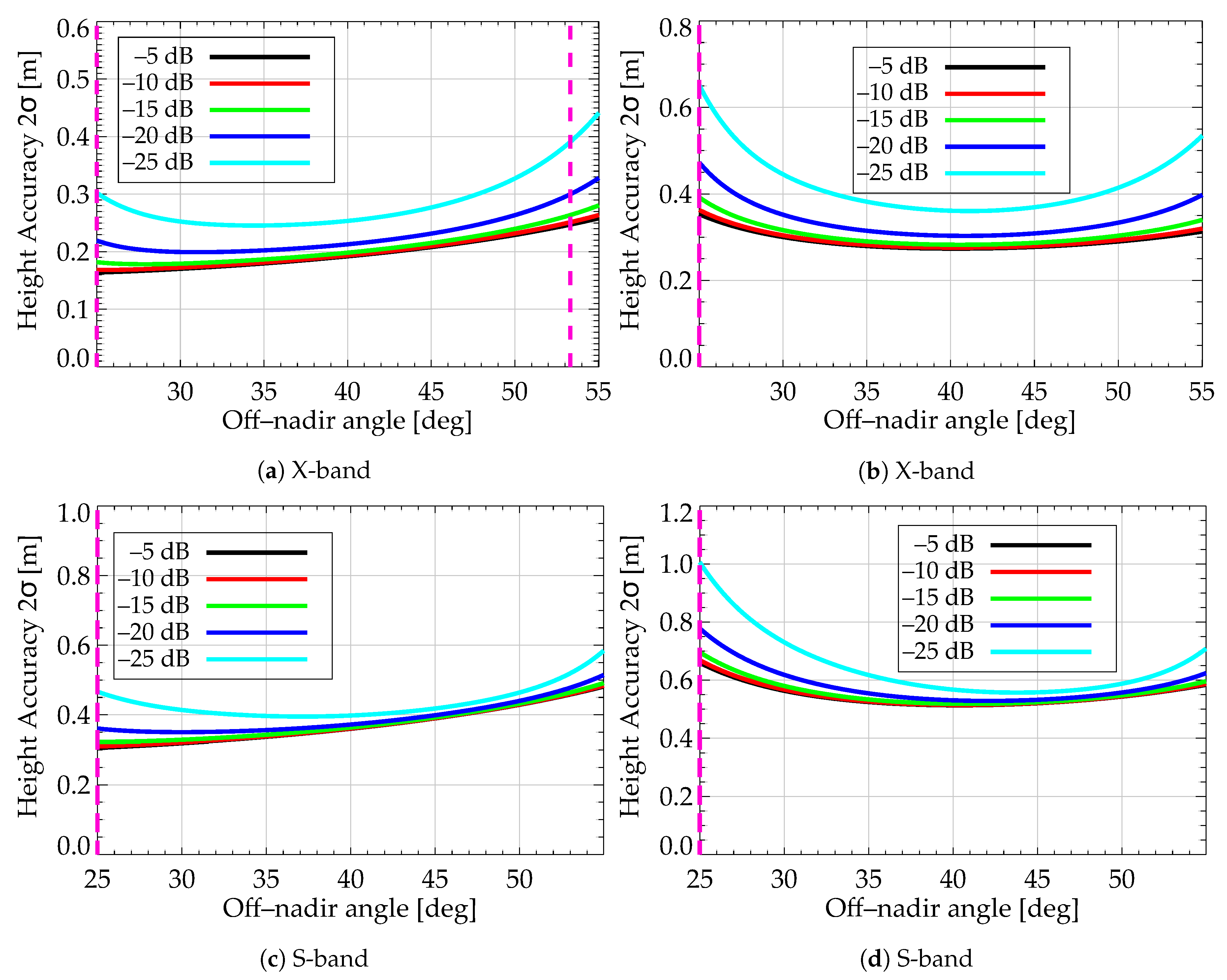
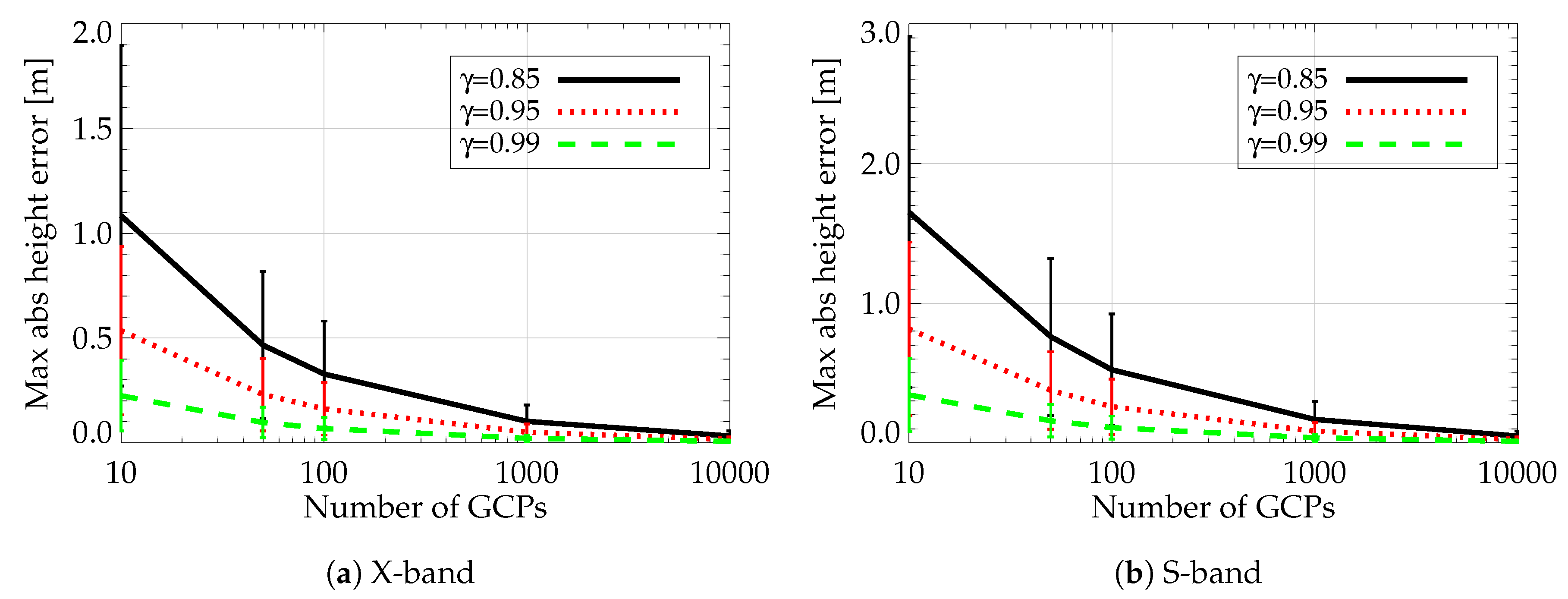
3. Baseline Selection and Expected Performance
4. Data Processing
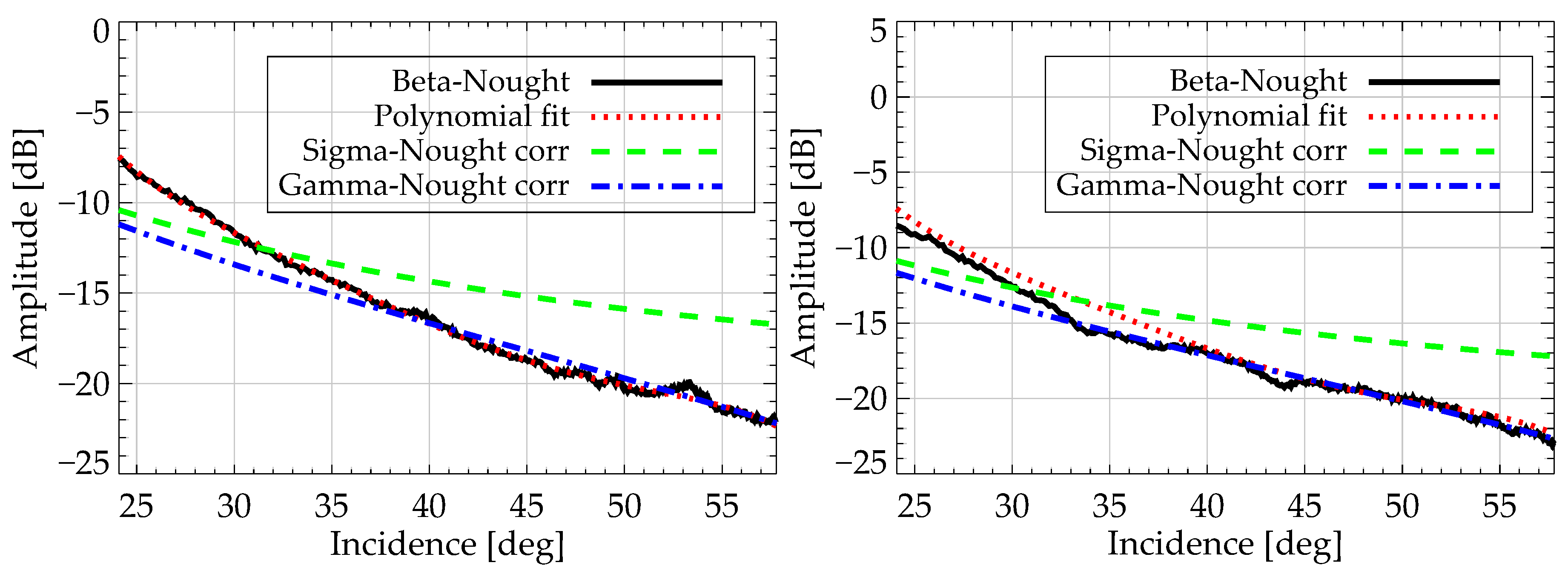
4.1. SAR Focusing and Calibration
4.2. DEM Generation
4.2.1. Generation of Interferometric Products
4.2.2. Dual-Frequency Phase Unwrapping
4.2.3. Baseline Calibration
4.2.4. Correction of Unwrapping Errors
4.2.5. Phase-to-Height Conversion
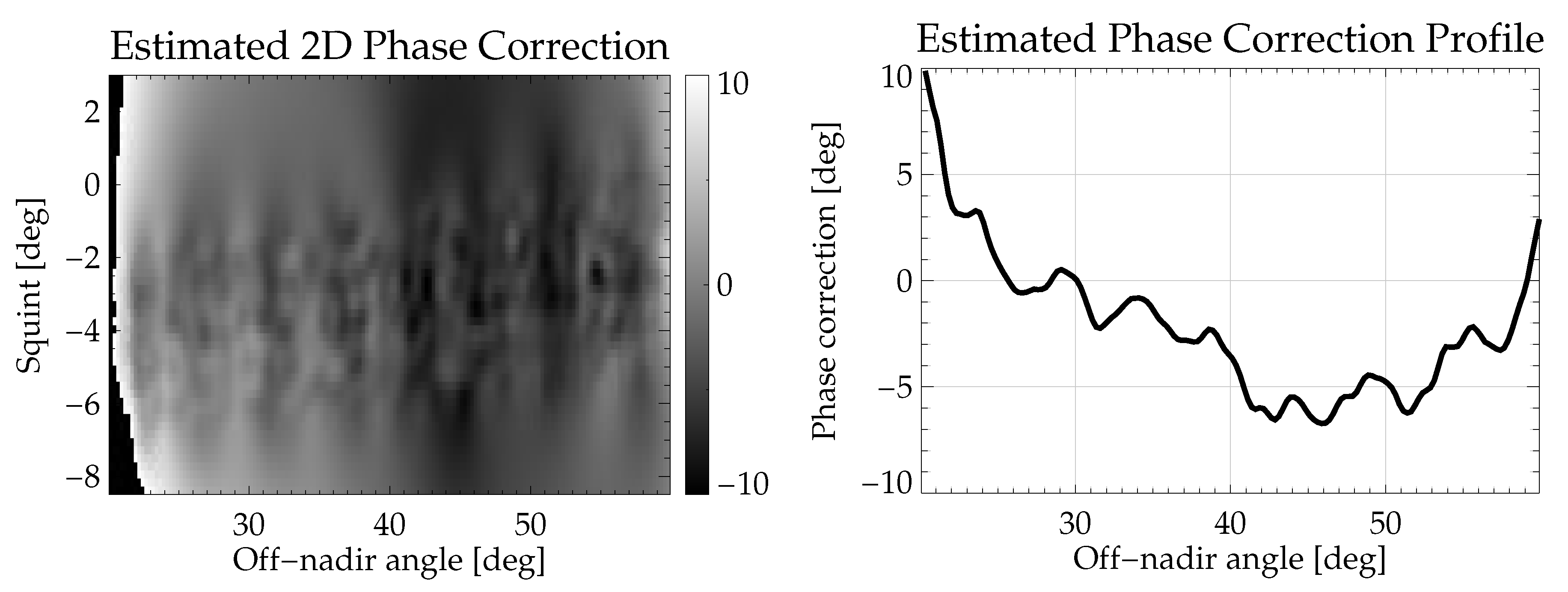
4.2.6. Residual Calibration
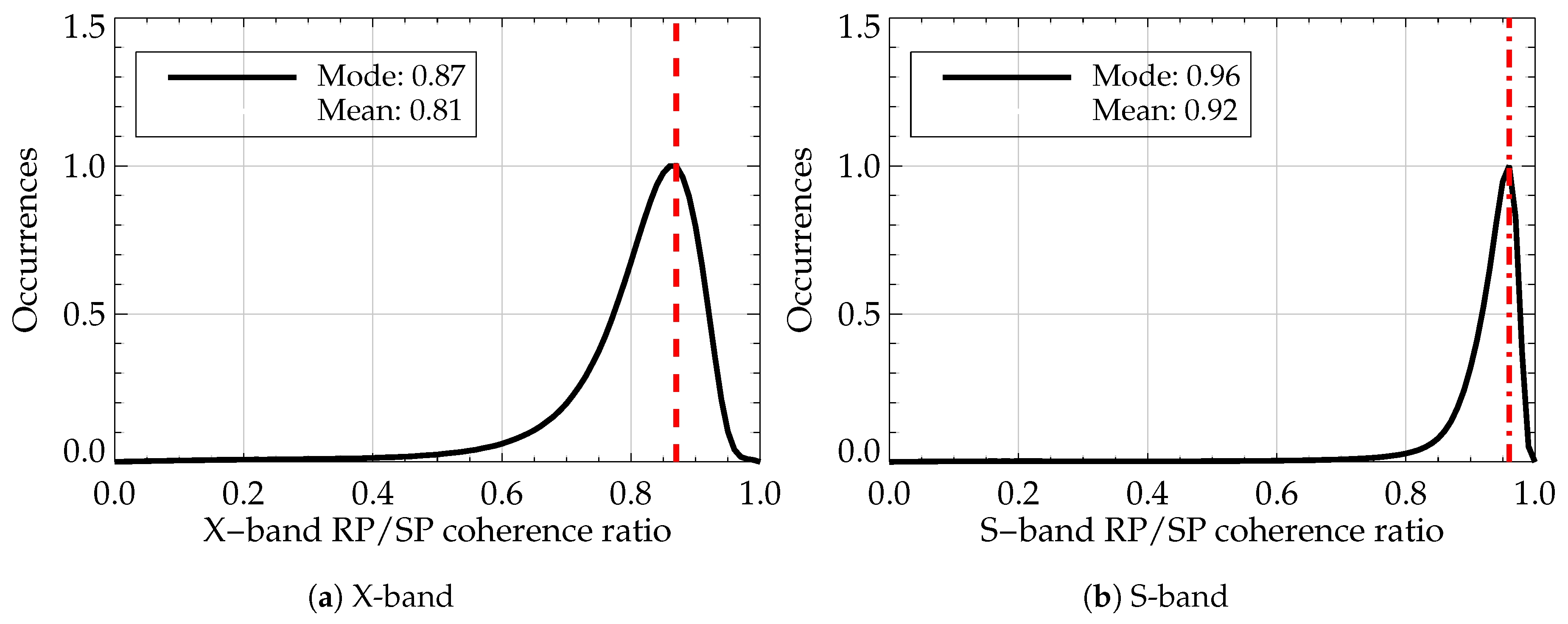
- considering the repeat-pass coherence to filter out flooded regions and vegetated areas, which are not consistent in the airborne SAR and reference DEMs.
- consider an outlier removal in order to account for differences in the topography, which might have happened in between acquisitions.
4.2.7. Generation of the Combined Repeat-Pass Height Map
4.2.8. Geocoding
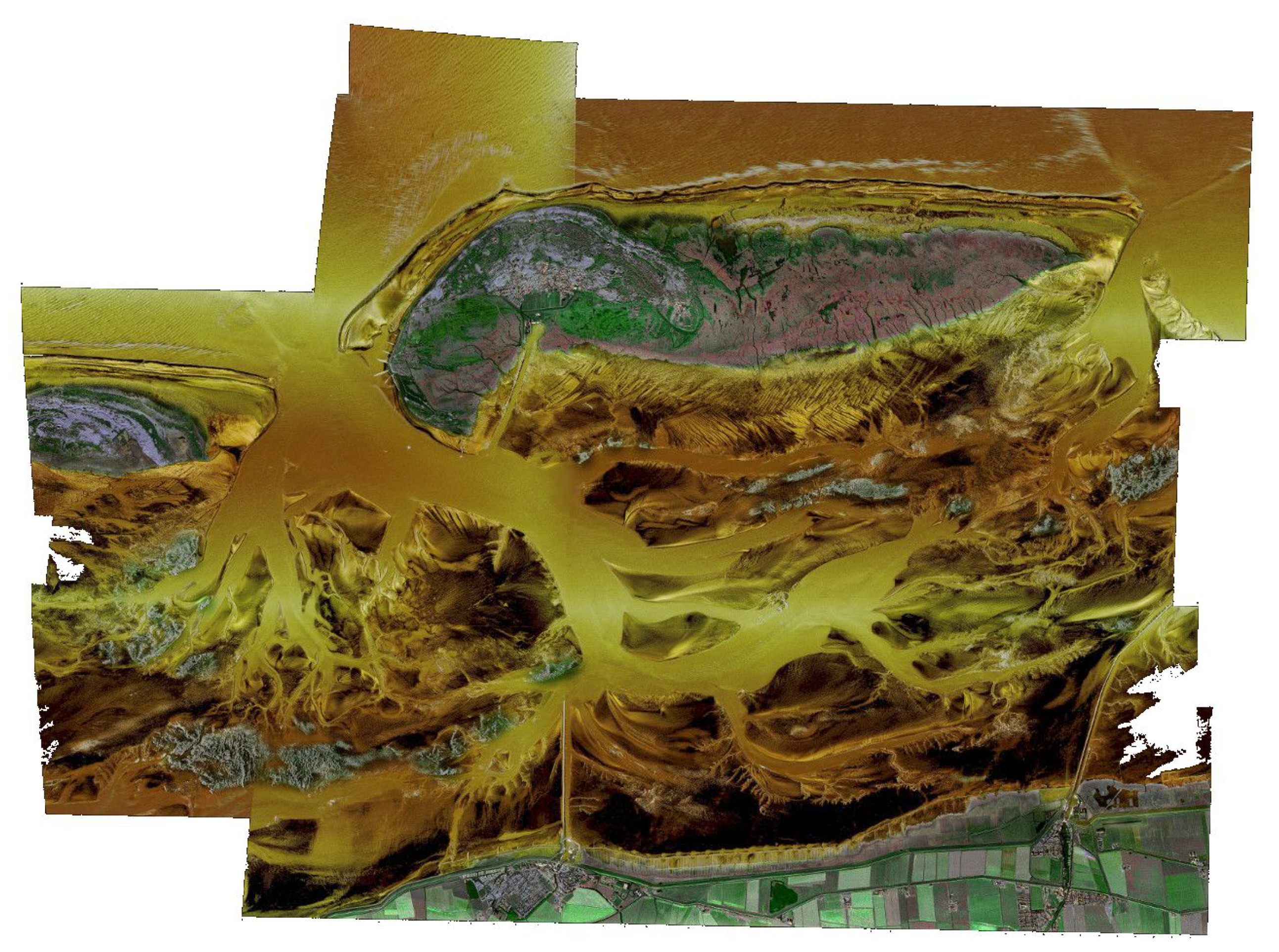
4.2.9. Mosaicking
4.3. Auxiliary Masks for Data Interpretation
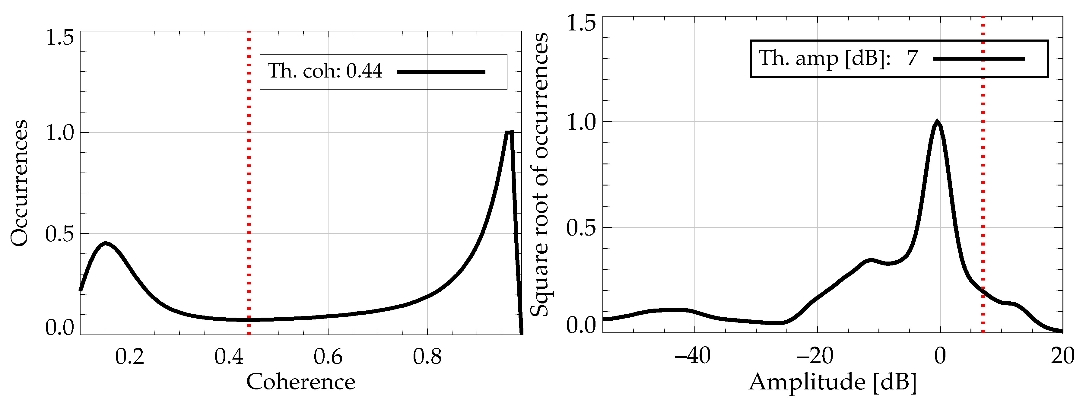
4.3.1. Interferometry Mask
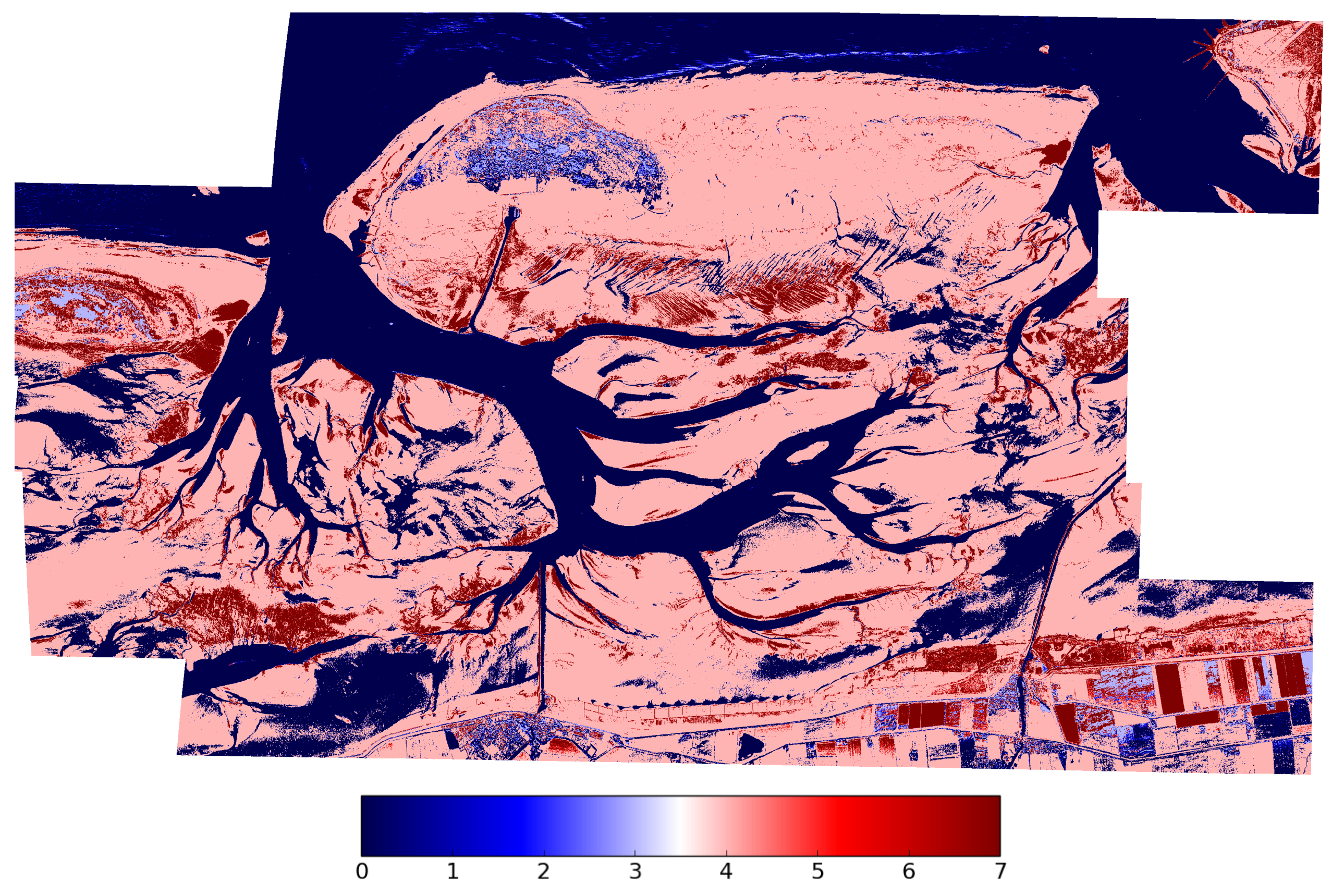
4.3.2. Polarimetry Mask
5. Results
6. Summary and Discussion
Author Contributions
Funding
Conflicts of Interest
References
- Wimmer, C.; Siegmund, R.; Schwabisch, M.; Moreira, J. Generation of high precision DEMs of the Wadden Sea with airborne interferometric SAR. IEEE Trans. Geosci. Remote Sens. 2000, 38, 2234–2245. [Google Scholar] [CrossRef]
- Hoja, D.; Lehner, S.; Niedermeier, A.; Romaneessen, E. DEM generation from ERS SAR shorelines compared to airborne crosstrack InSAR DEMs in the German Bight. In Proceedings of the IGARSS 2000 International Geoscience and Remote Sensing Symposium. Taking the Pulse of the Planet: The Role of Remote Sensing in Managing the Environment, Honolulu, HI, USA, 24–28 July 2000; Volume 5, pp. 1889–1891. [Google Scholar]
- Won, J.S.; Kim, S.W. ERS SAR Interferometry for Tidal Flat DEM. In Proceedings of the FRINGE 2003 Workshop, Frascati, Italy, 1–5 December 2003; Volume 550, p. 16. [Google Scholar]
- Hong, S.; Lee, C.; Won, J.; Kwoun, O.; Lu, Z. Spaceborne radar interferometry for coastal DEM construction. In Proceedings of the 2005 IEEE International Geoscience and Remote Sensing Symposium, IGARSS’05, Seoul, Korea, 25–29 July 2005; Volume 7, pp. 4806–4808. [Google Scholar]
- Park, J.W.; Choi, J.H.; Lee, Y.K.; Won, J.S. Intertidal DEM generation using satellite radar interferometry. Korean J. Remote Sens. 2012, 28, 121–128. [Google Scholar] [CrossRef]
- Wegmueller, U.; Santoro, M.; Werner, C.; Strozzi, T.; Wiesmann, A.; Lengert, W. DEM generation using ERS–ENVISAT interferometry. J. Appl. Geophys. 2009, 69, 51–58. [Google Scholar] [CrossRef]
- Kim, D.; Jung, J.; Choi, C.; Kang, K.; Kim, S.H.; Hwang, J. A long baseline airborne SAR interferometry for tidal flat mapping. In Proceedings of the 2016 URSI Asia-Pacific Radio Science Conference (URSI AP-RASC), Seoul, Korea, 21–25 August 2016; pp. 350–352. [Google Scholar]
- Kim, D. Measurement of Tidal Flat Topography using Long-Baseline InSAR. In Proceedings of the 2019 6th Asia-Pacific Conference on Synthetic Aperture Radar (APSAR), Xiamen, China, 26–29 November 2019; pp. 1–4. [Google Scholar]
- Lee, S.; Ryu, J. High-Accuracy Tidal Flat Digital Elevation Model Construction Using TanDEM-X Science Phase Data. IEEE J. Sel. Top. Appl. Earth Obs. Remote Sens. 2017, 10, 2713–2724. [Google Scholar] [CrossRef]
- Choi, C.; Kim, D. Optimum Baseline of a Single-Pass In-SAR System to Generate the Best DEM in Tidal Flats. IEEE J. Sel. Top. Appl. Earth Obs. Remote Sens. 2018, 11, 919–929. [Google Scholar] [CrossRef]
- Pinheiro, M.; Reigber, A.; Scheiber, R.; Prats-Iraola, P.; Moreira, A. Generation of Highly Accurate DEMs Over Flat Areas by Means of Dual-Frequency and Dual-Baseline Airborne SAR Interferometry. IEEE TGRS 2018, 56, 4361–4390. [Google Scholar] [CrossRef] [Green Version]
- Reigber, A.; Scheiber, R.; Jager, M.; Prats-Iraola, P.; Hajnsek, I.; Jagdhuber, T.; Papathanassiou, K.P.; Nannini, M.; Aguilera, E.; Baumgartner, S.; et al. Very-High-Resolution Airborne Synthetic Aperture Radar Imaging: Signal Processing and Applications. Proc. IEEE 2013, 101, 759–783. [Google Scholar] [CrossRef] [Green Version]
- Horn, R.; Nottensteiner, A.; Reigber, A.; Fischer, J.; Scheiber, R. F-SAR-DLR’s new multifrequency polarimetric airborne SAR. In Proceedings of the 2009 IEEE International Geoscience and Remote Sensing Symposium (IGARSS), Cape Town, South Africa, 12–17 July 2009; Volume 2, pp. 902–905. [Google Scholar]
- Bamler, R.; Hartl, P. Synthetic aperture radar interferometry. Inverse Probl. 1998, 14, R1–R54. [Google Scholar] [CrossRef]
- Lee, J.S.; Hoppel, K.; Mango, S.A.; Miller, A.R. Intensity and phase statistics of multilook polarimetric and interferometric SAR imagery. IEEE Trans. Geosci. Remote Sens. 1994, 32, 1017–1028. [Google Scholar]
- Pinheiro, M. Multi-Mode SAR Interferometry for High-Precision DEM Generation. Ph.D. Thesis, Karlsruher Institut für Technologie (KIT), Karlsruhe, Germany, 2016. [Google Scholar]
- Long, M. Radar Reflectivity of Land and Sea; Artech House: Boston, MA, USA; London, UK, 2001. [Google Scholar]
- Jäger, M.; Scheiber, R.; Reigber, A. External Calibration of Multi-Channel SAR Sensors Based on the Pulse-by-Pulse Analysis of Range Compressed Data. In Proceedings of the EUSAR 2018 12th European Conference on Synthetic Aperture Radar, Aachen, Germany, 4–7 June 2018. [Google Scholar]
- Jäger, M.; Scheiber, R.; Reigber, A. Robust, Model-Based External Calibration of Multi-Channel Airborne SAR Sensors Using Range Compressed Raw Data. Remote Sens. 2019, 11, 2674. [Google Scholar] [CrossRef] [Green Version]
- Pinheiro, M.; Reigber, A.; Moreira, A. Large-baseline InSAR for precise topographic mapping: A framework for TanDEM-X large-baseline data. Adv. Radio Sci. 2017, 15, 231–241. [Google Scholar] [CrossRef] [Green Version]
- Reigber, A. Range Dependent Spectral Filtering to Minimize the Baseline Decorrelation in Airborne SAR Interferometry. In Proceedings of the IEEE 1999 International Geoscience and Remote Sensing Symposium, Hamburg, Germany, 28 June–2 July 1999; Volume 3, pp. 1721–1723. [Google Scholar]
- Reigber, A.; Prats, P.; Mallorqui, J. Refined estimation of time-varying baseline errors in airborne SAR interferometry. Geosci. Remote Sens. Lett. IEEE 2006, 3, 145–149. [Google Scholar] [CrossRef]
- Wei, X.; Cumming, I. A region-growing algorithm for InSAR phase unwrapping. IEEE Trans. Geosci. Remote Sens. 1999, 37, 124–134. [Google Scholar] [CrossRef] [Green Version]
- Perna, S.; Esposito, C.; Berardino, P.; Pauciullo, A.; Wimmer, C.; Lanari, R. Phase Offset Calculation for Airborne InSAR DEM Generation Without Corner Reflectors. IEEE Trans. Geosci. Remote Sens. 2015, 53, 2713–2726. [Google Scholar] [CrossRef]
- Perna, S.; Esposito, C.; Berardino, P.; Lanari, R.; Pauciullo, A. A joint approach for phase offset estimation and residual motion error compensation in airborne SAR interferometry. In Proceedings of the 2014 IEEE Geoscience and Remote Sensing Symposium, Quebec City, QC, Canada, 13–18 July 2014; pp. 9–12. [Google Scholar]
- Gruber, A.; Wessel, B.; Martone, M.; Roth, A. The TanDEM-X DEM Mosaicking: Fusion of Multiple Acquisitions Using InSAR Quality Parameters. IEEE JSTARS 2016, 9, 1047–1057. [Google Scholar] [CrossRef]
- Knöpfle, W.; Strunz, G.; Roth, A. Mosaicking of Digital Elevation Models derived by SAR Interferometry. In The International Archives of Photogrammetry and Remote Sensing; Fritsch, D., Englich, M., Sester, S., Eds.; ISPRS Commission IV—GIS Between Visions and Applications: Stuttgart, Germany, 1998; Volume 32/4, pp. 306–313. [Google Scholar]
- Haklay, M.; Weber, P. Openstreetmap: User-generated street maps. IEEE Pervasive Comput. 2008, 7, 12–18. [Google Scholar] [CrossRef] [Green Version]
- Büttner, G.; Feranec, J.; Jaffrain, G.; Mari, L.; Maucha, G.; Soukup, T. The CORINE land cover 2000 project. EARSeL eProc. 2004, 3, 331–346. [Google Scholar]
- Bolz, T.; Schmitz, S.; Thiele, A.; Sörgel, U.; Hinz, S. Analysis of Airborne SAR and InSAR Data for Coastal Monitoring. Publ. Der Dtsch. Ges. Für Photogramm. Fernerkund. Und Geoinf. EV 2020, 29, 457–461. [Google Scholar]
- Schmitz, S.; Weinmann, M.; Weidner, U.; Hammer, H.; Thiele, A. Automatic Generation of Training Data for Land Use and Land Cover Classification by Fusing Heterogeneous Data Sets. Publ. Der Dtsch. Ges. Für Photogramm. Fernerkund. Und Geoinf. EV 2020, 29, 73–86. [Google Scholar]
- Raney, R.K.; Freeman, T.; Hawkins, R.W.; Bamler, R. A plea for radar brightness. In Proceedings of the IGARSS ’94-1994 IEEE International Geoscience and Remote Sensing Symposium, Pasadena, CA, USA, 8–12 August 1994; Volume 2, pp. 1090–1092. [Google Scholar]
- Valenzuela, G. Theories for the interaction of electromagnetic and oceanic waves — A review. Bound.-Layer Meteorol. 1978, 13, 61–85. [Google Scholar] [CrossRef]
- Cloude, S.R.; Pottier, E. An entropy based classification scheme for land applications of polarimetric SAR. IEEE Trans. Geosci. Remote Sens. 1997, 35, 68–78. [Google Scholar] [CrossRef]


| Parameter | X-Band | S-Band |
|---|---|---|
| Platform speed [m/s] | 90 | |
| Carrier frequency [GHz] | 9.78 | 3.25 |
| Transmitted bandwidth [MHz] | 300 | |
| Pulse repetition frequency (PRF) [Hz] | 3787 | 956 |
| Azimuth presumming factor | 8 | 2 |
| Range sampling frequency (RSF) [MHz] | 500 | |
| Pulse duration [μs] | 9 | |
| Azimuth resolution [m] | 0.5 | |
| Range resolution [m] | 0.5 | |
| Off-nadir angle [] | 25 to 55 | |
| Single-pass (SP) vertical baseline [m] | 1.5 | |
| SP horizontal baseline [m] | 0.4 | |
| Repeat-pass (RP) vertical baseline [m] | −40 | |
| RP horizontal baseline [m] | 0 | |
| Mean height above ground [m] | 2440 | |
| Bh | Bv | |
|---|---|---|
| Case 1 | −30 m | −30 m |
| Case 2 | −20 m | −20 m |
| Case 3 | −10 m | −30 m |
| Case 4 | 0 m | −40 m |
| Case 5 | 10 m | −40 m |
| Class | RP Coh | Master Amp | Slave Amp | Possible Interpretation |
|---|---|---|---|---|
| 0 | low | low | low | Water, shadow |
| 1 | low | low | high | Tidal channel, under water for master or slave pass |
| 2 | low | high | low | Tidal channel, under water for slave or master pass |
| 3 | low | high | high | Vegetation, crops and buildings |
| 4 | high | low | low | Dry tidal flat, bare soil, short vegetation |
| 5 | high | low | high | Unlikely |
| 6 | high | high | low | Unlikely |
| 7 | high | high | high | Bare soil, grass-land, mussel bed |
| Class | Entropy | Type of Reflection | Possible Class Interpretation |
|---|---|---|---|
| 0 | low | surface | Water, mudflat |
| 1 | medium | surface | Water, mudflat |
| 2 | high | surface | Unfeasible region |
| 3 | low | dipole | Vegetation with oriented structure |
| 4 | medium | vegetation | Short vegetation (grass) |
| 5 | high | vegetation | Tall vegetation |
| 6 | high | multiple | Tall vegetation (trees) |
| 7 | medium | multiple | Buildings |
| 8 | low | multiple | Buildings |
© 2020 by the authors. Licensee MDPI, Basel, Switzerland. This article is an open access article distributed under the terms and conditions of the Creative Commons Attribution (CC BY) license (http://creativecommons.org/licenses/by/4.0/).
Share and Cite
Pinheiro, M.; Amao-Oliva, J.; Scheiber, R.; Jaeger, M.; Horn, R.; Keller, M.; Fischer, J.; Reigber, A. Dual-Frequency Airborne SAR for Large Scale Mapping of Tidal Flats. Remote Sens. 2020, 12, 1827. https://doi.org/10.3390/rs12111827
Pinheiro M, Amao-Oliva J, Scheiber R, Jaeger M, Horn R, Keller M, Fischer J, Reigber A. Dual-Frequency Airborne SAR for Large Scale Mapping of Tidal Flats. Remote Sensing. 2020; 12(11):1827. https://doi.org/10.3390/rs12111827
Chicago/Turabian StylePinheiro, Muriel, Joel Amao-Oliva, Rolf Scheiber, Marc Jaeger, Ralf Horn, Martin Keller, Jens Fischer, and Andreas Reigber. 2020. "Dual-Frequency Airborne SAR for Large Scale Mapping of Tidal Flats" Remote Sensing 12, no. 11: 1827. https://doi.org/10.3390/rs12111827