Article

Evaluation of Six High-Spatial Resolution Clear-Sky Surface Upward Longwave Radiation Estimation Methods with MODIS

1
State Key Laboratory of Remote Sensing Science, Aerospace Information Research Institute, Chinese Academy of Sciences, Beijing 100101, China
2
University of Chinese Academy of Sciences, Beijing 100049, China
3
Environmental Futures Research Institute, School of Environment and Science, Griffith University, Nathan, QLD 4111, Australia
*
Author to whom correspondence should be addressed.
Remote Sens. 2020, 12(11), 1834; https://doi.org/10.3390/rs12111834
Submission received: 23 April 2020 / Revised: 2 June 2020 / Accepted: 2 June 2020 / Published: 5 June 2020

Abstract

:
Surface upward longwave radiation (SULR) is a critical component in the calculation of the Earth’s surface radiation budget. Multiple clear-sky SULR estimation methods have been developed for high-spatial resolution satellite observations. Here, we comprehensively evaluated six SULR estimation methods, including the temperature-emissivity physical methods with the input of the MYD11/MYD21 (TE-MYD11/TE-MYD21), the hybrid methods with top-of-atmosphere (TOA) linear/nonlinear/artificial neural network regressions (TOA-LIN/TOA-NLIN/TOA-ANN), and the hybrid method with bottom-of-atmosphere (BOA) linear regression (BOA-LIN). The recently released MYD21 product and the BOA-LIN—a newly developed method that considers the spatial heterogeneity of the atmosphere—is used initially to estimate SULR. In addition, the four hybrid methods were compared with simulated datasets. All the six methods were evaluated using the Moderate Resolution Imaging Spectroradiometer (MODIS) products and the Surface Radiation Budget Network (SURFRAD) in situ measurements. Simulation analysis shows that the BOA-LIN is the best one among four hybrid methods with accurate atmospheric profiles as input. Comparison of all the six methods shows that the TE-MYD21 performed the best, with a root mean square error (RMSE) and mean bias error (MBE) of 14.0 and −0.2 W/m2, respectively. The RMSE of BOA-LIN, TOA-NLIN, TOA-LIN, TOA-ANN, and TE-MYD11 are equal to 15.2, 16.1, 17.2, 21.2, and 18.5 W/m2, respectively. TE-MYD21 has a much better accuracy than the TE-MYD11 over barren surfaces (NDVI < 0.3) and a similar accuracy over non-barren surfaces (NDVI ≥ 0.3). BOA-LIN is more stable over varying water vapor conditions, compared to other hybrid methods. We conclude that this study provides a valuable reference for choosing the suitable estimation method in the SULR product generation.

Graphical Abstract

1. Introduction

The Earth’s surface radiation budget (SRB) is a driving factor in the exchange of energy between the atmosphere and oceans/land [1]. The SRB has a great influence on climate and land cover changes and is critical in ecological, hydrological and biogeochemical land surface processes [2]. The surface upward longwave radiation (SULR; the total surface upward radiative flux in the 4 to 100 μm spectral domain) is one of the four SRB components, and is the dominant component at night, high latitude, and during most times of the year in polar regions [3,4].
Satellite remote sensing plays an important role in regional and global terrestrial and atmospheric thermal condition studies [5,6]. Broadband satellite sensors which can directly measure the earth’s radiation up to 100 μm (e.g., Clouds and the Earth’s Radiant Energy System (CERES) [7,8]) are used for the generation of surface radiative flux products. Liang et al. [9] reviewed broadband satellite missions, sensors, products, and limitations. However, the spatial resolutions of such sensors are usually coarse (e.g., the spatial resolution of widely used CERES is 20km [10]). In the past two decades, narrow-band multispectral sensors with much higher spatial resolution (1–5 km), such as the Moderate Resolution Imaging Spectroradiometer (MODIS), have been used for SULR estimation. Several methods have been developed for instantaneous SULR estimation under clear-sky conditions from these fine spatial resolution satellite observations. In general, the SULR estimation methods proposed for multispectral sensors can be grouped into two categories.
The first category is temperature-emissivity physical methods [11,12], which calculates SULR using broadband land surface emissivity (LSE) estimates, land surface temperature (LST), and downward longwave radiation (DLR). Bisht et al. [11], Tang et al. [12], and Wang et al. [13] calculated the SULR using the MOD11 LST&LSE product. For the temperature-emissivity physical methods, the recently released MYD21 is a high-quality dataset available in the MODIS product collection 6. The MYD21 product is estimated using the Temperature/Emissivity Separation (TES) algorithm [14], whereas the MYD11 is based on the generalized split-window (SW) algorithm [15]. The TES algorithm used in the MYD21 simultaneously retrieves the LST and LSE from the MODIS thermal infrared bands 29, 31, and 32. However, the SW algorithm calculates the LST from bands 31 and 32 with the input of emissivity estimated by the classification-based emissivity method [16]. Therefore, the 5.6 km MYD11B1 LSEs estimated by a day/night algorithm (including bands 29, 31, and 32) are usually used to calculate the broadband emissivity instead of the 1 km MYD11_L2 LSEs of SW algorithm. As far as we know, the temperature-emissivity method with the LST and LSE inputs from the MYD21 data has not been evaluated in previous studies.
The other category is the hybrid framework [3,17,18,19], which directly estimates the SULR from satellite top-of-atmosphere (TOA) radiance through extensive radiative transfer simulation and linear statistical regression/nonlinear statistical regression/Artificial Neural Network (ANN) regression. The hybrid methods bypass the step of separating LST and LSE, but achieve the similar or in some cases higher accuracy than physical methods [13]. Wang et al. [13] first proposed the hybrid method and compared it with physical methods using MODIS data and Surface Radiation budget (SURFRAD) in situ SULR measurements. Jiao et al. [20] used the hybrid method to estimate SULR with MODIS and Visible Infrared Imaging Radiometer Suite (VIIRS) over the Tibetan Plateau. Cheng et al. [3] estimated global SULR using MODIS data with both the linear regression and neural network hybrid methods. Wang et al. [19] proposed a hybrid nonlinear model with split-window bands through introducing an equivalent temperature. In the previous hybrid SULR estimation methods, the atmospheric correction step is ignored and a relationship between SULR and TOA radiances is built directly. However, the relationship between SULR and bottom of atmosphere (BOA) radiances may be more stable because both of them are surface-related parameters. The surface outgoing radiance (Ioutgoing) at the BOA after atmospheric correction contains surface self-emitted and DLR information. The main difference between Ioutgoing and SULR is that SULR includes the sensor spectral response function (SRF) and hemispherical integrated solid angle (π), given that the thermal radiation is assumed to be isotropic [21]. Hu et al. [22] found that the narrow-band (7.5–13.5 μm with an almost Gaussian SRF) and wide-band (4–100 μm with unity SRF) Ioutgoing have a stable linear relationship with R2 > 0.999 for an airborne thermal infrared (TIR) sensor.
The purpose of this paper is to evaluate six methods for estimating instantaneous high-spatial resolution clear-sky SULR from MODIS satellite data using widely available SURFRAD in situ measurements as truth. These six methods include (1) the temperature-emissivity physical method from MYD11 (TE-MYD11), (2) the new temperature-emissivity physical method with MYD21 (TE-MYD21), (3) the hybrid method using TOA and linear regression (TOA-LIN), (4) the hybrid method using TOA and nonlinear regression (TOA-NLIN), (5) the hybrid method using TOA and ANN (TOA-ANN), and (6) the new hybrid method using BOA and linear regression (BOA-LIN). Both TE-MYD21 and BOA-LIN are newly developed SULR methods presented here. The data we used for the evaluation is presented in Section 2. The details of the two physical temperature-emissivity methods and four hybrid methods are introduced in Section 3. The evaluation results and discussions are demonstrated in Section 4. Finally, conclusions are given in Section 5.

2. Data and Processing

We conducted the evaluation with two datasets: a simulation dataset for the hybrid method comparison and a dataset containing two years of MODIS products and corresponding SURFRAD in situ measurements for the evaluation of all six methods. For the evaluation and coefficients calculation of hybrid methods, representative databases of typical atmospheric profiles and surface spectral emissivities are required to generate a simulation dataset of SULR and corresponding target variables (e.g., TOA radiances or BOA radiances in this study). The construction of the simulation dataset is introduced in Section 2.1. In the evaluation using MODIS and in situ measurements, the MODIS products (including TOA radiances, viewing zenith angle (VZA), geolocation, LST, narrow-band emissivity, and cloud information), atmospheric profiles (from ERA5), and in situ SULR measurement (from SURFRAD) are used. The data and corresponding processing steps are introduced in Section 2.2.

2.1. The Simulation Dataset for Hybrid Method

Representative databases of atmospheric profiles, LSTs and spectral LSEs are important to make the hybrid method fit real situations as much as possible. In this study we adopted the widely used Thermodynamic Initial Guess Retrieval (TIGR) database [23,24] database, which is composed of 2311 profiles measured from global atmospheric conditions. Based on the criterion that in all layers the relative humidity should be less than 90% [22], we selected 946 clear-sky profiles. The number of selected clear-sky atmospheric profiles for tropical, mid-latitude, and polar atmospheres is 236, 258, and 452, respectively. Their water vapor (wv) varies from 0.06 to 6.3 g/cm2 [25,26]. The LSTs were set with a (−10 K, 15 K) offset to the bottom temperature of the selected atmospheric profiles in a 5 K step. The LSEs (ε(λ)) were extracted from the MODIS UCSB (University of California, Santa Barbara) spectral library [27] which contains 158 emissivity spectra in the spectral range of 3.3 to 14.6 μm. To balance computation efficiency and surface representativeness, 35 typical emissivities were selected from different surface types, including three spectra for water, one spectrum for ice, one spectrum for snow, 13 spectra for soils and minerals, and 17 spectra for vegetation.
Postprocessing for the spectral LSEs is required because the spectral emissivity above 14 μm is not available in the MODIS UCSB library. Two extrapolation methods have been proposed to fill the gap between 14 μm and the upper wavelength boundary (i.e., 100 μm) for SULR estimation. Tang et al. [12] set the gap emissivity as unity. Wang et al. [28] developed an emissivity extrapolation method which is a linear combination of MODIS band 29, 31, and 32 emissivities (Equation (1)) and has been adopted in this paper.
{ ε 14 25 ¯ = 0.1828 ε 29 + 0.3867 ε 31 + 0.4395 ε 32 ε 25 100 ¯ = ε 14 25 ¯
where ε 29 , ε 31 , and ε 32 are the band-effective emissivity for MODIS band 29, 31, and 32, where ε 14 25 ¯ is the emissivity value in spectral range 14 to 25 μm calculated with narrow-band MODIS emissivity, and ε 25 100 ¯ is the emissivity value in spectral range 25 to 100 μm, which is set with the value of ε 14 25 ¯   .
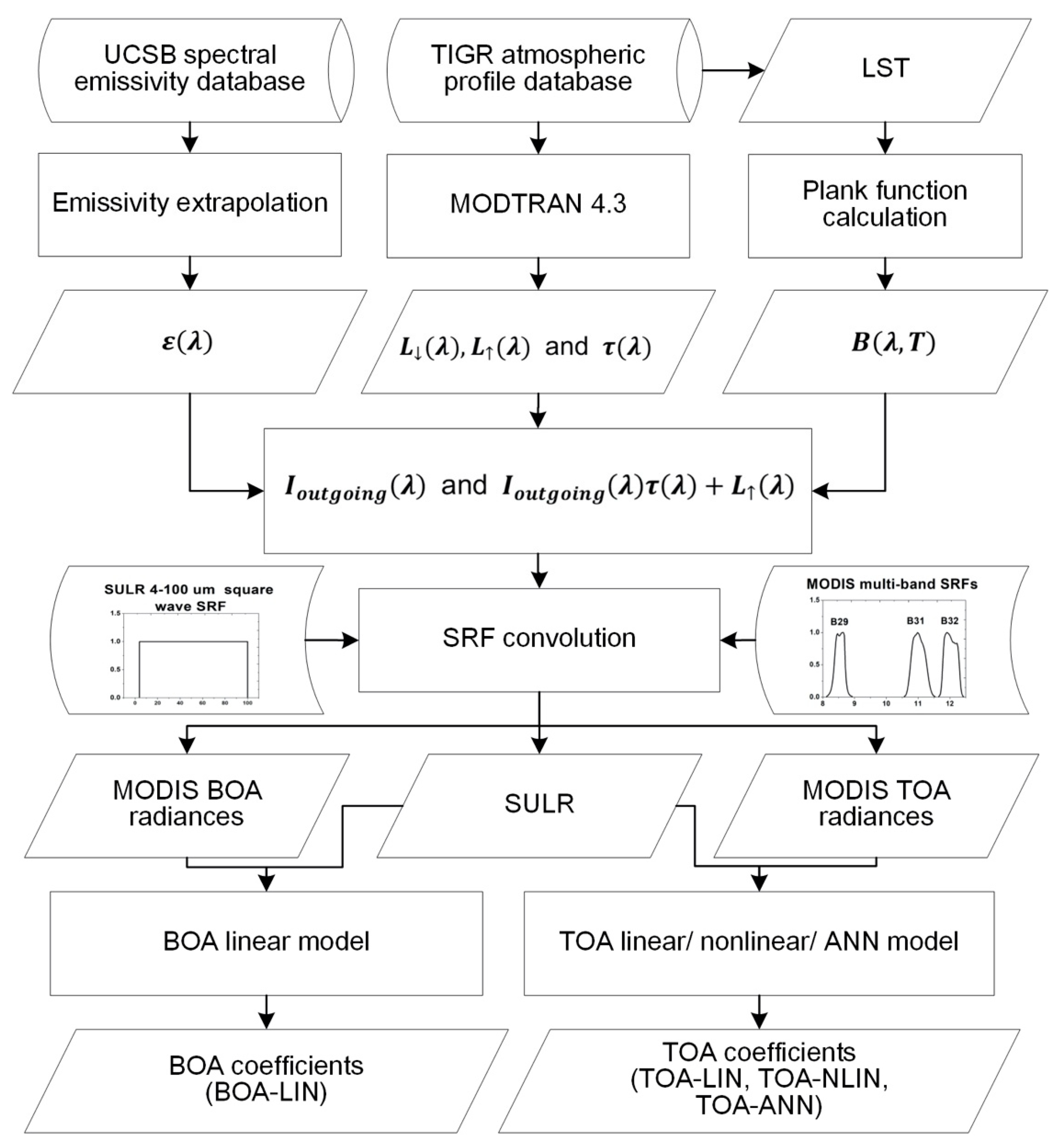
The MODerate resolution atmospheric TRANsmission (MODTRAN) model was selected to calculate the spectral atmospheric downwelling radiance (L(λ)), spectral atmospheric upwelling radiance (L(λ)), and spectral atmospheric transmittance (τ(λ)) with the inputs of 946 clear-sky TIGR atmospheric profile [29]. The surface spectral thermal emission (B(λ,T)) were obtained by the Plank function for the given wavelength (λ) and LST (T). The surface spectral outgoing radiances (Ioutgoing(λ)) include the self-emitted and reflected atmospheric downwelling radiance as shown in Equation (2). The SULR can be integrated with the Ioutgoing(λ) by Equation (3). The MODIS BOA radiances (LBOA,i) and TOA radiances (LTOA,i) of bands 29, 31, and 32 should consider the spectral response function (SRFi) using Equations (4) and (5) for BOA-LIN and TOA-LIN/NLIN/ANN, respectively.
I o u t g o i n g ( λ ) = ε ( λ ) B ( λ , T ) + ( 1 ε ( λ ) ) L ( λ )
  S U L R = π 4 100 I o u t g o i n g ( λ ) d λ  
  L B O A ,   i = λ 1 λ 2 I o u t g o i n g ( λ ) S R F i ( λ ) d λ λ 1 λ 2 S R F i d λ  
  L T O A ,   i = λ 1 λ 2 ( I o u t g o i n g ( λ ) τ ( λ ) + L ( λ ) ) S R F i ( λ ) d λ λ 1 λ 2 S R F i d λ  
In total, we carried out 198,660 (946 profiles × 6 temperatures × 35 emissivities) simulations. Here, one simulation includes the SULR value and the corresponding TOA/BOA radiances of MODIS bands 29, 31, and 32.

2.2. The Evaluation Datasets with MODIS, ERA5 and In Situ Measurements

The flowchart of data processing for the MODIS, ERA5, and in situ measurements is shown in Figure 1. First, the MODIS clear-sky pixels were screened with the MODIS cloud product. Then, the clear-sky LSTs, LSEs, and the in situ measured DLR in SURFRAD stations were used to drive the temperature-emissivity methods (TE-MYD21 and TE-MYD11) and the clear-sky TOA radiances, and the coefficients of TOA methods were used to drive the TOA hybrid methods (TOA-LIN, TOA-NLIN, and TOA-ANN). The data processing for the BOA-LIN method includes four steps: (1) Extracting the atmospheric profiles form ERA5 global reanalysis product based on geolocation (latitude and longitude) and the Shuttle Radar Topography Mission (SRTM) digital evaluation model (DEM) [30]; (2) calculating the atmospheric parameters (τ, L and L) using ERA5 atmospheric profiles; (3) performing the atmospheric correction from clear-sky TOA radiances to BOA radiances using the atmospheric parameters; (4) calculating the SULR using the BOA radiances with BOA coefficients. Finally, the six methods were evaluated using the SURFRAD SULR in situ measurements.

2.2.1. MODIS Datasets

The MODIS instruments onboard satellite Terra (Aqua) have been observing the Earth continuously since 1999 (2002). MOD21 product has not been produced beyond 2005 because it requires bands 29, 31, and 32 as inputs and the infrared bands 27–30 of Terra-MODIS have been negatively impacted by an optical crosstalk issue since 2005. Observations from 2017 to 2018 were considered here; therefore, only the MYD products generated from Aqua-MODIS are used. The Aqua-MODIS is a whisk-broom sensor with a cross track and along track swath of 2330 km x× 10 km. Its maximum VZA at the image edge is >60 degrees. The sensor has 36 spectral bands located in the 0.405 to 14.385 μm range, with spatial resolutions of 1000 m in the TIR bands. MODIS currently has 44 data products, which can be grouped into 5 classes: calibration, atmosphere, land, cryosphere and ocean. All these data can be found and downloaded from NASA’s EARTHDATA system (https://earthdata.nasa.gov).
The MODIS datasets of MYD021KM, MYD03, MYD35_L2, MYD11B1, MYD11_L2, MYD21_L2, MOD13A2, and MYD13A2 from MODIS collection 6 were used for SULR estimation and analysis in this study. The list of the MODIS products used in this study is summarized in Table 1. The MYD021KM product provides the MODIS/Aqua 5-min L1B calibrated radiances at 1 km swath data and the radiances of bands 29, 31, and 32 were selected for the SULR estimation using hybrid methods. The MYD03 provided the geolocation and viewing geometry information for the swath data. The MYD35_L2 product provided the 1 km resolution cloud mask and also ancillary parameters. Four clear-sky confidence levels (confident clear, probable clear, probable cloudy, and cloudy) are given and thin cirrus information is also detected and flagged in the MYD35_L2 cloud product. The pixels with confident/probable clear and not cirrus contaminated flags were treated as non-cloud pixels. Next, the selected pixels are further filtered to ensure that the 3x3 neighborhood pixels are non-cloud pixels. The MYD11 products (MYD11B1 and MYD11_L2) were used to drive one temperature-emissivity method (TE-MYD11), and the MYD21_L2 product was used to drive another temperature-emissivity method (TE-MYD21). The MOD13A2 and MYD13A2 products contain the 16-day composed vegetation index information (Normalized Difference Vegetation Index (NDVI)) and are used to analyze the performance of TE-MYD21 and TE-MYD11 over barren and non-barren surfaces. Two years (2017 and 2018) of MODIS product data (~1 TB and ~6000 scenes) were rigorously processed in this study and resulting in 3197 available clear sky pixels at last.

2.2.2. ERA5 Global Reanalysis Product

The BOA-LIN method uses MODTRAN for atmospheric correction requiring additional atmospheric profile information for MODIS data processing. Li et al. [31] evaluated National Center for Environmental Prediction (NCEP) operational global analysis data and MODIS atmospheric products (MOD07) for single channel LST retrieval with ground measurements and the result showed that the NCEP performed better than the MOD07 with an RMSE of 1.16 K. There are other products that are available for atmospheric correction such as Modern Era Retrospective-Analysis for Research and Applications (MERRA), Japanese Reanalysis (JRA), or European Centre for Medium-Range Weather Forecasts Interim Reanalysis (ERA-Interim). Meng et al. [32] evaluated eight global reanalysis products (including NCEP/FNL, NCEP/DOE reanalysis2, MERRA-3, MERRA-6, MERRA2-3, Merra2-6, JRA-55, and ERA-Interim) for atmospheric correction of thermal infrared sensor data in March, 2018. The MERRA-6 and ERA-Interim are finally recommended based on the evaluation result taking global radiosonde observations collected from 163 stations as references. The ERA5 hourly data on pressure levels is the latest version of global reanalysis data released by ECMWF on June, 2018 that aimed to replace the ERA-Interim with better spatial and temporal resolution. The ERA5 data has better spatial-temporal resolution ( 0.25 ° × 0.25 ° and 1 hour) than all the eight reanalysis products introduced above (no better than 0.5 ° × 0.625 ° and 3 hours). Therefore, the ERA5 data is selected to perform atmospheric correction in this study.
The ERA5 hourly pressure levels data contains 16 variables at 37 fixed pressure levels (from 1 mb to 1000 mb). The variables of geopotential height, pressure, temperature, and relative humidity are extracted and temporally interpolated to the overpass time of MODIS, vertically interpolated to the elevation of the station based on 30m SRTM DEM dataset. The interpolated atmospheric profiles are then used with MODTRAN 4.3 to calculate the atmospheric transmittance and upwelling radiance for the atmospheric correction of MODIS TOA radiances.

2.2.3. Ground Measurements

The SURFRAD is a U.S. national-scale network that measures the SRB in a continuous mode beginning with four stations in 1995, then two more stations were added in 1998 and the latest station was installed in 2003 [33]. The SURFRAD stations are maintained by the National Oceanic and Atmospheric Administration (NOAA), and the data can be downloaded anonymously from ftp://aftp.cmdl.noaa.gov/data/radiation/surfrad/. The information of the seven SURFRAD sites is as shown in Table 2.
The in situ measured SULR and DLR in the seven SURFRAD sites over the two years of interest (2017 and 2018) were used to evaluate the six methods and to drive the temperature-emissivity methods, respectively. The SULR and DLR in SURFRAD were measured with pyrgeometers which were mounted on a tower ~8 m above the ground. The pyrgeometer has an accuracy of about 1% and is calibrated annually with carefully selected calibration devices [34]. The SURFRAD has been widely used to evaluate satellite SULR estimates [3,12,13,17]. The SULR data was aggregated to one-minute averages beginning in 2009. The data was interpolated to the exact overpass time of the satellite.

3. Method

3.1. Temperature-Emissivity Method

LST and broadband emissivity products are required for the calculation of SULR using the temperature-emissivity method. The MODIS product MYD11 and MYD21 can both provide the LST and emissivity information, the equation of the temperature-emissivity method TE-MYD11 is shown in Equation (6):
S U L R M Y D 11 = ε b b M Y D 11 λ 1 λ 2 π B ( λ ,   T M Y D 11 ) d λ + ( 1 ε b b M Y D 11 ) DLR
where the subscript MYD11 represents the TE-MYD11 method, εbb is the surface broadband emissivity that is calculated with the narrow-band emissivities, λ1 and λ2 are the spectral ranges (4–100 μm) for SULR, T is the surface temperature, and B stands for the Plank function. To calculate the SULR, three parameters are needed: εbb,T, and DLR.
For TE-MYD11 method, we use the level-2 1km swath product MYD11_L2 to provide the swath LST and the global level-3 daily 6km product MYD11B1 to provide the three narrow-band emissivities. Wan et al. [35,36,37] evaluated the accuracy of the MYD11_L2 LST product and the result shows that the LST accuracy is within 1K for relatively wide ranges of surface and atmospheric conditions. The emissivity in MYD11B1 is calculated using the day/night physical algorithm [38] that was developed by Li and Becker for the Advanced Very High Resolution Radiometer (AVHRR) data [39]. The accuracy of the narrow-band emissivity in MYD11B1 is reported to be 0.01 [35,36].
The equation of the temperature-emissivity method TE-MYD21 is shown in Equation (7), in which the subscript MYD21 represent the TE-MYD21 method, and other symbols remain the same as in Equation (6). For the TE-MYD21 method, we use the level-2 1km swath product MYD21_L2 product to provide the LST and LSE. The water vapor scaling (WVS) method [40] is applied in the production of MYD21 to improve the atmospheric correction accuracy. The evaluation result of MYD21 product showed a similar accuracy (~1K) as MYD11 for LST over vegetated and ice/snow surfaces but a significant improvement in accuracy over dryland regions (from >3K of MYD11 to <1K of MYD21) and emissivity uncertainties below 0.015 using a LST and emissivity uncertainty simulator [41,42].
S U L R M Y D 21 = ε b b M Y D 21 λ 1 λ 2 π B ( λ ,   T M Y D 21 ) d λ + ( 1 ε b b M Y D 21 ) DLR  
The SURFRAD in situ measured DLR values are used in Equations (6) and (7) to calculate the SULR. The broadband emissivity calculation method by Wang et al. [28] (Equation (8)) is adopted to calculate the broadband emissivity from three narrow-band emissivities of MODIS bands 29, 31, and 32 with a maximum error of 0.006.
ε b b = 0.2122 ε 29 + 0.3859 ε 31 + 0.4029 ε 32
where ε 29 ,   ε 31 ,   and   ε 32 are the MODIS narrow-band emissivity for MODIS bands 29, 31, and 32.

3.2. Hybrid Method

The hybrid method has long been used for the variable estimation in remote sensing with the assumption that the sensor recorded TOA radiance or brightness temperature contains the information to be retrieved. It mainly was used for the estimation of DLR [43] and was introduced into the estimation of SULR by Wang et al. [13] for its simplicity and good accuracy. The main steps of the hybrid method include the construction of the simulation dataset (see Section 2.1) and the regression based on the predefined model. The flowchart of the coefficient estimation for the hybrid methods is given in Figure 2.
There are four hybrid models we discussed in this part, including three existing models (TOA-LIN, TOA-NLIN, and TOA-ANN) and one newly developed model (BOA-LIN). The main differences between the BOA-LIN and the TOA model are that the BOA model takes the surface outgoing radiances as SULR regression variables and a radiative transfer model (i.e., MODTRAN) is introduced in the calculation of the surface outgoing radiances from the satellite TOA radiances.

3.2.1. TOA-LIN

The TOA linear model used by Wang et al. [13] and Cheng et al. [3], a linear combination of TOA radiances for MODIS bands 29, 31, and 32 (Equation (9)), is directly adopted for consistency. It should be noted that the regression coefficients change with VZA,
S U L R = a 0 , θ v + a 1 , θ v L T O A , 29 + a 2 , θ v L T O A , 31 + a 3 , θ v L T O A , 32
where θ v is the VZA, a 0 , θ v a 3 , θ v are the regression coefficients at θ v   , L T O A , 29   , L T O A , 31 , and L T O A , 32 are MODIS TOA radiances for bands 29, 31, and 32, respectively.
The coefficients were generated at different view zenith angles (VZA = 0 ° 60 ° with a 10 ° step) as shown in Table 3. The SULRVZA was calculated with a linear interpolation of two SULR values of adjacent VZAs.

3.2.2. TOA-NLIN

Wang et al. [19] proposed a nonlinear TOA model method to estimate the SULR from the MODIS bands 31 and 32. The SULR is calculated with the introduction of an equivalent temperature ( T e q ) that can be calculated from the TOA brightness temperature of the split-window bands and the VZA. The basic assumption of this model is that the TOA linear model does not eliminate the effect of atmospheric scattering and taking into account of the impact of atmospheric wv contents, thus may cause large errors in the estimation, and the split-window algorithm can minimize the effect of the wv. The model can be expressed as functions (10) and (11):
S U L R = k θ v · M ( T e q ) + b θ v = k θ v · σ T e q 4 + b θ v
  T e q = c 1 , θ v + c 2 , θ v T 31 + c 3 , θ v ( T 31 T 32 ) + c 4 , θ v ( sec θ v 1 ) ( T 31 T 32 ) 2  
where T 31 and T 32 are the TOA brightness temperatures of MODIS bands 31 and 32, respectively, M( T e q ) is the radiation calculated by the Stefan–Boltzman law. c 1 , θ v c 4 , θ v ,   k θ v , and b θ v are coefficients of the regression with the simulation dataset. The initial T e q can be deduced by Planck law of the radiance in the wavelength corresponding to MODIS band 31 or 32, without loss of generality. Here, we use MODIS band 31.
The TOA-NLIN coefficients were generated at VZA from 0 ° to 60 ° with a 10 ° step as shown in Table 4.

3.2.3. TOA-ANN

The ANN method has been widely used in the retrieval of environmental variables from remotely-sensed data. This is largely due to its ability to solve nonlinear problems such as estimation of near-surface air temperature [44], soil moisture [45], leaf area index (LAI) [46], and SULR [3,20]. With a suitable set of connecting weights and transfer functions, it has been shown that the multi-layer perceptron can approximate any smooth, measurable function between the input and output vectors [47]. Back-propagation neural network (BPNN) is one of the most widely used ANN architectures. The basic BPNN structure is composed of an input layer, a hidden layer, and an output layer. Usually, more hidden layers and hidden neurons will lead to more accuracy fit results, but also may cause overfitting and an increase in computation time. After many iteration experiments of different hidden layers and hidden neurons, a network structure of 3-7-1 was chosen. The structure and training parameters of the BPNN model used for each VZA are as shown in Table 5.

3.2.4. BOA-LIN

The surface outgoing radiances at the BOA are more closely related to the SULR than TOA radiances because the atmospheric attenuation and path radiation are potential error sources in the estimations process. Therefore, the BOA-LIN method is proposed here with the basic assumption which is similar to the TOA nonlinear model (the atmospheric correction is needed for SULR calculation with hybrid methods). The main difference between BOA model and TOA nonlinear model is that the BOA model chooses a physical atmospheric correction model (MODTRAN) to remove the effect of atmosphere using assimilated atmospheric profiles while the TOA-NLIN model uses a parametric approach (SW algorithm). The BOA-LIN method can be expressed as function (12):
SULR = a 0 + a 1   I o u t g o i n g , 29 + a 2 I o u t g o i n g , 31 + a 3 I o u t g o i n g , 32
where a 0   , a 1   , a 2 , and a 3 are the regression coefficients, and I o u t g o i n g , 29   , I o u t g o i n g , 31 , and I o u t g o i n g , 32 are the surface outgoing radiances for bands 29, 31, and 32 after atmospheric correction.
For a specific satellite TIR sensor, the surface outgoing radiance of band i can be calculated from TOA radiance as follows,
I o u t g o i n g , i =   L T O A ,   i L , i τ i      
where I o u t g o i n g , i is the surface outgoing radiance considering SRF of band i   , L T O A ,   i is the TOA radiance of band i   , τ i , and L , i are the atmospheric transmittance and upwelling radiance considering the SRF of band i   , respectively.
The coefficients of BOA-LIN model are shown in Table 6. It should be noted that the VZA effect has been considered in the atmospheric correction using MODTRAN and thus the regression coefficients in the BOA linear model is VZA independent.

4. Results and Discussion

The estimation accuracy is described using three indicators: Root Mean Square Error (RMSE; Equation (14)), Mean Bias Error (MBE; Equation (15)), and R2.
R M S E = i = 1 N ( S U L R i S U L R i , t r u t h ) 2 N
  M B E = 1 N i = 1 N ( S U L R i S U L R i , t r u t h )  
where N is the number of the samples, S U L R i is the estimated SULR for the ith sample, and S U L R i , t r u t h is the simulated (in situ measured) truth value of SULR for the ith sample from the process of extensive radiative transfer simulation (ground measurement validation).

4.1. Results and Analysis Based on Simulated Datasets

The evaluation results for the four hybrid methods (TOA-LIN, TOA-NLIN, TOA-ANN, and BOA-LIN) based on the simulation datasets (see Section 2.1) are presented. The scatterplots between MODTRAN simulated and estimated SULR of four methods with VZA = 0° are as shown in Figure 3. Details of the remaining VZA values for the TOA hybrid methods are given in Table 7. Figure 3 illustrates that the BOA-LIN performed the best with an RMSE (R2) of 1.75 W/m2 (0.9997), while those for TOA-LIN, TOA-NLIN, and TOA-ANN methods are 7.37 W/m2 (0.995), 6.91 W/m2 (0.996), and 4.46 W/m2 (0.998), respectively. The RMSE of the BOA-LIN method is only 15.6% (RMSE value of 11.20 W/m2 of TOA-LIN at VZA = 60°) to 39.4% (RMSE value of 4.44 W/m2 of TOA-ANN at VZA = 10°) of that of TOA hybrid methods as shown in Table 7. For the TOA hybrid methods, the fitting RMSE decreases with the increase of the model nonlinearity. The scatterplots of the TOA hybrid methods show that the bias increases with an increase of SULR values, while the BOA-LIN method has a relatively stable bias distribution at all SULR range.
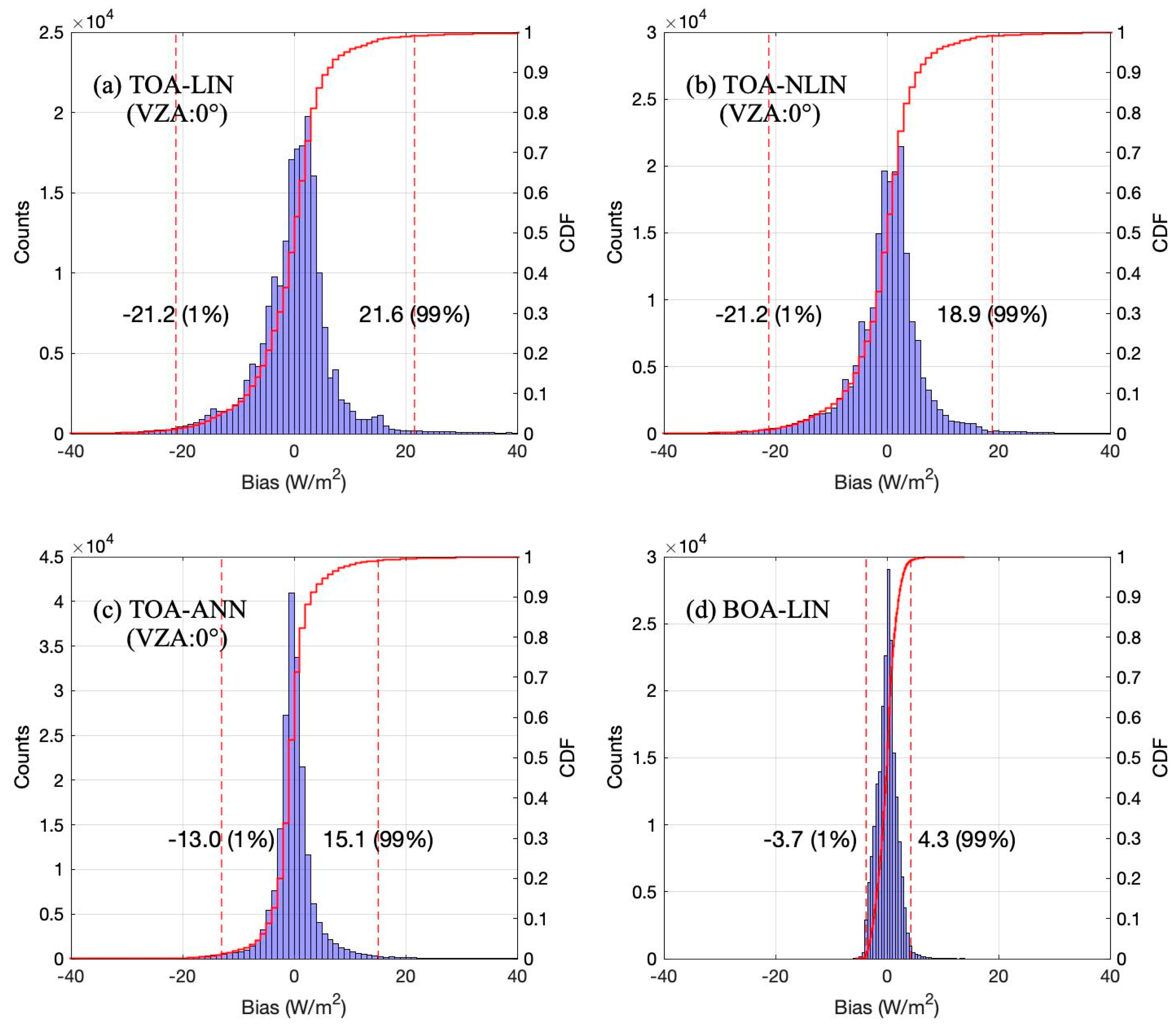
The bias histograms and CDFs (Cumulative Distribution Functions) for the four hybrid methods are shown in Figure 4. It should be noted that the binsize for TOA hybrid methods is 1 W/m2 and that for BOA-LIN is 0.5 W/m2. The bias histograms of all hybrid methods showed a normal distribution which centered at about 0 W/m2. Taking the bias values with CDF = 1% and CDF = 99% to indicate the bias level, we can see that the bias range for the BOA-LIN (−3.7 to 4.3 W/m2) is much smaller than that of TOA-LIN (−21.2 to 21.6 W/m2), TOA-NLIN (−21.2 to 18.9 W/m2), and TOA-ANN (−13.0 to 15.1 W/m2).
Using accurate atmospheric parameters ( L , i and   τ i ) the BOA linear hybrid method achieved a better theoretical accuracy than the other three hybrid methods in Figure 3 and Figure 4. However, the atmospheric parameters are sensitive to the wv [48,49,50], which is one of the most temporally and spatially dynamic variables in the atmosphere. To better understand the influence of wv accuracy in the SULR estimation of the BOA-LIN method, additional simulation analysis with two levels of wv errors were taken. The wv in the 946 TIGR atmosphere profiles were scaled with the number of 0.95 and 1.05 (0.9 and 1.1) to calculate the biased atmospheric parameters for the evaluation of the performance of BOA-LIN with a 5% (10%) wv error. It should be noted that the estimation accuracy of the BOA-LIN method under certain wv error (e.g., 5% or 10%) is also VZA dependent as shown in Table 7. This is because with the increase of the VZA, the optical path increases and thus the accuracy of the MODTRAN calculated atmospheric parameters (τ, L and L) decreases.
The results of BOA-LIN with accurate wv, 5% wv error (BOA-LIN_5%), and 10% wv error (BOA-LIN_10%), as well as the other three TOA hybrid methods from 0° to 60° are listed in Table 7. It can be seen that the TOA-LIN, BOA-LIN_5%, and BOA-LIN_10% have a larger RMSE and bias range with an increase of VZA. However, the results of VZA 10–60° are only evident for TOA-NLIN and TOA-ANN because of their nonlinearity. The BOA-LIN with no added wv error has a very small RMSE (1.75 W/m2) for all VZA values as expected. The RMSE of BOA-LIN_5% and BOA-LIN_10% increase sharply with the increase in VZA. All methods have a small MBE (<0.37 W/m2) and a high R2 (>0.993). Considering the mean RMSE values of all methods in Table 7, the performance in descending order is BOA-LIN, BOA-LIN_5%, TOA-ANN, TOA-NLIN, BOA- LIN_10%, and TOA-LIN.

4.2. Results and Analysis Based on In Situ Measurements

The evaluation results for all the six methods (TE-MYD11, TE-MYD21, TOA-LIN, TOA-NLIN, TOA-ANN, and BOA-LIN) using MODIS and in situ measurements (Section 2.2) are presented. The performances for all clear-sky data, daytime/night-time data, and each SURFRAD site are given in Section 4.2.1, Section 4.2.2, and Section 4.2.3, respectively. Section 4.2.4 and Section 4.2.5 compared the two temperature-emissivity methods and four hybrid methods, respectively. Finally, the comparison of the best physical method and hybrid method is presented in Section 4.2.6.

4.2.1. Six Methods Comparison for All Clear-Sky Data

The evaluation results of the six methods over all seven SURFRAD sites are shown in Figure 5. Their RMSE ranges from 14.0 W/m2 to 21.2 W/m2, MBE ranges from −0.2 W/m2 to −8.6 W/m2. The TE-MYD21 method performed the best with a RMSE of 14.0 W/m2 and MBE of −0.2 W/m2. However, the accuracy of the TE-MYD11 method ranks fifth with a RMSE of 18.5 W/m2 and MBE of −8.6 W/m2. The BOA-LIN method performs the best among the four hybrid methods with a RMSE of 15.2 W/m2 and MBE of −2.3 W/m2 as theoretical analysis based on the simulation dataset (Table 7) and proves the importance of taking the atmospheric correction into consideration. The TOA-NLIN method (with a RSME of 16.1 W/m2 and MBE of −4.6 W/m2) performs slightly better than the TOA-LIN method (with a RSME of 17.2 W/m2 and MBE of −5.5 W/m2). However, the TOA-ANN method (with a RSME of 21.2 W/m2 and MBE of −2.5 W/m2) performed the worst among all six methods which is contrary to the result shown in Table 6. Figure 5e shows that TOA-ANN has significant underestimation when SULR > 600 W/m2, probably due to the overfitting of the ANN structure.

4.2.2. Six Methods Comparison for Daytime and Night-Time Data

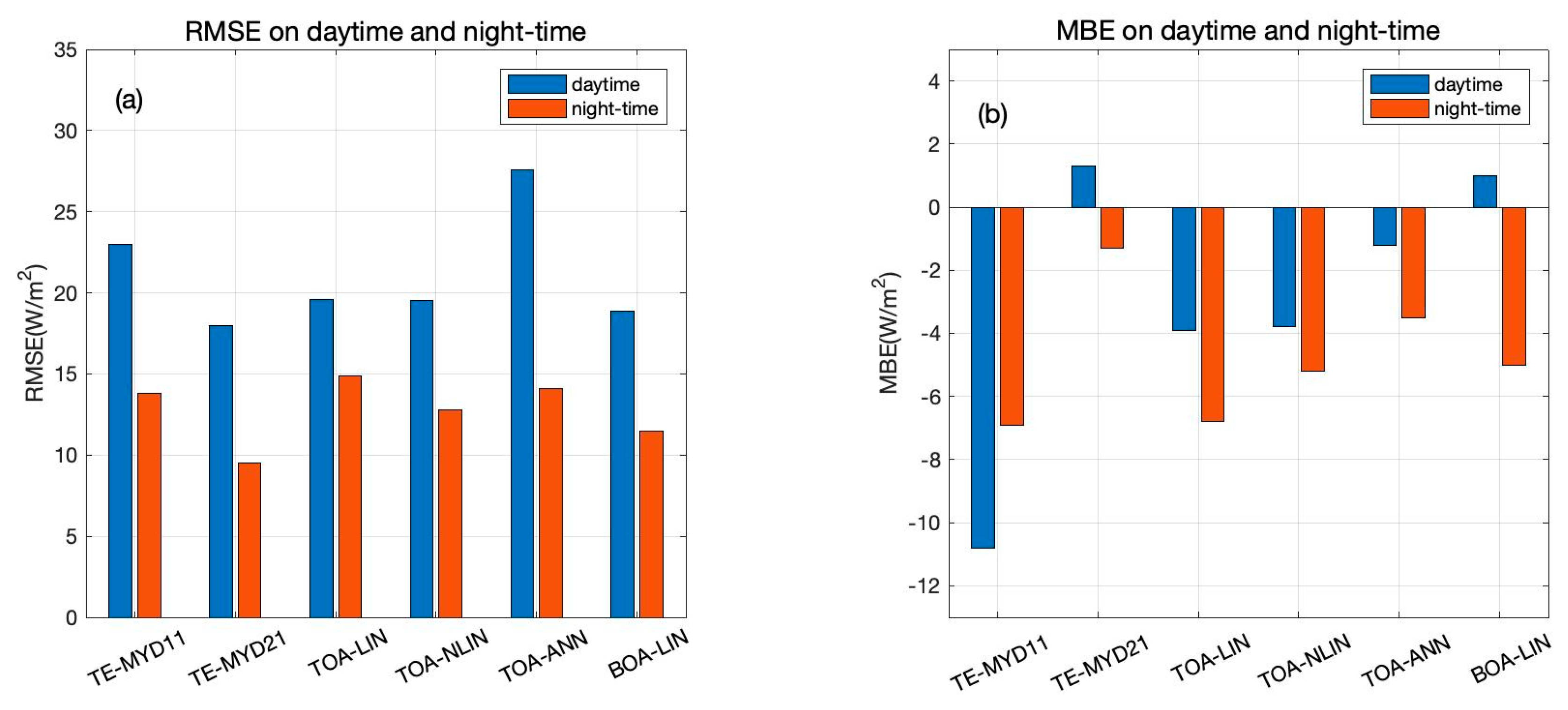
The validation results are separated for daytime and night-time as shown in Figure 6. The numbers of available in situ measurement clear-sky pixel for the daytime and night-time are 1422 and 1775, respectively. As we can see from the Figure 6a, the RMSE values in the daytime for all the six methods are greater than those in the night-time. The averaged RMSE (MBE) over the six methods in the daytime and night-time are 21.1 (−2.9) W/m2 and 12.8 (−4.7) W/m2, respectively. The higher RMSE in the daytime can be explained by the larger SULR variation range in the daytime (with SULR standard derivation value of 103 W/m2 in the daytime and 53 W/m2 in the night-time) and significant thermal radiation directionality (TRD) in the daytime [22,51].
The RMSE values for the daytime range from 18.0 W/m2 to 27.6 W/m2 and from 9.5 W/m2 to 14.9 W/m2 during the night-time. As seen in Figure 5, the TE-MYD21 performs the best among all the six methods (RMSE = 18.0 W/m2 in daytime and RMSE = 9.5 W/m2 in night-time) and the BOA-LIN (RMSE = 18.9 W/m2 in the daytime and RMSE = 11.5 W/m2 in the night-time) perform the best among all the four hybrid methods. In addition, the TOA-NLIN performs marginally better than the TOA-LIN in both night-time and daytime. The RMSE values for TE-MYD11, TOA-LIN, TOA-NLIN, and TOA-ANN during daytime (night-time) are 23.0 (13.8) W/m2, 19.6 (14.9) W/m2, 19.5 (12.8) W/m2, and 27.6 (14.1) W/m2, respectively.
The MBE in the daytime ranges from −10.8 W/m2 to 1.3 W/m2 and from −6.9 W/m2 to −1.3 W/m2 in the night-time. The TE-MYD21 and BOA-LIN have a positive MBE in the daytime with the value of 1.3 W/m2 and 1.0 W/m2 and a negative MBE in the night-time with the value of −1.3 W/m2 and −5.0 W/m2, respectively. The TE-MYD11 method has the most biased MBE with the value of −10.8 W/m2 and −6.9 W/m2 for both daytime and night-time. All the three TOA hybrid method shows a similar MBE pattern with an MBE closer to 0 in the daytime than that in the night-time. The MBE in daytime(night-time) for the TOA-ANN, TOA-NLIN and TOA-LIN are −1.2 W/m2 (−3.5 W/m2), −3.8 W/m2 (−5.2 W/m2), and −3.9 W/m2 (−6.8 W/m2), respectively.

4.2.3. Six Methods Comparison for Each Site

The RMSE and MBE values for all six methods over seven SURFRAD sites are listed in Table 8. The accuracy varies for different observation sites. In general, the results over FPE and PSU are the best. The RMSE of SXF, BOU, GCR, and BON are in the middle, and the result of DRA is the worst. The DRA site has an obvious negative bias (from −8.8 W/m2 to −25.3 W/m2) and a relatively high RMSE (from 15.9 W/m2 to 33.1 W/m2) which is similar to the previous studies of Wang et al. [13] and Cheng et al. [3]. The performance at the DRA site for TE-MYD21 (RMSE = 15.9 W/m2 and MBE = −8.8 W/m2) and BOA-LIN (RMSE = 17.5 W/m2 and MBE = −11.3 W/m2) is much better than the four remaining methods. This may be due to more accurate LST values from the MYD21 product over barren surfaces compared with the MYD11 product [52,53] and the accurate atmospheric correction in the BOA-LIN method, respectively.

4.2.4. The Intercomparison of Two Temperature-Emissivity Methods

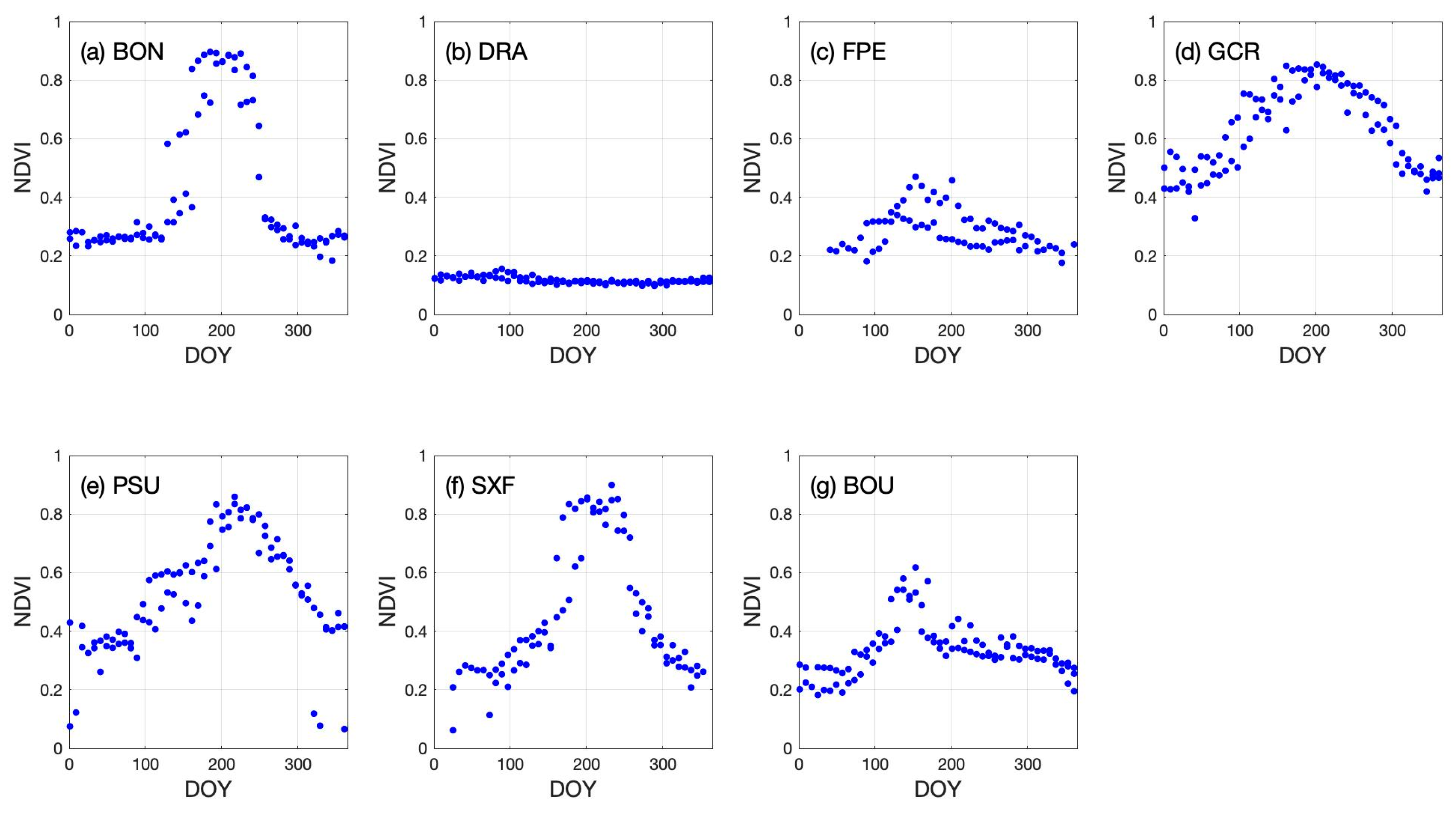
The TE-MYD11 and TE-MYD21 method use the same algorithm and same source of in situ measured DLR but different source of LST and LSE as described in Section 3.1. The significant improvement of TE-MYD21 method over DRA barren site has been discussed in Section 4.2.3. The performances of TE-MYD21 and TE-MYD11 over barren and non-barren surfaces are further analyzed at each site, considering that the non-barren sites (sites except DRA) will perform like barren in some seasons because of the vegetation annual growth cycle or man’s activities (e.g., tillage practices on cropland). The NDVI data at the seven SURFRAD sites is retrieved from the MODIS products (MOD13A2 and MYD13A2, 16-day composed with 1 km resolution) and used to describe the richness of vegetation. The retrieved NDVI values are shown in Figure 7; the x-axis is Day of Year (DOY) in 2017 and 2018. We can see that the NDVI values of the six vegetated SURFRAD sites (BON, FPE, GCR, PSU, SXF, and BOU) have obvious annual cycles, while the desert site (DRA) has a very low and stable NDVI value. For BON, GCR, PSU, and SXF sites, the NDVI reached the highest value (>0.8) at about DOY 210 (end of July). For FPE and BOU, the NDVI reached the highest value (<0.62) at about DOY 153 (early June). The DRA shows a relatively constant NDVI at about 0.12.
The land surfaces with NDVI lower than 0.3 is recognized as barren surfaces in this study. The percentage and mean NDVI of barren and non-barren observations at the seven SURFRAD sites and corresponding MBEs and RMSEs for the TE-MYD21 and TE-MYD11 methods are summarized in Table 9. The available observations are all barren (NDVI < 0.3) for DRA site and are all non-barren (NDVI ≥ 0.3) for GCR and PSU sites. For barren surfaces, the TE-MYE21 performs better than the TE-MYD11 method at four sites (DRA, FPE, SXF, and BOU) among five available sites and the weighted mean RMSE (MBE) are 14.2 W/m2 (−4.2 W/m2) and 22.4 W/m2 (−14.9 W/m2) for TE-MYD21 and TE-MYD11 methods. For non-barren surfaces, the TE-MYE11 performs slightly better than the TE-MYD21 method at four sites (BON, PSU, SXF, and BOU) among six available sites and the weighted mean RMSE (MBE) are 13.8 W/m2 (3.7 W/m2) and 13.6 W/m2 (−2.5 W/m2) for TE-MYD21 and TE-MYD11 methods. The TE-MYD21 shows a much better accuracy than TE-MYD11 method at barren surfaces and a similar accuracy at non-barren surfaces.

4.2.5. The Intercomparison of Four Hybrid Methods

The TOA hybrid methods only require TOA radiances and coefficients when calculating the SULR, while the BOA-LIN method needs additional inputs of atmospheric profiles for atmospheric correction. The performance of the BOA-LIN method highly depends on the wv accuracy of the atmospheric profile as shown in Table 6. In this section, the RMSE values of four hybrid methods with different wv values (step = 0.5) are compared.
The wv histogram (Figure 8a) shows that 93.0% of the observations have a wv in the range of [0, 4]g/cm2. The observations with wv > 4.0 g/m2 are not considered here because of the low frequency. The RMSE comparison of four hybrid methods at different wv are shown in Figure 8b. It can be seen that the BOA-LIN method has the lowest RMSE for wv < 3 g/m2 and a relatively small RMSE for 3 g/m2 < wv < 4 g/m2. The TOA-ANN has the largest RMSE for wv > 1 g/cm2. The TOA-LIN and TOA-NLIN show an intermediate accuracy and the later one is more accurate for wv < 2 g/cm2. The MBE comparison of four hybrid methods at different wv are shown in Figure 8c. The BOA-LIN method has the most stable MBE likely due to the step of atmospheric correction. The TOA-ANN method has the most variable MBE maybe due to the over fitting of the ANN-structure. TOA-NLIN method has a MBE closer to zero than the TOA-LIN for wv < 2 g/cm2 similar to the RMSE.

4.2.6. The Comparison of TE-MYD21 and BOA-LIN

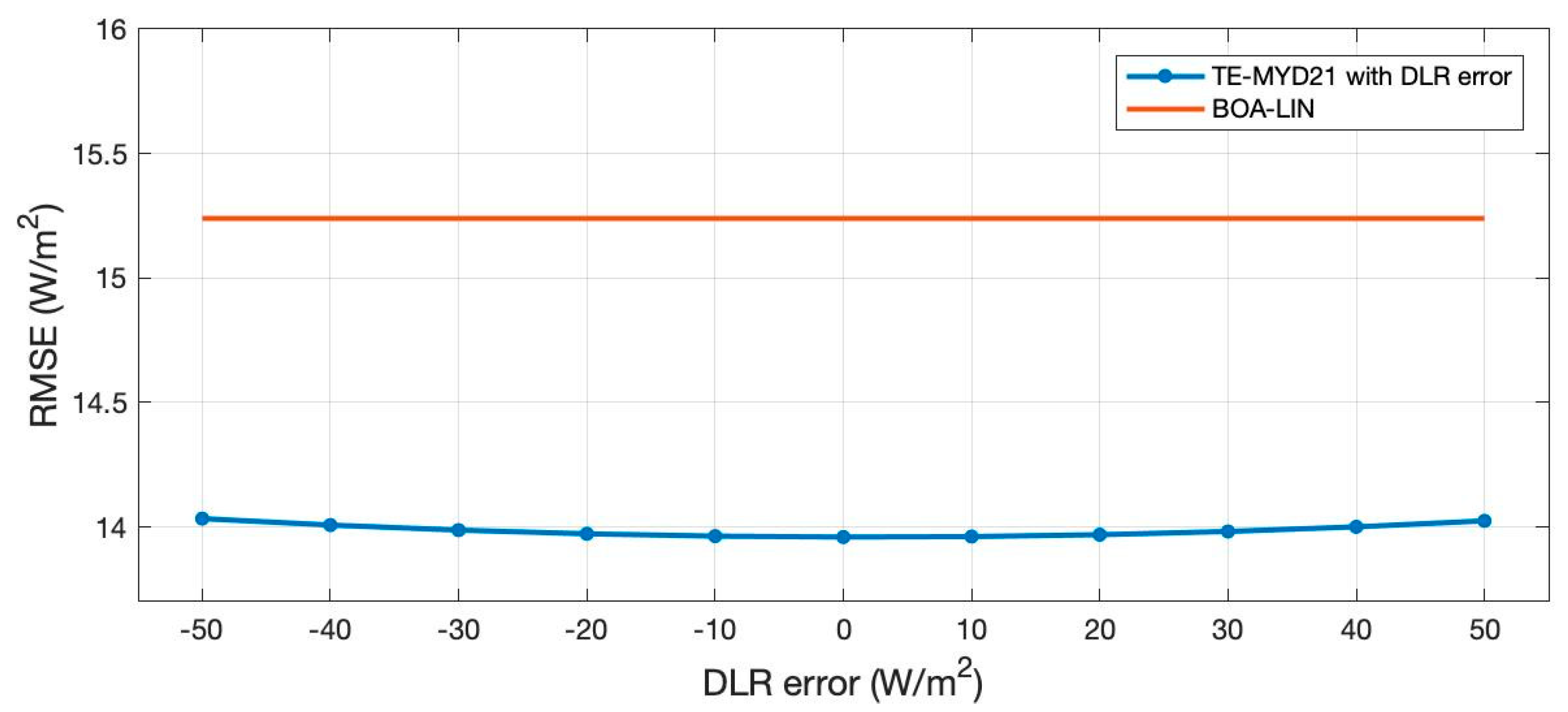
The TE-MYD21 and BOA-LIN are shown to be the best methods in their respective categories while the TE-MYD21 performed slightly better than the BOA-LIN method (see Table 8). The DLR used in TE-MYD21 was in situ measured data however in the global SULR generation, the DLR is usually obtained from remote sensing or reanalysis products. It is reported that the DLR estimation can achieve an accuracy of ~25 W/m2 [4,48]. The RMSE of TE-MYD21 method with varying DLR errors were compared with RMSE of BOA-LIN in Figure 9. A 50 W/m2 bias of DLR leads to a <0.074 W/m2 bias to the RMSE of the TE-MYD21. Therefore, the TE-MYD21 method likely performs better than the BOA-LIN in applications. Nevertheless, the BOA-LIN method is also a good choice for the satellite sensors that cannot utilize the TES algorithm to estimate accurate LST and LSE.

5. Conclusions

This paper evaluated six clear-sky SULR estimation methods with simulation datasets and Aqua-MODIS measurements. The recently released MYD21 product was used to estimate the SULR. A new method (BOA-LIN) was developed under the general framework of the hybrid method but also includes atmospheric correction to eliminate the effect of atmosphere. Some of the new insights into the SULR estimation methods are as follows.
(1)
For the theoretical analysis of TOA hybrid methods (TOA-LIN, TOA-NLIN, TOA-ANN), the fitting RMSE decreases with increasing model nonlinearity. The fitting RMSE of BOA-LIN (1.75 W/m2) is much less than the RMSE of the TOA hybrid methods assuming an accurate atmospheric correction has been achieved. The performance of BOA-LIN decays with the increase of atmospheric profile wv error. The BOA hybrid method has great potential in application if accurate atmospheric profiles can be obtained as input.
(2)
The TE-MYD21 performs the best among all the six methods with RMSE of 14.0 W/m2 and MBE of −0.2 W/m2, and the BOA-LIN performs best among the four hybrid methods with RMSE of 15.2 W/m2 and MBE of −2.3 W/m2 based on the two-year satellite products. The performance of six methods in descending order is TE-MYD21, BOA-LIN, TOA-NLIN, TOA-LIN, TE-MYD11, and TOA-ANN. TE-MYD21 has a much better accuracy than the TE-MYD11 over barren surfaces (NDVI < 0.3) and a similar accuracy over non-barren surfaces (NDVI ≥ 0.3). The BOA-LIN is more accurate than other TOA hybrid methods due to the inclusion of atmospheric correction.
SULR is an important parameter in the estimation of the radiation budget that needs to be estimated accurately with remotely sensed data. More adequate evaluation is needed in the future with more spatial locations and longer temporal coverage. All six SULR estimation methods presented here are under the thermal isotropic assumption because MODIS can only supply one viewing angle observation. Further studies should focus on the development of SULR calculation methods that take into consideration the thermal directionality.

Author Contributions

Conceptualization, B.Q.; Data curation, B.Q., H.L., Z.B., and T.H.; Formal analysis, H.L., Z.B., and T.H.; Funding acquisition, B.C., Q.X., and Q.L.; Investigation, B.Q. and B.C.; Methodology, B.Q. and B.C.; Resources, B.C., H.L., Y.D., and Y.Y.; Software, B.Q. and Y.Y.; Validation, B.Q.; Writing—original draft, B.Q.; Writing—review & editing, B.C., Z.B., T.H., Y.D., Q.X., and Q.L. All authors have read and agreed to the published version of the manuscript.

Funding

This work was supported in part by the National Key Research and Development Program of China under Grant 2018YFA0605503; in part by the National Natural Science of Foundation of China under Grant 41871258, Grant 41930111; in part by the Strategic Priority Research Program of Chinese Academy of Sciences under Grant XDA15012400; in part by the National Natural Science of Foundation of China under Grant 41901287, and Grant 41671366; in part by the Youth Innovation Promotion Association CAS under Grant 2020127; in part by the “Future Star” Talent Plan of the Aerospace Information Research Institute of Chinese Academy of Sciences under Grant Y920570Z1F; and in part by the Director Foundation of the Institute of Remote Sensing and Digital Earth of Chinese Academy of Sciences under Grant Y5SJ1300CX.

Conflicts of Interest

The authors declare no conflicts of interest.

References

  1. Gupta, S.K.; Ritchey, N.A.; Wilber, A.C.; Whitlock, C.H.; Gibson, G.G.; Stackhouse, P.W., Jr. A climatology of surface radiation budget derived from satellite data. J. Clim. 1999, 12, 2691–2710. [Google Scholar] [CrossRef]
  2. Liang, S.; Wang, K.; Zhang, X.; Wild, M. Review on Estimation of Land Surface Radiation and Energy Budgets From Ground Measurement, Remote Sensing and Model Simulations. IEEE J. Sel. Top. Appl. Earth Obs. Remote Sens. 2010, 3, 225–240. [Google Scholar] [CrossRef]
  3. Cheng, J.; Liang, S. Global Estimates for High-Spatial-Resolution Clear-Sky Land Surface Upwelling Longwave Radiation From MODIS Data. IEEE Trans. Geosci. Remote Sens. 2016, 54, 4115–4129. [Google Scholar] [CrossRef]
  4. Wang, W.; Liang, S. Estimation of high-spatial resolution clear-sky longwave downward and net radiation over land surfaces from MODIS data. Remote Sens. Environ. 2009, 113, 745–754. [Google Scholar] [CrossRef]
  5. Yang, J.; Gong, P.; Fu, R.; Zhang, M.; Chen, J.; Liang, S.; Xu, B.; Shi, J.; Dickinson, R. The role of satellite remote sensing in climate change studies. Nat. Clim. Chang. 2013, 3, 875–883. [Google Scholar] [CrossRef]
  6. Weng, Q. Thermal infrared remote sensing for urban climate and environmental studies: Methods, applications, and trends. ISPRS J. Photogramm. Remote Sens. 2009, 64, 335–344. [Google Scholar] [CrossRef]
  7. Wielicki, B.A.; Barkstrom, B.R.; Baum, B.A.; Charlock, T.P.; Green, R.N.; Kratz, D.P.; Lee, R.B.; Minnis, P.; Smith, G.L.; Wong, T. Clouds and the Earth’s Radiant Energy System (CERES): Algorithm overview. IEEE Trans. Geosci. Remote Sens. 1998, 36, 1127–1141. [Google Scholar] [CrossRef] [Green Version]
  8. Yan, H.; Huang, J.; Minnis, P.; Wang, T.; Bi, J. Comparison of CERES surface radiation fluxes with surface observations over Loess Plateau. Remote Sens. Environ. 2011, 115, 1489–1500. [Google Scholar] [CrossRef] [Green Version]
  9. Liang, S.; Wang, D.; He, T.; Yu, Y. Remote sensing of earth’s energy budget: Synthesis and review. Int. J. Digit. Earth 2019, 12, 737–780. [Google Scholar] [CrossRef] [Green Version]
  10. Wielicki, B.A.; Barkstrom, B.R.; Harrison, E.F.; Lee, R.B.; Louis Smith, G.; Cooper, J.E. Clouds and the Earth’s Radiant Energy System (CERES): An Earth Observing System Experiment. Bull. Am. Meteorol. Soc. 1996, 77, 853–868. [Google Scholar] [CrossRef] [Green Version]
  11. Bisht, G.; Venturini, V.; Islam, S.; Jiang, L. Estimation of the net radiation using MODIS (Moderate Resolution Imaging Spectroradiometer) data for clear sky days. Remote Sens. Environ. 2005, 97, 52–67. [Google Scholar] [CrossRef]
  12. Tang, B.; Li, Z.-L. Estimation of instantaneous net surface longwave radiation from MODIS cloud-free data. Remote Sens. Environ. 2008, 112, 3482–3492. [Google Scholar] [CrossRef]
  13. Wang, W.; Liang, S.; Augustine, J.A. Estimating High Spatial Resolution Clear-Sky Land Surface Upwelling Longwave Radiation From MODIS Data. IEEE Trans. Geosci. Remote Sens. 2009, 47, 1559–1570. [Google Scholar] [CrossRef]
  14. Gillespie, A.; Rokugawa, S.; Matsunaga, T.; Cothern, J.S.; Hook, S.; Kahle, A.B. A temperature and emissivity separation algorithm for Advanced Spaceborne Thermal Emission and Reflection Radiometer (ASTER) images. IEEE Trans. Geosci. Remote Sens. 1998, 36, 1113–1126. [Google Scholar] [CrossRef]
  15. Wan, Z.; Dozier, J. A generalized split-window algorithm for retrieving land-surface temperature from space. IEEE Trans. Geosci. Remote Sens. 1996, 34, 892–905. [Google Scholar]
  16. Snyder, W.C.; Wan, Z.; Zhang, Y.; Feng, Y.-Z. Classification-based emissivity for land surface temperature measurement from space. Int. J. Remote Sens. 1998, 19, 2753–2774. [Google Scholar] [CrossRef]
  17. Wu, H.; Zhang, X.; Liang, S.; Yang, H.; Zhou, G. Estimation of clear-sky land surface longwave radiation from MODIS data products by merging multiple models. J. Geophys. Res. Atmos. 2012, 117. [Google Scholar] [CrossRef]
  18. Wang, T.; Yan, G.; Chen, L. Consistent retrieval methods to estimate land surface shortwave and longwave radiative flux components under clear-sky conditions. Remote Sens. Environ. 2012, 124, 61–71. [Google Scholar] [CrossRef]
  19. Wang, C.; Tang, B.H.; Huo, X.; Li, Z.L. New method to estimate surface upwelling long-wave radiation from MODIS cloud-free data. Opt. Express 2017, 25, A574–A588. [Google Scholar] [CrossRef]
  20. Jiao, Z.; Yan, G.; Zhao, J.; Wang, T.; Chen, L. Estimation of surface upward longwave radiation from MODIS and VIIRS clear-sky data in the Tibetan Plateau. Remote Sens. Environ. 2015, 162, 221–237. [Google Scholar] [CrossRef]
  21. Cao, B.; Liu, Q.; Du, Y.; Roujean, J.-L.; Gastellu-Etchegorry, J.-P.; Trigo, I.F.; Zhan, W.; Yu, Y.; Cheng, J.; Jacob, F. A review of earth surface thermal radiation directionality observing and modeling: Historical development, current status and perspectives. Remote Sens. Environ. 2019, 232, 111304. [Google Scholar] [CrossRef]
  22. Hu, T.; Cao, B.; Du, Y.; Li, H.; Wang, C.; Bian, Z.; Sun, D.; Liu, Q. Estimation of surface upward longwave radiation using a direct physical algorithm. IEEE Trans. Geosci. Remote Sens. 2017, 55, 4412–4426. [Google Scholar] [CrossRef]
  23. Chedin, A.; Scott, N.; Wahiche, C.; Moulinier, P. The improved initialization inversion method: A high resolution physical method for temperature retrievals from satellites of the TIROS-N series. J. Clim. Appl. Meteorol. 1985, 24, 128–143. [Google Scholar] [CrossRef] [Green Version]
  24. Chevallier, F.; Chéruy, F.; Scott, N.A.; Chédin, A. A Neural Network Approach for a Fast and Accurate Computation of a Longwave Radiative Budget. J. Appl. Meteorol. 1998, 37, 1385–1397. [Google Scholar] [CrossRef]
  25. Ren, H.; Du, C.; Liu, R.; Qin, Q.; Yan, G.; Li, Z.L.; Meng, J. Atmospheric water vapor retrieval from Landsat 8 thermal infrared images. J. Geophys. Res. Atmos. 2015, 120, 1723–1738. [Google Scholar] [CrossRef]
  26. Ye, X.; Ren, H.; Liu, R.; Qin, Q.; Liu, Y.; Dong, J. Land surface temperature estimate from chinese gaofen-5 satellite data using split-window algorithm. IEEE Trans. Geosci. Remote Sens. 2017, 55, 5877–5888. [Google Scholar] [CrossRef]
  27. Li, Z.-L.; Wu, H.; Wang, N.; Qiu, S.; Sobrino, J.A.; Wan, Z.; Tang, B.-H.; Yan, G. Land surface emissivity retrieval from satellite data. Int. J. Remote Sens. 2013, 34, 3084–3127. [Google Scholar] [CrossRef]
  28. Wang, K.; Wan, Z.; Wang, P.; Sparrow, M.; Liu, J.; Zhou, X.; Haginoya, S. Estimation of surface long wave radiation and broadband emissivity using Moderate Resolution Imaging Spectroradiometer (MODIS) land surface temperature/emissivity products. J. Geophys. Res. Atmos. 2005, 110. [Google Scholar] [CrossRef]
  29. Berk, A.; Anderson, G.; Acharya, P.; Hoke, M.; Chetwynd, J.; Bernstein, L.; Shettle, E.; Matthew, M.; Adler-Golden, S. MODTRAN4 version 3 revision 1 user’s manual. Air Force Res. Lab. Space Veh. Dir. Air Force Mater. Command AFB MA 2003, 1731, 3010. [Google Scholar]
  30. Rodriguez, E.; Morris, C.S.; Belz, J.E. A global assessment of the SRTM performance. Photogramm. Eng. Remote Sens. 2006, 72, 249–260. [Google Scholar] [CrossRef] [Green Version]
  31. Li, H.; Liu, Q.; Du, Y.; Jiang, J.; Wang, H. Evaluation of the NCEP and MODIS Atmospheric Products for Single Channel Land Surface Temperature Retrieval With Ground Measurements: A Case Study of HJ-1B IRS Data. IEEE J. Sel. Top. Appl. Earth Obs. Remote Sens. 2013, 6, 1399–1408. [Google Scholar] [CrossRef]
  32. Meng, X.; Cheng, J. Evaluating Eight Global Reanalysis Products for Atmospheric Correction of Thermal Infrared Sensor—Application to Landsat 8 TIRS10 Data. Remote Sens. 2018, 10, 474. [Google Scholar] [CrossRef] [Green Version]
  33. Augustine, J.A.; Hodges, G.B.; Cornwall, C.R.; Michalsky, J.J.; Medina, C.I. An Update on SURFRAD—The GCOS Surface Radiation Budget Network for the Continental United States. J. Atmos. Ocean. Technol. 2005, 22, 1460–1472. [Google Scholar] [CrossRef]
  34. Philipona, R.; Fröhlich, C.; Dehne, K.; DeLuisi, J.; Augustine, J.; Dutton, E.; Nelson, D.; Forgan, B.; Novotny, P.; Hickey, J. The Baseline Surface Radiation Network pyrgeometer round-robin calibration experiment. J. Atmos. Ocean. Technol. 1998, 15, 687–696. [Google Scholar] [CrossRef]
  35. Wan, Z.; Zhang, Y.; Zhang, Q.; Li, Z.L. Validation of the land-surface temperature products retrieved from Terra Moderate Resolution Imaging Spectroradiometer data. Remote Sens. Environ. 2002, 83, 163–180. [Google Scholar] [CrossRef]
  36. Wan, Z.; Zhang, Y.; Zhang, Q.; Li, Z.L. Quality assessment and validation of the MODIS global land surface temperature. Int. J. Remote Sens. 2010, 25, 261–274. [Google Scholar] [CrossRef]
  37. Wan, Z. New refinements and validation of the collection-6 MODIS land-surface temperature/emissivity product. Remote Sens. Environ. 2014, 140, 36–45. [Google Scholar] [CrossRef]
  38. Wan, Z.; Li, Z.-L. A physics-based algorithm for retrieving land-surface emissivity and temperature from EOS/MODIS data. IEEE Trans. Geosci. Remote Sens. 1997, 35, 980–996. [Google Scholar]
  39. Li, Z.-L.; Becker, F. Feasibility of land surface temperature and emissivity determination from AVHRR data. Remote Sens. Environ. 1993, 43, 67–85. [Google Scholar] [CrossRef]
  40. Tonooka, H. Accurate atmospheric correction of ASTER thermal infrared imagery using the WVS method. IEEE Trans. Geosci. Remote Sens. 2005, 43, 2778–2792. [Google Scholar] [CrossRef]
  41. Hulley, G.C.; Hughes, C.G.; Hook, S.J. Quantifying uncertainties in land surface temperature and emissivity retrievals from ASTER and MODIS thermal infrared data. J. Geophys. Res. Atmos. 2012, 117. [Google Scholar] [CrossRef] [Green Version]
  42. Hulley, G.; Veraverbeke, S.; Hook, S. Thermal-based techniques for land cover change detection using a new dynamic MODIS multispectral emissivity product (MOD21). Remote Sens. Environ. 2014, 140, 755–765. [Google Scholar] [CrossRef]
  43. Lee, H.-T.; Ellingson, R.G. Development of a Nonlinear Statistical Method for Estimating the Downward Longwave Radiation at the Surface from Satellite Observations. J. Atmos. Ocean. Technol. 2002, 19, 1500–1515. [Google Scholar] [CrossRef] [Green Version]
  44. Mao, K.; Tang, H.; Wang, X.; Zhou, Q.; Wang, D. Near-surface air temperature estimation from ASTER data based on neural network algorithm. Int. J. Remote Sens. 2008, 29, 6021–6028. [Google Scholar] [CrossRef]
  45. Ahmad, S.; Kalra, A.; Stephen, H. Estimating soil moisture using remote sensing data: A machine learning approach. Adv. Water Resour. 2010, 33, 69–80. [Google Scholar] [CrossRef]
  46. Walthall, C.; Dulaney, W.; Anderson, M.; Norman, J.; Fang, H.; Liang, S. A comparison of empirical and neural network approaches for estimating corn and soybean leaf area index from Landsat ETM+ imagery. Remote Sens. Environ. 2004, 92, 465–474. [Google Scholar] [CrossRef]
  47. Hornik, K.; Stinchcombe, M.; White, H. Multilayer feedforward networks are universal approximators. Neural Netw. 1989, 2, 359–366. [Google Scholar] [CrossRef]
  48. Cheng, J.; Liang, S.; Wang, W.; Guo, Y. An efficient hybrid method for estimating clear-sky surface downward longwave radiation from MODIS data. J. Geophys. Res. Atmos. 2017, 122, 2616–2630. [Google Scholar] [CrossRef]
  49. Jiménez-Muñoz, J.C.; Sobrino, J.A. A generalized single-channel method for retrieving land surface temperature from remote sensing data. J. Geophys. Res. Atmos. 2003, 108. [Google Scholar] [CrossRef] [Green Version]
  50. Qin, Z.; Karnieli, A.; Berliner, P. A mono-window algorithm for retrieving land surface temperature from Landsat TM data and its application to the Israel-Egypt border region. Int. J. Remote Sens. 2010, 22, 3719–3746. [Google Scholar] [CrossRef]
  51. Hu, T.; Du, Y.; Cao, B.; Li, H.; Bian, Z.; Sun, D.; Liu, Q. Estimation of Upward Longwave Radiation From Vegetated Surfaces Considering Thermal Directionality. IEEE Trans. Geosci. Remote Sens. 2016, 54, 6644–6658. [Google Scholar] [CrossRef]
  52. Li, H.; Li, R.; Yang, Y.; Cao, B.; Bian, Z.; Hu, T.; Du, Y.; Sun, L.; Liu, Q. Temperature-based and Radiance-based Validation of the Collection 6 MYD11 and MYD21 Land Surface Temperature Products Over Barren Surfaces in Northwestern China. IEEE Trans. Geosci. Remote Sens. (in press).
  53. Li, H.; Sun, D.L.; Yu, Y.Y.; Wang, H.Y.; Liu, Y.L.; Liu, Q.H.; Du, Y.M.; Wang, H.S.; Cao, B.A. Evaluation of the VIIRS and MODIS LST products in an arid area of Northwest China. Remote Sens. Environ. 2014, 142, 111–121. [Google Scholar] [CrossRef] [Green Version]
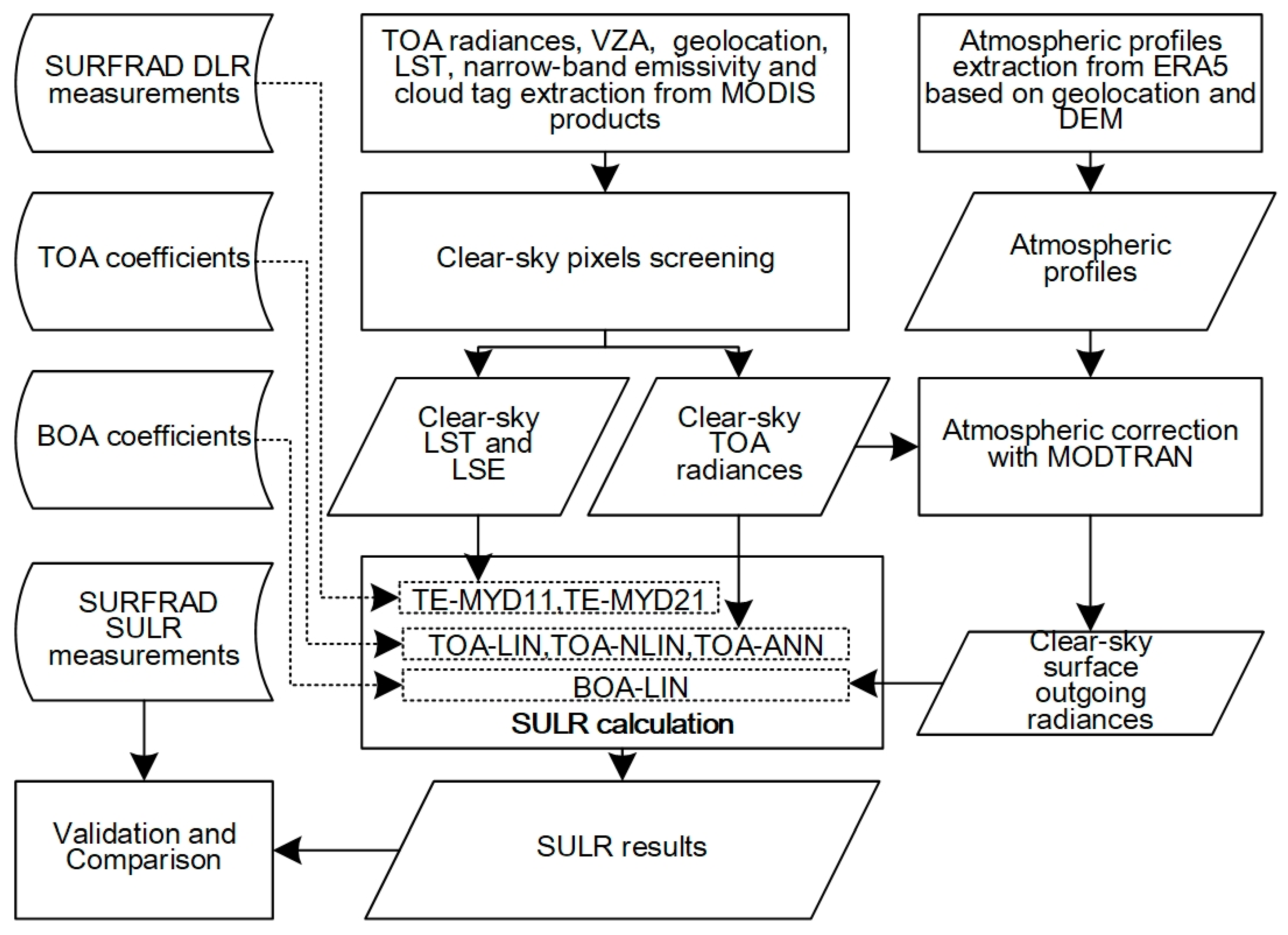
Figure 1. The flowchart of data processing for the Moderate Resolution Imaging Spectroradiometer (MODIS), ERA5, and in situ measurements.
Remotesensing 12 01834 g001
Figure 2. The flowchart of the coefficient estimation for the hybrid methods.
Remotesensing 12 01834 g002
Figure 3. Scatterplots between MODTRAN simulated SULR and estimated SULR of four hybrid methods (ac), TOA-LIN, TOA-NLIN, and TOA-ANN methods with simulation data of VZA = 0°. (d) BOA-LIN method with all VZA values.
Remotesensing 12 01834 g003
Figure 4. Statistical histograms and CDFs of SULR estimation bias (the red dotted lines indicate the bias values for CDF equal to 1% and 99%). (ac) For the TOA-LIN, TOA-NLIN, and TOA-ANN methods with simulation data of VZA = 0° with 1 W/m2 bin size. (d) For BOA-LIN methods with all VZA values with 0.5 W/m2 bin size.
Remotesensing 12 01834 g004
Figure 5. Scatterplots between estimated SULR and corresponding in situ SURFRAD measurement for all six methods. (a) TE-MYD11. (b) TE-MYD21. (c) TOA-LIN. (d) TOA-NLIN. (e) TOA-ANN. (f) BOA-LIN.
Remotesensing 12 01834 g005
Figure 6. Histograms for daytime and night-time RMSE and MBE of the in situ measurement data. (a) RMSE. (b) MBE.
Remotesensing 12 01834 g006
Figure 7. NDVI data for seven SURFRAD sites at the year of 2017 and 2018. (a) BON. (b) DRA. (c) FPE. (d) GCR. (e) PSU. (f) SXF. (g) BOU.
Remotesensing 12 01834 g007
Figure 8. The comparison of four hybrid methods. (a) The wv histogram of the clear-sky observations. (b) The RMSE comparison of four hybrid methods at different wv. (c) The MBE comparison of four hybrid methods at different wv.
Remotesensing 12 01834 g008
Figure 9. The accuracy comparison of BOA-LIN and TE-MYD21 method with DLR errors.
Remotesensing 12 01834 g009
Table 1. List of the MODIS products used in this study.
MODIS ProductsSpatial Resolution (km)Temporal ResolutionProducts Description
(Used Layers)
Model to Drive
MYD021KM1DailyTOA radiance acquired by Aqua
(Bands 29, 31 and 32 only)
Four hybrid methods
MYD031DailyLocations and ancillary information corresponding to the swath data of Aqua
(Latitude, Longitude and VZA)
All SULR methods
MYD35_L21DailyCloud mask and spectral test results corresponding to the swath data of Aqua
(Cloud mask)
All SULR methods
MYD11B15.6DailyLST&LSE generated with the day/night algorithm
(LSEs for bands 29, 31 and 32)
TE-MYD11
MYD11_L21DailyLST&LSE generated with the generalized split-window algorithm
(LSTs for bands 29, 31 and 32)
TE-MYD11
MYD21_L21DailyLST&LSE generated with the TES algorithm
(LST, LSE)
TE-MYD21
MOD13A2& MYD13A218-day with MOD&MYD combinedVegetation Index values
(NDVI)
-
Table 2. Validation sites of SURFRAD.
Station NameLatitude, LongitudeLand CoverElevation (m)Station ID
Bondville40.05192°N, 88.37309°W Cropland230BON
Desert Rock36.62373°N, 116.01947°W Open Shrubland1007DRA
Fort Peck48.30783°N, 105.10170°W Grassland634FPE
Goodwin Creek34.2547°N, 89.8729°W Cropland/natural vegetation mosaic98GCR
Penn. State Univ. 40.72012°N, 77.93085°W Cropland/natural vegetation mosaic 376PSU
Sioux Falls43.73403°N, 96.62328°W Grassland473SXF
Boulder40.12498°N, 105.23680°W Grassland1689BOU
Table 3. Coefficients of the TOA-LIN model with VZA = 0 ° 60 ° .
θ v   a 0     a 1     a 2     a 3  
  0 °   85.549−1.846132.003−95.882
  10 °   85.951−1.924133.113−97.023
  20 °   87.201−2.158136.524−100.536
  30 °   89.437−2.543142.488−106.704
  40 °   92.931−3.059151.479−116.076
  50 °   98.178−3.607164.247−129.571
  60 °   106.052−3.810181.853−148.694
Table 4. Coefficients of TOA-NLIN model at VZA 0 ° 60 ° .
θ v   k     c 1     c 2     c 3     c 4     b  
  0 °   36.424−18.3510.4620.8532.12137.823
  10 °   34.546−16.1850.4620.43514.87431.081
  20 °   33.621−15.9650.4640.4513.69530.254
  30 °   31.868−15.5020.4690.4801.62128.609
  40 °   33.587−14.0510.4590.5100.86025.582
  50 °   32.267−11.8130.4580.5720.51619.891
  60 °   30.139−7.1920.4520.6770.3208.273
Table 5. The structure and training parameters of the BPNN model used for each VZA.
θ v Network StructureInputOutputNumber of Epochs
  0 °   (3-7-1)Radiances of MODIS B29, 31, and 32 from the simulation datasetCorresponding SULR from the simulation dataset500
  10 °  
  20 °  
  30 °  
  40 °  
  50 °  
  60 °  
Table 6. Coefficients of BOA-LIN model.
a 0   a 1     a 2     a 3  
50.5287.7547.53229.540
Table 7. Comparison results for four hybrid methods based on simulation dataset (W/m2).
θ TOA-LINTOA-NLINTOA-ANNBOA-LIN
(No wv Error)
BOA-LIN_5%
(5% wv Error)
BOA-LIN_10%
(10% wv Error)
R2RMSE
&MBE
Bias
Range
R2RMSE
&MBE
Bias
Range
R2RMSE
&MBE
Bias
Range
R2RMSE
&MBE
Bias
Range
R2RMSE
&MBE
Bias
Range
R2RMSE
&MBE
Bias
Range
0.9957.37, 0.00−21.2, 21.60.9966.91, 0.00−21.2, 18.90.9984.46, 0.00−13.0, 15.10.99971.75, 0.00−3.7, 4.30.999 2.89, 0.01−8.3, 10.10.998 4.99, 0.14−14.3, 19.9
10°0.9957.43, 0.00−21.4, 21.90.9966.25, 0.00−23.3, 14.30.9984.44, 0.00−13.4, 13.90.999 2.93, 0.01−8.4, 10.30.998 5.09, 0.15−14.6, 20.3
20°0.9957.63, 0.00−21.9, 22.50.9966.37, 0.00−23.8, 14.50.9984.55, 0.00−13.6, 15.00.999 3.06, 0.01−8.8, 10.9 0.997 5.39, 0.17−15.4, 21.9
30°0.9947.99, 0.00−22.9, 23.80.9966.59, 0.00−24.8, 15.00.9984.76, 0.02−14.1, 15.70.999 3.31, 0.02−9.5, 12.00.997 6.01, 0.21−17.0, 24.5
40°0.9938.58, 0.00−24.1, 26.00.9966.96, 0.00−26.2, 16.00.9985.06, 0.01−14.4, 17.00.999 3.79, 0.30−11.0, 14.30.995 7.17, 0.30−19.6, 29.8
50°0.9929.54, 0.00−26.7, 29.80.9957.60, 0.00−28.3, 17.90.9975.46, 0.03−15.8, 18.40.998 4.81, 0.09−13.7, 18.80.992 9.63, 0.51−24.6, 40.8
60°0.98911.2, 0.00−30.4, 37.10.9938.82, 0.00−31.8, 22.20.9966.38, −0.01−17.6, 21.90.995 7.63, 0.25−20.4, 29.80.977 16.72, 1.13−36.2, 67.5
Mean0.9938.53, 0.00−24.1, 26.10.9957.07,0.00−25.6,17.00.9985.02, 0.01−14.6, 16.70.99971.75, 0.00−3.7, 4.30.9984.06, 0.01−11.4, 15.20.9937.86, 0.37−20.2, 32.1
Table 8. Summary of validation results for six methods over 7 SURFRAD sites (W/m2).
Site Name # of obsTE-MYD11TE-MYD21TOA-LINTOA-NLINTOA-ANNBOA-LIN
RMSE
&MBE
RMSE
&MBE
RMSE
&MBE
RMSE
&MBE
RMSE
&MBE
RMSE
&MBE
BON33613.9−0.117.17.115.73.314.93.016.46.718.45.0
DRA85528.8−25.315.9−8.825.5−22.422.7−18.733.1−24.217.5−11.3
FPE5389.9−3.59.21.29.3−0.710.00.411.74.210.3−0.7
GCR39316.8−6.014.12.114.2−0.714.5−1.814.83.614.7−0.5
PSU1849.00.811.77.310.32.89.72.613.58.812.54.8
SXF42611.9−1.013.63.912.81.413.01.215.05.514.22.0
BOU46512.8−2.913.10.213.8−0.214.1−0.316.56.115.4−1.2
Weighted
mean
18.5−8.614.0−0.217.2−5.516.1−4.621.2−2.515.2−2.3
Table 9. of the validation results over barren and non-barren surfaces at 7 SURFRAD sites for the two temperature-emissivity methods (W/m2).
Site Name# of obsPercentageMean
NDVI
TE-MYD11TE-MYD21
RMSEMBERMSEMBE
Barren
Surfaces
(NDVI < 0.3)
BON14442.9%0.2514.72.619.88.8
DRA855100%0.1228.8−25.316.0−8.8
FPE35265.4%0.189.5−3.68.80.1
GCR00%-----
PSU00%-----
SXF12429.1%0.168.2−4.07.6−2.2
BOU9420.2%0.259.2−4.08.3−0.8
Weighted
mean
--0.1522.4−14.914.2−4.2
Non-Barren
Surfaces
(NDVI ≥ 0.3)
BON19257.1%0.6513.5−2.114.85.9
DRA00%-----
FPE18634.6%0.3710.7−3.410.03.2
GCR393100%0.6416.8−6.014.12.1
PSU184100%0.619.00.811.77.3
SXF30270.9%0.6113.10.315.46.4
BOU37179.8%0.3913.6−2.614.10.5
Weighted
mean
--0.3513.6−2.513.83.7