Abstract
The three-dimensional forest structure is an important driver of several ecosystem functions and services. Recent advancements in laser scanning technologies have set the path to measuring structural complexity directly from 3D point clouds. Here, we show that the box-dimension (Db) from fractal analysis, a measure of structural complexity, can be obtained from airborne laser scanning data. Based on 66 plots across different forest types in Germany, each 1 ha in size, we tested the performance of the Db by evaluating it against conventional ground-based measures of forest structure and commonly used stand characteristics. We found that the Db was related (0.34 < R < 0.51) to stand age, management intensity, microclimatic stability, and several measures characterizing the overall stand structural complexity. For the basal area, we could not find a significant relationship, indicating that structural complexity is not tied to the basal area of a forest. We also showed that Db derived from airborne data holds the potential to distinguish forest types, management types, and the developmental phases of forests. We conclude that the box-dimension is a promising measure to describe the structural complexity of forests in an ecologically meaningful way.
1. Introduction
The spatial structure of forests is of great interest to forest scientists as it is related to many ecosystem functions and services [1,2,3,4,5]. Great advances have been made in addressing the three-dimensional (3D) character of forest structure by approaching it with airborne remote sensing as well as ground-based (close-range) remote sensing techniques. Among these techniques, radio detection and ranging (RaDAR; e.g., [6,7,8]), airborne light detection and ranging (LiDAR; e.g., [9,10]), spaceborne LiDAR [11], terrestrial laser scanning (TLS; e.g., [12,13,14]), aerial and satellite imagery (photogrammetry; e.g., [15,16]), or structure-from-motion (SfM, e.g., [17]) can be named as prominent examples. All of them aim at capturing the real forest and representing it based on 3D data in a virtual model space, probably most commonly in the form of 3D point clouds or digital elevation models. Quite recently, the unique opportunity to comprehensively address the detailed 3D structure of something as complex in structure as a tree or forest, gave rise to research focusing on the relationship between the 3D-structural complexity and ecosystem functions and services. Microclimate regulation (e.g., [18]), carbon storage (e.g., [19]), productivity (e.g., [20]), and habitat provisioning (e.g., [21]) are some examples. In the past, such investigations had to rely on surrogates of 3D structure, such as the diameter distribution of trees (e.g., [22]) or indices of structural complexity that are based on tree heights and tree positions, e.g., the structural complexity index [23], the enhanced structural complexity index [24], or the Clark and Evans index of aggregation [25]. For a comprehensive review of structural indices, the interested reader is referred to [26] and [4].
With technological advancements, the latest efforts have aimed at using the full potential of 3D data from high resolution, ground-based point cloud representations across scales, from single trees [27,28,29,30], forest layers [31,32], or complete stands [12,33,34,35]. Addressing “structural complexity” based on 3D models of the real forest offers new research opportunities. Therefore, we need to be clear about how we define structural complexity.
The structural complexity of a tree can be defined as a summarizing term describing all dimensional, architectural, and distributional patterns of a tree’s organs at a given point in time [14]. For a forest, structural complexity may be defined as all dimensional, architectural, and distributional patterns of plant individuals and their organs in a given forest space at a given point in time. While high-resolution 3D data from ground-based approaches proved suitable for deriving different measures of structural complexity on the tree and stand level, the potential of airborne data has received lesser attention [9,36,37,38]. Airborne data would be particularly interesting though, since large-scale measurements from the ground are still tedious, even if ground-based LiDAR is used in the efficient single-scan sampling mode [35]. Some of the more recently introduced measures, like the stand structural complexity index [12], are specifically designed to make use of the ground-based perspective and are hence not suitable for application to data derived from airborne perspectives. However, a promising approach lies in the use of fractal analysis, more precisely the box-dimension (abbrev: Db; cf. [29]). This measure can be determined for point clouds from all sources and platforms, including mobile, airborne, or even spaceborne. The Db can theoretically be calculated for any kind of object (cf. [39]) and for single trees as well as stands [13]. Db is considered a measure that integrates the distribution and density of material in space or, in other words, a measure that characterizes the way in which plants physically occupy space [40]. To calculate the box-dimension of forest stands, the laser scanning point cloud is to be transferred into voxel models with voxels of varying size. Usually, one starts with the minimum bounding cube (box) enclosing the entire point cloud as one large voxel representing the stand. Of course, this representation is so simple that it does not contain any other information beyond the extent of the object investigated. However, in subsequent steps the voxel size is reduced and structures are resolved in more and more detail. With each step, both the voxel size and the corresponding number of voxels are recorded and later contrasted with each other (see Methods chapter for details). In this way, in contrast to earlier measures of structural complexity, the Db summarizes the mathematical complexity of an entire point cloud by expressing it as a single number [39]. The potential of the application of the box-dimension approach to airborne LiDAR data has, to the best of our knowledge, not been evaluated so far. In our study, we evaluated the suitability of the box-dimension approach as a measure of structural complexity derived from airborne laser scanning data. To test whether the Db obtained this way is actually meaningful, we first tested whether it could successfully discriminate deciduous from coniferous stands and whether it was able to distinguish the different developmental phases of the stands. We then hypothesized that (i) Db would be related to ground-based measures of structural complexity, namely the stand structural complexity index (SSCI [12]) and the structural complexity index (SCI [23]), as well as measures of structural heterogeneity, namely the coefficient of variation of diameters and the effective number of layers (ENL [41]). We do not assume very close relationships between the different indices as two measures of structural complexity hardly refer to the exact same aspect of complexity. In addition, there are different perspectives on the forest plot when using airborne scanning vs. terrestrial scanning or inventory data from the ground. Finally, terrestrial scans are based on the single-scan perspective but contain very high resolutions (mm) while airborne data are generated from hundreds of perspectives during the fly-over but with much coarser resolutions. We do, however, expect them to correlate significantly. We also hypothesized that (ii) there would be a relationship between the easy to observe stand characteristic basal area and Db. Furthermore, we hypothesized that (iii) the airborne box-dimension would be related to stand age and management intensity as well as (iv) to the microclimatic variability in the stands, which is addressed here using the diurnal temperature range.
2. Materials and Methods
2.1. Study Sites
In our study, we used 66 forest plots, each 100 by 100 m in extent (see Table 1), that were part of the Biodiversity Exploratories project (see [42] or https://www.biodiversity-exploratories.de/ for further detail).

Table 1.
Overview of some key characteristics of the study sites with HAI = Hainich; SCH = Schorfheide-C.; ALB = Swabian Alb.
For these 66 plots, both airborne laser scanning data and a full all ground-based enumeration of all trees with diameter at breast height (DBH) > 7 cm was available. The plots were in the three Exploratories (see Figure 1), with 16 plots in the Schorfheide-Chorin region (Northeast Germany), 24 in the Hainich-Dün region (Central Germany), and 26 in the Swabian Alb region (Southwest Germany).
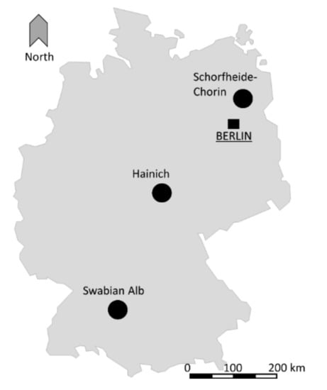
Figure 1.
Map of Germany highlighting the locations of the study areas.
2.2. Methods
2.2.1. Airborne Laser Scanning Data and Point Cloud Processing
Airborne laser scanning data were acquired in July, 2015 using a Q780 Riegl Sensor at an operating frequency of 400 kHz from a flight height of approximately 950 m above ground. This resulted in an average pulse density of 13 pls × m−2 with a mean pulse spacing of 29 cm, as observed for the areas of the 66 plots. As multiple returns were recorded per pulse, the average point density was 36.24 pts × m−2. The pre-processing was performed using LAStools [43]. This included the removal of isolated returns, retiling into 500 × 500 m tiles, classification of returns into ground and vegetation, and normalization of the elevation values to above ground level (AGL). Finally, the point clouds were clipped using the plot boundaries and the vegetation returns were exported as CSV files with the xyz-coordinates of each return. A visualization of the airborne LiDAR data of two exemplary plots from different perspectives is provided in Figure 2.
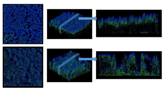
Figure 2.
Airborne light detection and ranging (LiDAR) point clouds of two example plots used in this study. Top: Plot AEW02; Bottom: Plot HEW48. Both point clouds are shown from top view, intermediate angle, and side view of exemplary cross-sections. Both plots are 1 ha in size (100 × 100 m). Further details on AEW02 and HEW48 are provided in Table 1. Colors indicate return intensity were not of importance in our analysis. We kept colors here only for better visualization.
Based on these CSV files, we calculated the box-dimension of each plot for the full 100 × 100 m with Mathematica software (Wolfram Research, Champaign, USA) and as described in the following. Based on all points in the point clouds, the algorithm determined the number of boxes of varying size that were needed to encapsulate all points. Starting with the minimum bounding cube (only one needed to enclose all points), the box sizes were consecutively reduced in steps that always cut the box edge length in half. Consequently, starting with 100 × 100 × 100 m, the next size was 50 × 50 × 50 m, 25 × 25 × 25 m, and so on, until the lower cut-off was reached. The lower cut-off was set as 50 cm as a highly conservative estimate of the point cloud resolution.
The box-dimension of a tree or forest can then be considered the slope of the fitted straight line through a graph of log(N) over log(1/r) [29,30,44]. Here, log() is the natural logarithm, N is the number of boxes (here: boxes) of size r (edge length in relation to the initial edge length used for the first box) needed to enclose all points of a tree or forest. Figure 3 provides a visual outline of the box-dimension calculation.
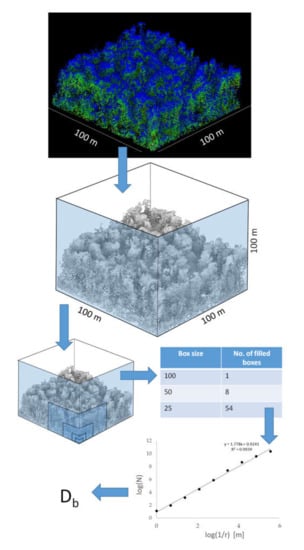
Figure 3.
Workflow for the determination of the box-dimension: exemplary plot HEW48 as original airborne LiDAR point cloud with return intensities shown as different colors (top; 366,486 points) and representation of points indicating the centers of the voxels of a 20 cm voxel model without coloring but with shading (middle; 267,379 points). Consecutive subset of boxes of decreasing size for an exemplary box only (lower left). Table contrasting box sizes with number of filled boxes (lower right). Bottom right: exemplary log-log plot with the slope representing the box-dimension (Db).
2.2.2. Terrestrial Laser Scanning and Point Cloud Processing
Terrestrial laser scans were conducted in Summer 2014 on all 66 plots, using a Faro Focus 3D 120 terrestrial laser scanner (Faro Technologies Inc., Lake Mary, USA). On a regular grid with 33 m spacing, we made nine scans per 1-ha plot; for details see [12,41]. All scans were set to scan with an angular resolution of 0.035° in horizontal and vertical directions. The total 594 single scans were then filtered for erroneous points using standard filters in Faro Scene (Faro Technologies Inc., Lake Mary, USA) and exported as xyz-files. Since the scans were used each on their own (single-scan approach), no merging procedure (co-registration) was necessary. Based on these xyz-files, we calculated the effective number of layers (ENL2D; [41]) as a measure of vertical structure, as well as the stand structural complexity index (SSCI; [12]), using the same algorithms as in the original work and Mathematica software. In short, ENL2D is a measure that first quantifies the number of vertical layers (1 m in thickness) that actually contain vegetation and secondly weighs the numbers based on the filling of the layers using the inverse Simpson index (more plant material in a layer = greater weight). The SSCI index uses vertical cross-sections through the point cloud to quantify the complexity of the surrounding forest scene based on the relationship between the perimeter of the polygon, connecting all points in a cross-section and the area enclosed by it. By using a 1280 cross-section for a 360° field of view in the azimuthal direction, a detailed description of the structure of the forest scene was provided. The interested reader is referred to [12,41] for more explanation and mathematical details on the two indices.
2.2.3. Additional Information on Plot Level
For each plot, we obtained information from the Biodiversity Exploratories database (http://www.bexis.uni-jena.de/PublicData/PublicData.aspx). This included stand age (see also Table 1; source: [45]; Dataset ID: 17486), management intensity as expressed by the silvicultural management index (abbreviated: SMI; [45]; Dataset ID: 17746), basal area ([46]; Dataset ID: 22907), structural complexity index by [23], and the coefficient of variation of the diameter of trees larger than 7 cm at breast height, both from Dataset ID 17687 [46,47].
Furthermore, we used the mean diurnal temperature range (DTR; see [18]; based on Dataset ID: 19007) as a measure of the “stability” of the forest microclimate.
2.3. Statistical Analysis
The open source software R (Vers.3.5, R Development Core Team) was used for all statistical analyses. The general relationship between the different variables and the box-dimension (Db) was described through the Spearman’s rank correlation coefficient (rho) as a non-parametric correlation measure, because a linear relationship between the variables could not be assumed. The significance of the correlation was assumed if the p-value of the correlation coefficient was <0.05, indicating the true rho to be not equal to 0.
We used Welch’s T-test to test for significant differences in structural complexity between coniferous and deciduous forest plots. The regression analysis between explanatory and response variables was conducted with generalized linear modeling techniques by applying generalized additive models to the data [48]. This method requires no predefinition of the relationship between response and explanatory variable, which allows the unbiased detection of trends in the data themselves. The exponential family distribution of the response variable was specified as normal along with an identity link function. The effective degrees of freedom were limited to a maximum of 3 to avoid over-fitting the data and allow the detection of general trends within the data [49]. The amount of smoothing was chosen automatically through generalized cross-validation [50].
3. Results
Despite some overlap, we found a significantly (p < 0.05) higher structural complexity (Db) for the investigated deciduous stands when compared to the coniferous stands (Figure 4).
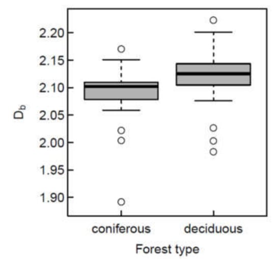
Figure 4.
Box-and-whisker plot of box-dimension for all 66 study sites, grouped as coniferous (n = 21) or deciduous (n = 45) forests. The differences in mean were significantly different from zero (p < 0.05).
We observed significant differences between the management types “age class forests”, pooling together all phases (thickets, polewoods, immature and mature stands), and “selection forests” (Figure 5a), considering all 66 plots. The structural complexity of unmanaged forests did not differ significantly from age class forests or selection forests.
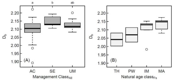
Figure 5.
Box-and-whisker plots of box-dimension from airborne laser scanning data for (A) all stands, and (B) only stands dominated by European beech (n = 42). In (A) Different lower-case letters indicate statistically significant differences between the groups AC: Age class forest, SE: Selection forest, UM: Unmanaged forest. In (B), we did not test for statistically significant differences among age classes due to two occasions of small sample sizes (n = 2 for thicket and polewood). TH: Thicket; PW: Polewood; IM: Immature; MA: Mature.
Considering only plots dominated by European beech (largest sample), we found an increasing trend in the box-dimension from thickets (mean: 2.04) over that of polewood (mean: 2.07) to immature (mean: 2.11) and mature forests (mean: 2.14) (Figure 5b). We did not test for significance when comparing the age classes due to the limited sample sizes of polewoods (n = 3) and thickets (n = 2).
The box-dimension (Db) derived from the airborne laser scanning data was significantly positively correlated with the stand structural complexity measures obtained from the ground-based measurements, namely the SSCI and SCI (see Figure 6A+B). It was also positively related to the coefficient of variation of diameters (Figure 6 C) and the effective number of layers (E), both measures describing forest structure. Furthermore, we found a positive relationship with stand age (F). Significant negative relationships were discovered for Db and management intensity (G) as well as the diurnal temperature range (H), the latter indicating an increased microclimatic stability (lower DTR) with increasing complexity. Basal area (Figure 6C) was not significantly related to the Db from airborne LiDAR.
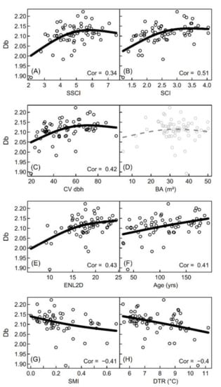
Figure 6.
Scatterplots of box-dimension from airborne LiDAR (Db) against measures of structural complexity (stand structural complexity index (SSCI) and structural complexity index (SCI); (A,B), against the coefficient of variation of diameters (CV_dbh; (C), basal area (BA; (D), the effective number of layers (ENL2D; (E), stand age (F), silvicultural management intensity (SMI; (G) and the diurnal temperature range (DTR; H). Spearman’s correlation coefficient (Cor) is presented for all p-values indicating that true rho is not equal to 0 (p < 0.05). Solid black lines indicate significance at the level of p < 0.05 of the smoothing terms in the generalized additive models. Grey dashed lines show non-significant parameter estimates of the smoothing term.
An overview of some numerical characteristics of the generalized additive models that have been visualized in Figure 6 are provided in Table 2.
Table 2.
Overview on several characteristics of the generalized additive models. Estimated degrees of freedom (EDF) = 1 if the model penalized the smooth term to a simple linear relationship; p.EDF = significance of smoothing; n= number of plots for which data was available. DevEx = Deviation explained.
4. Discussion
We first tested the performance of Db in differentiating between forest types (coniferous vs. deciduous). Db differed significantly for coniferous vs. deciduous stands even though we observed some overlap in the range of values. We argue that this is to be expected since, aside from forest type, the contrasted stands also differed in management regime, developmental phase, and geographical location. Furthermore, earlier research [12] already revealed that the coniferous stands pooled here have considerable differences in structural complexity depending on the main tree species (pine vs. spruce).
Secondly, the Db from airborne laser scanning (ALS) was evaluated for its performance in separating different management types. The unmanaged forests investigated here showed only intermediate structural complexity and did not differ from the age class stands forest or selection forests, which is a result of the short period since management ceased (~20 yrs). Furthermore, management ceased when the stands were in the optimum phase, which is naturally a phase of low structural complexity, particularly in the case of European beech [35]. The significant differences between age class forests and selection forests supports the hypothesis that the Db from ALS data is indeed capable of distinguishing structural patterns as a consequence of different management. While age class forests have a high variability in structural complexity if all age classes are considered together, they also tend to have the greatest complexity in the younger developmental phase, particularly in thickets [35]. The age class forests investigated here also showed great variability in structural complexity (Figure 6A) but may seem to contrast when it comes to the complexity of thickets. Instead of the highest values for thickets, we found a trend from low to high complexity for the successive developmental phases. We argue that this is due to the very limited number of shelter trees in our thickets. Usually, the remaining overstory trees add great complexity to thickets [35], but, in the case of the thickets investigated here, these trees have already been removed to a great extent. However, our findings must be interpreted with caution due to the small sample sizes of thickets (n = 2) and polewood (n = 3).
We further compared Db with various ground-based measures, including two measures of structural complexity, namely the stand structural complexity index (SSCI) and the structural complexity index (SCI). While SSCI is a holistic measure of structural complexity that is derived from terrestrial laser scanning (cf. [12]), SCI can be calculated from conventional inventory data. Both have proven useful in the past as surrogates of microclimatic stability (SSCI; [41]), classifiers of forest types (SCI: [23]; SSCI: [12] and [35]), or predictors of biodiversity, e.g., for ant species (SSCI:[51]) or tree species diversity (SSCI: [12]). Here, the birds-eye perspective of airborne laser scanning (ALS) yielded intermediate but significant correlations (R = 0.35 − 0.51) between Db and the two ground-based measures of structural complexity. It is hence not surprising that Db was also correlated with the coefficient of variation of the diameters at breast height (CV_dbh) as the latter is known to be strongly correlated to stand structural heterogeneity [46].
We showed that Db from airborne data, despite the possible effects of the occlusion of lower forest strata, was correlated with several ground-based measures that are related to stand structural complexity. The occlusion effects may have reduced the strength of the correlations but did not impede them. The observed correlation between Db and the effective number of layers (ENL2D), a measure of vertical structural evenness, supports this argument. Morsdorf et al. [52] also highlighted that ALS data can be used to discriminate forest strata even in multi-layered forests.
A relationship between structural complexity and basal area may be expected, since Db is dependent on stand density and material distribution in space [39]. Earlier studies found that basal area was related to Zenner and Hibbs’ SCI [53]. In addition, previous research showed that structural complexity measured using SSCI was dependent on stand density as well, even though space-filling was used instead of basal area as a measure of density [12]. However, space-filling considers the actual canopy space exploration and goes far beyond basal area (sensu [34,54]). Here, we argue that basal area was not related to Db since it is not a holistic measure of structural complexity. Basal area provides no information on the crown dimensions (those parts that are responsible for most of the complexity in a forest), but also trees below a certain threshold, usually 7 cm in diameter at breast height, are not included in its calculation based on standard inventory data. In contrast, in the point cloud, all trees are included and accounted for, regardless of their size. The absence of a significant correlation between Db and basal area may be a result of these fundamental discrepancies and leads to a rejection of hypothesis (ii).
We further hypothesized that Db would be related to the age of a stand. In our data, we found clear indications to support this hypothesis. With increasing stand age, structural complexity as measured by Db increased (Figure 6f). We argue that this is due to the increased structural complexity of the individual trees with age [30]. The effect was still evident when the forests were grouped according to the main tree species (data not shown), meaning that this relationship did not result from the fact that the deciduous stands in our study were on average older than the coniferous ones (see Table 1).
The observed negative relationship between the management intensity index (SMI) and Db confirmed the findings of Stiers et al. [35], who studied beech-dominated forests across a management gradient from intensively managed to unmanaged old-growth forests, clearly highlighting that the greatest complexity is to be found in old-growth stands (low SMI). ALS data has already shown a potential for addressing forest structure–management relationships in earlier studies. For example, Valbuena et al. [55] showed that the Gini coefficient derived from ALS data was useful to identify changes in forest structure due to management. Our findings on the relationship between Db and stand age and SMI are in line with these results and support our third hypothesis (iii).
Finally, hypothesis (iv) was also supported by our identification of a significant positive relationship between the microclimatic stability, here addressed using the diurnal temperature range, and the structural complexity (Db) of the stands. Earlier pilot studies already showed that structural complexity, when addressed from the ground using the TLS-based SSCI, was positively related to the microclimatic stability, reducing daily temperature fluctuations and the vapor pressure deficit [12].
Past research showed that a large number of forest metrics can be derived from ALS point clouds, including species identities [56,57], a plethora of structural measures [9,58], and even forest type classifications [10,59,60]. As a measure of structural complexity, Db was related to all measures tested in our study except basal area. The strength of the relationships may often only be weak or intermediate (R = 0.34 − 0.51), but we argue that this is to be expected if a holistic measure like Db, that uses basically all data in the point cloud to combine them into a single number, is related to the individual characteristics of a stand.
In earlier studies based on digitizers, measurements of Db were restricted to tree compartments, e.g., roots [61]. Terrestrial laser scanning (TLS) data expanded the application of fractal analysis to single trees or tree groups [13,29]. Here, we show that Db from ALS can be a useful descriptor enabling an assessment of forest structural complexity for 1-ha plots and theoretically much larger areas and even in difficult terrain. This supports the idea that applying fractal techniques at the stand level can yield new insights into forest structure [62].
5. Conclusions
Quantifying the structural complexity of forest stands is important to support a management for complexity, thereby strengthening ecosystem functioning and ecosystem services. We showed that the box-dimension (Db), as a measure of structural complexity that already showed potential in ground-based LiDAR applications, can also be derived from airborne laser scanning data. Using different ground-based measures for reference, we were able to show that ALS-derived Db has the potential to identify differences in forest type, management type, and developmental phase. Furthermore, it was sensitive to stand age, management intensity, and structural changes. Finally, it was related to an indicator of microclimatic stability in terms of temperature fluctuations in the stands.
Author Contributions
Conceptualization, D.S., P.A. and M.E.; Data curation, D.S. and P.M.; Formal analysis, D.S. and P.A.; Funding acquisition, D.S., P.M. and C.A.; Investigation, D.S. and P.M.; Methodology, D.S., P.A., M.E. and P.M.; Project administration, D.S.; Resources, D.S. and C.A.; Software, D.S. and S.W.; Supervision, D.S. and C.A.; Validation, D.S.; Visualization, D.S. and P.A.; Writing—original draft, D.S.; Writing—review & editing, D.S., P.A., M.E., P.M. and C.A. All authors have read and agreed to the published version of the manuscript.
Funding
The German Research Foundation (DFG) is acknowledged for funding this research through grant SE2383/5-1 provided to Dominik Seidel.
Acknowledgments
We thank the managers of the three Exploratories, Kirsten Reichel-Jung, Swen Renner, Katrin Hartwich, Sonja Gockel, Kerstin Wiesner, and Martin Gorke for their work in maintaining the plot and project infrastructure; Christiane Fischer and Simone Pfeiffer for giving support through the central office, Michael Owonibi for managing the central data base, and Markus Fischer, Eduard Linsenmair, Dominik Hessenmöller, Jens Nieschulze, Daniel Prati, Ingo Schöning, François Buscot, Ernst-Detlef Schulze, Wolfgang W. Weisser and the late Elisabeth Kalko for their role in setting up the Biodiversity Exploratories project. We thank Falk Hänsel, Stephan Wöllauer, Frank Suschke, Mathias Groß, Martin Fellendorf and Thomas Nauss for operation and maintenance of meteorological stations in the research plots.
Conflicts of Interest
The authors declare that there is no conflict of interest.
References
- Knoke, T.; Seifert, T. Integrating selected ecological effects of mixed European beech–Norway spruce stands in bioeconomic modelling. Ecol. Model. 2008, 210, 487–498. [Google Scholar] [CrossRef]
- Messier, C.C.; Puettmann, K.J.; Coates, K.D. Managing Forests as Complex Adaptive Systems: Building Resilience to the Challenge of Global Change; Routledge: London, UK, 2013. [Google Scholar]
- O’Hara, K.L.; Ramage, B.S. Silviculture in an uncertain world. Utilizing multi-aged management systems to integrate disturbance. Forestry 2013, 86, 401–410. [Google Scholar]
- Pommerening, A. Approaches to quantifying forest structures. Forestry 2002, 75, 305–324. [Google Scholar] [CrossRef]
- Puettmann, K.J. Silvicultural Challenges and Options in the Context of Global Change. “Simple” Fixes and Opportunities for New Management Approaches. J. For. 2011, 109, 321–331. [Google Scholar]
- Castel, T.; Guerra, F.; Caraglio, Y.; Houllier, F. Retrieval biomass of a large Venezuelan pine plantation using JERS-1 SAR data. Analysis of forest structure impact on radar signature. Remote. Sens. Environ. 2002, 79, 30–41. [Google Scholar] [CrossRef]
- Treuhaft, R.N.; Law, B.E.; Asner, G.P. Forest attributes from radar interferometric structure and its fusion with optical remote sensing. BioScience 2004, 54, 561–571. [Google Scholar] [CrossRef]
- Tebaldini, S.; Minh, D.H.T.; d’Alessandro, M.M.; Villard, L.; Le Toan, T.; Chave, J. The Status of Technologies to Measure Forest Biomass and Structural Properties. State of the Art in SAR Tomography of Tropical Forests. Surv. Geophys. 2019, 40, 1–23. [Google Scholar] [CrossRef]
- Kukunda, C.B.; Beckschäfer, P.; Magdon, P.; Schall, P.; Wirth, C.; Kleinn, C. Scale-guided mapping of forest stand structural heterogeneity from airborne LiDAR. Ecol. Indic. 2019, 102, 410–425. [Google Scholar] [CrossRef]
- Thers, H.; Bøcher, P.K.; Svenning, J.C. Using lidar to assess the development of structural diversity in forests undergoing passive rewilding in temperate Northern Europe. PeerJ 2019, 6, e6219. [Google Scholar] [CrossRef]
- Dubayah, R.; Blair, J.B.; Goetz, S.; Fatoyinbo, L.; Hansen, M.; Healey, S.; Hofton, M.; Hurtt, G.; Kellner, J.; Luthcke, S.; et al. The Global Ecosystem Dynamics Investigation: High-resolution laser ranging of the Earth’s forests and topography. Sci. Remote Sens. 2020, 1, 100002. [Google Scholar] [CrossRef]
- Ehbrecht, M.; Schall, P.; Ammer, C.; Seidel, D. Quantifying stand structural complexity and its relationship with forest management, tree species diversity and microclimate. Agri. For. Met. 2017, 242, 1–9. [Google Scholar] [CrossRef]
- Seidel, D.; Ehbrecht, M.; Annighöfer, P.; Ammer, C. From tree to stand-level structural complexity—which properties make a forest stand complex in structure? Agri. For. Met. 2019, 278, 107699. [Google Scholar] [CrossRef]
- Seidel, D.; Annighöfer, P.; Stiers, M.; Zemp, C.D.; Burkardt, K.; Ehbrecht, M.; Willim, K.; Kreft, H.; Hölscher, D.; Ammer, C. How a measure of structural complexity relates to architectural benefit-to-cost ratio, light availability and growth of trees. Ecol. Evol. 2019. [Google Scholar] [CrossRef] [PubMed]
- Filippelli, S.K.; Lefsky, M.A.; Rocca, M.E. Comparison and integration of lidar and photogrammetric point clouds for mapping pre-fire forest structure. Remote Sens. Environ. 2019, 224, 154–166. [Google Scholar] [CrossRef]
- Morin, D.; Planells, M.; Guyon, D.; Villard, L.; Mermoz, S.; Bouvet, A.; Thevenon, H.; Dejoux, J.F.; Le Toam, T.; Dedieu, G. Estimation and Mapping of Forest Structure Parameters from Open Access Satellite Images. Development of a Generic Method with a Study Case on Coniferous Plantation. Remote Sens. 2019, 11, 1275. [Google Scholar] [CrossRef]
- Alonzo, M.; Andersen, H.E.; Morton, D.C.; Cook, B.D. Quantifying boreal forest structure and composition using UAV structure from motion. Forests 2018, 9, 119. [Google Scholar] [CrossRef]
- Ehbrecht, M.; Schall, P.; Ammer, C.; Seidel, D. Effects of structural heterogeneity on the diurnal temperature range in temperate forest ecosystems. For. Ecol. Manag. 2019, 432, 860–867. [Google Scholar] [CrossRef]
- Hardiman, B.S.; Gough, C.M.; Halperin, A.; Hofmeister, K.L.; Nave, L.E.; Bohrer, G.; Curtis, P.S. Maintaining high rates of carbon storage in old forests: A mechanism linking canopy structure to forest function. For. Ecol. Manag. 2013, 298, 111–119. [Google Scholar] [CrossRef]
- Gough, C.M.; Atkins, J.W.; Fahey, R.T.; Hardiman, B.S. High rates of primary production in structurally complex forests. Ecology 2019. [Google Scholar] [CrossRef]
- Penone, C.; Allan, E.; Soliveres, S.; Felipe-Lucia, M.R.; Gossner, M.M.; Seibold, S.; Simons, N.K.; Schall, P.; van der Plas, F.; Manning, P.; et al. Specialisation and diversity of multiple trophic groups are promoted by different forest features. Ecol. Lett. 2019, 22, 170–180. [Google Scholar] [CrossRef]
- Aguirre, O.; Hui, G.; von Gadow, K.; Jiménez, J. An analysis of spatial forest structure using neighbourhood-based variables. For. Ecol. Manag. 2003, 183, 137–145. [Google Scholar] [CrossRef]
- Zenner, E.; Hibbs, D. A new method for modeling the heterogeneity of forest structure. For. Ecol. Manag. 2000, 129, 75–87. [Google Scholar] [CrossRef]
- Beckschäfer, P.; Mundhenk, P.; Kleinn, C.; Ji, Y.; Yu, D.; Harrison, R. Enhanced Structural Complexity Index: An Improved Index for Describing Forest Structural Complexity. Open J. For. 2013, 3, 23–29. [Google Scholar] [CrossRef]
- Clark, P.J.; Evans, F.C. Distance to nearest neighbor as a measure of spatial relationships in populations. Ecology 1954, 35, 445–453. [Google Scholar] [CrossRef]
- McElhinny, C.; Forest and woodland structure as an index of biodiversity. A Review. A Literature Review Commissioned by NSW National Parks and Wildlife Service. Available online: https://pdfs.semanticscholar.org/cb98/b45746fc5ae914b50eef0947fec87e5db1db.pdf (accessed on 10 January 2020).
- Martin-Ducup, O.; Robert, S.; Fournier, R.A. Response of sugar maple (Acer saccharum, Marsh.) tree crown structure to competition in pure versus mixed stands. For. Ecol. Manag. 2016, 374, 20–32. [Google Scholar]
- Malhi, Y.; Jackson, T.; Patrick Bentley, L.; Lau, A.; Shenkin, A.; Herold, M.; Calders, K.; Bartholomeus, H.; Disney, M.I. New perspectives on the ecology of tree structure and tree communities through terrestrial laser scanning. Interface Focus 2018, 8, 20170052. [Google Scholar] [CrossRef]
- Seidel, D. A holistic approach to determine tree structural complexity based on laser scanning data and fractal analysis. Ecol. Evol. 2018, 8, 128–134. [Google Scholar] [CrossRef]
- Seidel, D.; Ehbrecht, M.; Dorji, Y.; Jambay, J.; Ammer, C.; Annighöfer, P.J. Identifying architectural characteristics that determine tree structural complexity. Trees 2019, 33, 911–919. [Google Scholar] [CrossRef]
- Atkins, J.W.; Bohrer, G.; Fahey, R.T.; Hardiman, B.S.; Morin, T.; Stovall, A.; Zimmerman, N.; Gough, C.M. Quantifying vegetation and canopy structural complexity from terrestrial LiDAR data using the forestr R package. Methods. Ecol. Evol. 2018, 9, 2057–2066. [Google Scholar] [CrossRef]
- Willim, K.; Stiers, M.; Annighöfer, P.; Ehbrecht, M.; Kabal, M.; Ammer, C.; Seidel, D. Assessing understory complexity in beech-dominated forests (Fagus sylvatica L.) in Central Europe- from managed to primary forests. Sensors 2019, 19, 1684. [Google Scholar] [CrossRef]
- Newnham, G.J.; Armston, J.D.; Calders, K.; Disney, M.I.; Lovell, J.L.; Schaaf, C.B.; Strahler, A.H.; Danson, F.M. Terrestrial laser scanning for plot-scale forest measurement. Curr. For. Rep. 2015, 1, 239–251. [Google Scholar] [CrossRef]
- Juchheim, J.; Ammer, C.; Schall, P.; Seidel, D. Canopy space filling rather than conventional measures of structural heterogeneity explains productivity of beech stands. For. Ecol. Manag. 2017, 395, 19–26. [Google Scholar] [CrossRef]
- Stiers, M.; Willim, K.; Seidel, D.; Ehbrecht, M.; Kabal, M.; Ammer, C.; Annighöfer, P. A quantitative comparison of the structural complexity of managed, lately unmanaged and primary European beech (Fagus sylvatica L.) forests. For. Ecol. Manag. 2018, 430, 357–365. [Google Scholar] [CrossRef]
- Zellweger, F.; Braunisch, V.; Baltensweiler, A.; Bollmann, K. Remotely sensed forest structural complexity predicts multi species occurrence at the landscape scale. For. Ecol. Manag. 2013, 307, 303–312. [Google Scholar] [CrossRef]
- Valbuena, R.; Vauhkonen, J.; Packalen, P.; Pitkänen, J.; Maltamo, M. Comparison of airborne laser scanning methods for estimating forest structure indicators based on Lorenz curves. Isprs J. Photogramm. Remote Sens. 2014, 95, 23–33. [Google Scholar] [CrossRef]
- Jayathunga, S.; Owari, T.; Tsuyuki, S. Analysis of forest structural complexity using airborne LiDAR data and aerial photography in a mixed conifer–broadleaf forest in northern Japan. J. For. Res. 2018, 29, 479–493. [Google Scholar] [CrossRef]
- Mandelbrot, B.B. The Fractal Geometry of Nature. 1977. Available online: https://users.math.yale.edu/~bbm3/web_pdfs/encyclopediaBritannica.pdf (accessed on 15 January 2020).
- Da Silva, D.; Boudon, F.; Godin, C.; Puech, O.; Smith, C.; Sinoquet, H. A critical appraisal of the box counting method to assess the fractal dimension of tree crowns. In Proceedings of the Second International Symposium (ISVC 2006), Lake Tahoe, NV, USA, 6–8 November 2006. [Google Scholar]
- Ehbrecht, M.; Schall, P.; Juchheim, J.; Ammer, C.; Seidel, D. Effective number of layers: A new measure for quantifying three-dimensional stand structure based on sampling with terrestrial LiDAR. For. Ecol. Manag. 2016, 380, 212–223. [Google Scholar] [CrossRef]
- Fischer, M.; Bossdorf, O.; Gockel, S.; Hansel, F.; Hemp, A.; Hessenmoller, D.; Korte, G.; Nieschulze, J.; Pfeiffer, S.; Prati, D.; et al. Implementing large-scale and long-term functional biodiversity research. The Biodiversity Exploratories. Basic Appl. Ecol. 2010, 11, 473–485. [Google Scholar] [CrossRef]
- LAStools. Efficient LiDAR Processing Software (Version 181119, Academic). 2018. Available online: http://rapidlasso.com/LAStools (accessed on 18 January 2020).
- Sarkar, N.; Chaudhuri, B.B. An efficient differential box-counting approach to compute fractal dimension of image. IEEE T. Syst. Sci. Cyb. 1994, 24, 115–120. [Google Scholar] [CrossRef]
- Schall, P.; Ammer, C. How to quantify forest management intensity in Central European forests. Eur. J. For. Res. 2013, 132, 379–396. [Google Scholar] [CrossRef]
- Schall, P.; Schulze, E.D.; Fischer, M.; Ayasse, M.; Ammer, C. Relations between forest management, stand structure and productivity across different types of Central European forests. Basic App. Ecol. 2018, 32, 39–52. [Google Scholar] [CrossRef]
- Schall, P.; Ammer, C. Forest EP stand Structure and Composition. v1.4.5. Biodiversity Exploratories Information System. Dataset. Available online: https.//www.bexis.uni-jena.de/PublicData/PublicData.aspx?DatasetId=17687 (accessed on 15 December 2019).
- Wood, S.N. Generalized Additive Models: An Introduction with R, 2nd ed.; CRC Press: Portland, OR, USA, 2017. [Google Scholar]
- Otto, S.A.; Diekmann, R.; Flinkman, J.; Kornilovs, G.; Möllmann, C. Habitat heterogeneity determines climate impact on zooplankton community structure and dynamics. PLoS ONE 2014, 9, e90875. [Google Scholar] [CrossRef] [PubMed]
- Ciannelli, L.; Chan, K.-S.; Chan, K.-S.; Bailey, K.M.; Stenseth, N.C. Nonadditive effects of the environment on the survival of a large marine fish population. Ecology 2004, 85, 3418–3427. [Google Scholar] [CrossRef]
- Grevé, M.E.; Hager, J.; Weisser, W.W.; Schall, P.; Gossner, M.M.; Feldhaar, H. Effect of forest management on temperate ant communities. Ecosphere 2018, 9, e02303. [Google Scholar] [CrossRef]
- Morsdorf, F.; Mårell, A.; Koetz, B.; Cassagne, N.; Pimont, F.; Rigolot, E.; Allgöwer, B. Discrimination of vegetation strata in a multi-layered Mediterranean forest ecosystem using height and intensity information derived from airborne laser scanning. Remote Sens. Environ. 2010, 114, 1403–1415. [Google Scholar] [CrossRef]
- Pasher, J.; King, D.J. Development of a forest structural complexity index based on multispectral airborne remote sensing and topographic data. Can. J. For. Res. 2010, 41, 44–58. [Google Scholar] [CrossRef]
- Seidel, D.; Leuschner, C.; Scherber, C.; Beyer, F.; Wommelsdorf, T.; Cashman, M.J.; Fehrmann, L. The relationship between tree species richness, canopy space exploration and productivity in a temperate broad-leaf mixed forest. For. Ecol. Manag. 2013, 310, 366–374. [Google Scholar] [CrossRef]
- Valbuena, R.; Eerikäinen, K.; Packalen, P.; Maltamo, M. Gini coefficient predictions from airborne lidar remote sensing display the effect of management intensity on forest structure. Ecol. Indic. 2016, 60, 574–585. [Google Scholar] [CrossRef]
- Kim, S.; McGaughey, R.J.; Andersen, H.E.; Schreuder, G. Tree species differentiation using intensity data derived from leaf-on and leaf-off airborne laser scanner data. Remote Sens. Environ. 2009, 113, 1575–1586. [Google Scholar] [CrossRef]
- Ørka, H.O.; Næsset, E.; Bollandsås, O.M. Classifying species of individual trees by intensity and structure features derived from airborne laser scanner data. Remote Sens. Environ. 2009, 113, 1163–1174. [Google Scholar] [CrossRef]
- Hermosilla, T.; Ruiz, L.A.; Kazakova, A.N.; Coops, N.C.; Moskal, L.M. Estimation of forest structure and canopy fuel parameters from small-footprint full-waveform LiDAR data. International journal of wildland fire. Int. J. Wildland Fire 2014, 23, 224–233. [Google Scholar] [CrossRef]
- Adnan, S.; Maltamo, M.; Coomes, D.A.; García-Abril, A.; Malhi, Y.; Manzanera, J.A.; Butt, N.; Morecroft, M.; Valbuena, R. A simple approach to forest structure classification using airborne laser scanning that can be adopted across bioregions. For. Ecol. Manag. 2019, 433, 111–121. [Google Scholar] [CrossRef]
- Almeida, D.R.A.; Stark, S.C.; Chazdon, R.; Nelson, B.W.; Cesar, R.G.; Meli, P.; Gorgens, E.B.; Duarte, M.M.; Valbuena, R.; Moreno, V.S.; et al. The effectiveness of lidar remote sensing for monitoring forest cover attributes and landscape restoration. For. Ecol. Manag. 2019, 438, 34–43. [Google Scholar] [CrossRef]
- Bouda, M.; Caplan, J.S.; Saiers, J.E. Box-counting dimension revisited: Presenting an efficient method of minimizing quantization error and an assessment of the self-similarity of structural root systems. Front. Plant Sci. 2016, 7, 149. [Google Scholar] [CrossRef]
- Drake, J.B.; Weishampel, J.F. Multifractal analysis of canopy height measures in a longleaf pine savanna. For. Ecol. Manag. 2000, 128, 121–127. [Google Scholar] [CrossRef]


© 2020 by the authors. Licensee MDPI, Basel, Switzerland. This article is an open access article distributed under the terms and conditions of the Creative Commons Attribution (CC BY) license (http://creativecommons.org/licenses/by/4.0/).