Self-Supervised Representation Learning for Remote Sensing Image Change Detection Based on Temporal Prediction

Abstract

Traditional change detection (CD) methods operate in the simple image domain or hand-crafted features, which has less robustness to the inconsistencies (e.g., brightness and noise distribution, etc.) between bitemporal satellite images. Recently, deep learning techniques have reported compelling performance on robust feature learning. However, generating accurate semantic supervision that reveals real change information in satellite images still remains challenging, especially for manual annotation. To solve this problem, we propose a novel self-supervised representation learning method based on temporal prediction for remote sensing image CD. The main idea of our algorithm is to transform two satellite images into more consistent feature representations through a self-supervised mechanism without semantic supervision and any additional computations. Based on the transformed feature representations, a better difference image (DI) can be obtained, which reduces the propagated error of DI on the final detection result. In the self-supervised mechanism, the network is asked to identify different sample patches between two temporal images, namely, temporal prediction. By designing the network for the temporal prediction task to imitate the discriminator of generative adversarial networks, the distribution-aware feature representations are automatically captured and the result with powerful robustness can be acquired. Experimental results on real remote sensing data sets show the effectiveness and superiority of our method, improving the detection precision up to 0.94–35.49%.

1. Introduction

Remote sensing image change detection (CD) is the process of identifying differences in the geographical area of interest over time. It plays a vital role in environmental monitoring applications, e.g., disaster evaluation and prevention, urban growth tracking and deforestation analysis, and land use and land cover monitoring [1,2,3]. With the advance of sensor technology, the increasing availability of remotely sensed images makes it possible to timely monitor the surface of the earth. However, owing to the imaging inconsistencies on many respects (e.g., brightness, contrast and noise distribution, etc.), automatic and efficient CD techniques are very challenging for bitemporal remotely sensed images [4]. The complex background caused by the complicated topography also impairs precise detection [5].

Over the past few decades, various CD methods have been proposed to effectively obtain the variations of earth surface [6,7,8]. In terms of whether they require manual labels, most of them can be grouped into supervised and unsupervised methods. For unsupervised CD ones, there are two major stages: (1) generating a difference image (DI) from co-registered image pairs; (2) analyzing the DI to obtain the final change map [9,10].

The DI is usually obtained by comparing bitemporal images in a pixelwise fashion. The significantly different pixels are considered as changed parts, and otherwise as unchanged ones. Image arithmetical operation is the common approach including image subtraction, image ratioing, and image regression, etc. [9,11,12]. The most common methods are image ratioing, which can transform the multiplicative noises into additive ones and thus is more robust to calibration errors [13]. Additionally, the change vector analysis (CVA) method is widely used in multispectral images. It obtains magnitude and direction of changed information by subtraction of corresponding spectral bands [14]. Having the obtained DI, DI analysis algorithms are needed to divide difference information into changed and unchanged categories. Many automatic methods are developed in the second stage [15]. The common methods include clustering methods, thresholding methods, image transformation methods, etc. [16,17]. In this stage, although a variety of methods are developed, they suffer from the propagated error of the quality of DIs.

How to achieve a high quality of DI that highlights the changed information and suppresses unchanged information is of vital importance in this unsupervised pipeline. Most existing methods operate in simple image domain or hand-crafted features to generate a DI. This leads to the generated DIs with poor representative capacity to complex change scenarios. In particular, they are not robust enough to noises and other irrelevant variations caused by sun angle, shadow and topography impact, etc. [9]. Further, the DI with poor quality causes that changed and unchanged information is severely overlapped, and cannot be divided by DI analysis accurately and readily.

High-level feature representations are promising to improve the performance of DI generation and enhance the robustness of detection results. At present, deep learning is considered as the most powerful feature learning method. It can extract abstract and hierarchical features from raw data. The learned features have been shown to be far superior to hand-crafted features in performance [18]. In computer vision, a large number of breakthrough works is based on deep learning technology [19,20,21]. However, different from unsupervised methodology, most deep network models depend on semantic annotations to learn robust feature representations, namely, supervised. In the remote sensing community, it is difficult to collect accurate semantic annotations, because of the high cost and amount of effort and time as well as the expert knowledge that are needed. Therefore, there is an urgent need to develop unsupervised CD methods for remote sensing images. Recently, generative adversarial networks (GAN) have gained in popularity, being adopted for many tasks such as object tracking [22], image generation [23,24], and semantic segmentation [25]. As a successful unsupervised learning model, GAN consists of two networks, i.e., a generator and a discriminator. The two networks alternately perform training by optimizing an adversarial objective. Motivated by the unsupervised working mechanism of GAN, we proposed a self-supervised methodology for learning high-level representations from a pair of remote sensing images, in which the difficulties of the acquisition of semantic supervision are successfully sidestepped and the temporal signal of CD data is explored as a free and plentiful supervision. In fact, self-supervised learning algorithms, as a branch of unsupervised learning algorithms, have been very early put forward to learn general feature representations from unlabeled image and video data without using any manual labels [26]. Instead, the structure information of data are usually excavated as supervised signal to learn useful representations, which are very beneficial for subsequent objective task such as the methods for video track and image restoration [27,28,29]. However, there are few self-supervised methods in the field of CD.

In our method, the self-supervised strategy is driven by temporal prediction to learn the visual feature representations, which are more consistent and discriminative to directly compare the difference, leading to a better DI where changed areas are significantly enhanced and unchanged ones are suppressed. This also relieves the difficulty of DI analysis for the final change map. Similar to most self-supervised methods, our self-supervised idea takes into full account the characteristics of data in remote sensing image CD itself. Unlike the common classification task, where the input to a classifier is assumed to be a single image [20], in a CD task, the input is often considered to be a pair of images. In terms of the type of sensors that acquire the two images, CD methods can be summarized into two categories based on homogeneous and heterogeneous images ( Heterogeneous image pairs are captured by different sensors, having distinct modality in the same ground object [30]. Usually, it is not feasible to directly compare in the original low-dimension space.), respectively. In this paper, we consider detecting changes from the two images that are captured by the same type of sensors, i.e., homogeneous images. Homogeneous sensors capture the same statistical properties of the same ground objects, in which the same intensity distribution can be assumed to be linearly correlated between image pairs [30]. Based on this observation, we design the pretext task that asks a network to differentiate a sample patch between the two satellite images. Due to enough similarity, the same distribution will be hardly identified between image pairs by the network. We define this case as “Cannot differentiate”, which actually captures the linear correlation of the same distribution between homogeneous image pairs and thus builds a joint feature space of distribution. In the feature space, the same ground objects between raw image pairs are represented to be more consistent, while the irrelevant variations are eliminated. Thereby, general feature learning is implemented based on the temporal prediction task without any semantic prior knowledge.

The key principle of our self-supervised method roots in GAN, i.e., adequate similar samples can hardly be differentiated between their corresponding data source. By analogy, with GAN [31], as it cannot differentiate, similar samples from raw image pairs will be regulated into the same probability $\frac{1}{2}$ by an optimal discriminator of a GAN. Such discriminative mechanism can be viewed as analogous to human in decision which temporal image a sample patch is from. Cannot differentiate is regarded as the same class with the probability $\frac{1}{2}$ of random guessing. With this, the proposed method can automatically capture the distribution of similar samples from two images and narrow their distance. In addition, the intensity distribution between image pairs can be grouped into two cases, i.e, common distribution and non-common distribution shown in Figure 1. Cannot differentiate corresponds to common distribution (similar samples) between two images. Naturally, the optimal discriminator will be able to separate the unique distribution (non-common distribution) that only exists in one of two images and thus enlarge their distance. We define this case as “Can differentiate”. Therefore, in the built discriminative learning feature space, the underlying distribution regularities between image pairs are automatically captured via the similarity metric of Cannot differentiate and Can differentiate, in which the irrelevant variations caused by sun angle, shadow, and topography impact are effectively suppressed and image pairs are represented more consistently. Then, the transformed consistent features are used to directly compare and generate a DI. Because difference measurement is applied to the new feature space rather than raw image domain or hand-crafted features, they effectively boost the performance of DI generation. Finally, a simple clustering algorithm is used to cluster the DI to obtain the final change map.

Moreover, by analogy to the ordinary GAN architecture, in our learning process, the similar distribution between two images actually serves as the real and fake samples. This situation can be viewed as the generator has already generated the fake samples that are similar enough to the real ones. Therefore, there is no need to train a generator that can be assumed to be frozen. With this, our method fully excavates and leverages the similarity, or said linear correlation, of the same distribution between image pairs to learn useful representations. In terms of comparing to GAN, our method avoids the calculations related to a generator and the efforts towards the training difficulties of the complete GAN. In short, based on the working mechanism of GAN, we design the self-supervised strategy that learns more robust and discriminative feature representations in a fully unsupervised manner.

Furthermore, different from existing methods that learn robust features based on changed and unchanged pairs, our learned feature representations are distribution-aware. In terms of this, our method is similar to image segmentation that merges homogeneous regions and divides the heterogeneous regions in an image such as superpixel-based [32,33], watershed-based [34,35], and level set segmentation methods [36,37]. However, these methods aim to label an image and are usually used to segment a DI for CD as aforementioned clustering and thresholding methods. When a segmentation method is separately applied to two raw images, the two segmented maps are compared and generate the change map, which is called “postclassification comparison” discussed in Section 2. In contrast, the goal of our method is not labeling two images, instead it is to focus on learning their discriminative and clean representations. Therefore, our method can be cast as denoising. Nevertheless, denoising methods are often applied to two images independently as preprocessing to detect changes, which cannot improve the consistency between two images. Our method can not only reduce the noise but also improve the consistency by bridging their representation space, which is significant to compare the difference occurred between two images.

The contributions of this work are summarized as follows.

• To the best of our knowledge, this is the first work to built a discriminative mapping framework to extract discriminative feature representations for direct comparison and detecting the changes. In the learning process, the temporal signal of data is used as a free supervised signal, so that our framework precludes complex additional works for the need of prior changed and unchanged knowledge, and does not introduce additional calculation cost.
• The proposed framework leverages the characteristic of homogeneous image pairs to learn their general feature representations. As the leaned representations are more consistent and discriminative for comparing the difference, the corruption of the irrelevant variations, such as speckle noises, brightness, and topography impact occurred between two images, has been avoided at a significant margin, which enables our method to be robust for generating the final change map.

This paper is organized into five sections. Section 2 discusses the related works of this study. Section 3 describes the main process of the proposed approach in detail. Experimental results on real remote sensing data sets are presented in Section 4, demonstrating the feasibility and superiority of the proposed approach. Section 5 draws a conclusion for our work.

2. Related Work

A. Traditional Change Detection Methods.

Traditional CD methods for remote sensing images can be summarized into two major categories: (1) postclassification comparison, which independently classifies two images and compares their classified maps. Changed areas are considered being the pixels that belong to different categories in the two maps. This method [38] can avoid radiation normalization of bitemporal images captured from different sensors and environmental conditions. However, it requires high classification accuracy for each of two images, and easily suffers from cumulative classification errors. (2) Postcomparison analysis, which includes the aforementioned two steps: generation of DI and analysis of DI. Most existing CD methods in remote sensing images follow this workflow because they can obtain changes without supervision [9,10].

In the generation of DI, in addition to being a widely used image arithmetical operation, image fusion methods have been developed to overcome the disadvantages of a single operator and deal with nonlinearity of changes [17]. Gong et al. [17] proposed a wavelet fusion method that integrates mean-ratio image and log-ratio image to suppress noises and keep more details of the changes. Gong et al. [13] also used grayscale and texture information to construct difference images (DIs), in which log-ratio image offers gray intensity changes and Gabor filter is used to obtain texture difference information. Analyzing DI can be viewed as an image segmentation task [39]. The main solutions are clustering methods and thresholding methods. Generally, a thresholding method separates changes from unchanges by finding an optimal threshold such as Kittler and Illingworth minimum-error thresholding algorithm [7], Otsu’s algorithm [16]. Such methods rely on the statistical properties of data, while the statistical distributions of changes and unchanges can not be modeled accurately [40]. The most common clustering method is fuzzy c-means (FCM) method [39], which assigns similar memberships to data into the same class and maintains the minimum inter-classes distance by optimizing an objective function. In some cases, the FCM algorithm has the advantages of retaining more image information than hard clustering such as k-means clustering algorithm [15]. However, standard FCM algorithm is sensitive to noises because it ignores the spatial context information [17]. Accordingly, many advanced context information-based methods are introduced [15,17,41]. Turgay et al. [42] presented a robust fuzzy local information C-means clustering algorithm (FLICM) for image segmentation, in which a fuzzy local similarity measure is introduced to resist noises and preserve image details. Gong et al. [43] combined Markov random field with FCM clustering to classify changed and unchanged areas in SAR images. In addition, image transformation-based methods are also introduced to reduce noise impact. The most common image transformation method is principal component analysis (PCA) [15]. It extracts feature vectors from nonoverlapping blocks of a DI obtained by image arithmetical operation. Then, the K-means method is applied to classify feature vectors into changed and unchanged classes. Furthermore, graph cut [44], artificial immune system [45], and saliency extraction [46] are also applied to DIs and obtain change maps.

As described above, traditional CD methods are briefly introduced. They usually operate in simple image domain or hand-crafted features, leading to restrictive robustness to noise. In this paper, we propose a deep feature representation learning method that extracts discriminative features from image pairs and compares them in high-level feature space for the changes. As a result, a better DI is achieved, which reduces the propagated error from DI and improves detection robustness.

B. Deep Learning-Based Change Detection Methods.

The recent developments indicate that deep learning techniques have achieved striking performance contributed by robust and abstract feature extraction [21,47]. Following them, deep learning-based CD methods have been widely explored [48]. Due to the lack of annotated samples for training a classifier, much attention has been paid to unsupervised deep learning-based CD methods. According to the difference of training mode, we further group them into semisupervised methods, unsupervised methods, and GAN-based methods.

Semisupervised methods. This kind of method models the CD problem as a classification task that learns robust features driven by a suitable training set. It usually includes four phases for detecting changes. First, an initial change map is obtained as pseudo-labels. Then, labeled training samples are constructed according to the pseudo-labels. Next, labeled training samples are used to train a classifier based on deep models for learning features and identifying changed pixels from unchanged ones. Finally, raw image data is fed into the trained networks to obtain the final change map [38,49]. For instance, in [38], the stack deep belief networks are built to learn changed and unchanged concept, and the change map is directly generated by the trained networks. Gong et al. [50] proposed a novel CD method by integrating superpixel-based feature extraction and difference representation learning with deep architecture for high-resolution multispectral images. In [51], the authors explored how a pair of patches being merged is better to extract feature descriptor for SAR image CD and proposed Siamese sample convolutional neural networks (SSCNN) to achieve feature extraction and change discrimination. Wang et al. [49] presented a general end-to-end 2-D convolutional neural network framework (GETNET) for hyperspectral images CD, in which the discriminative features are extracted from mixed affinity matrices that integrate subpixel information. In [52], the log-ratio operator and a hierarchical FCM algorithm are used to obtain an initial change map, and then training sets are selected from the initial change map. The less-noise representations and final feature classification are achieved by a convolutional-wavelet neural network (CWNN) driven by the training sets. In order to learn discriminative features for a specific classifier, the above-mentioned frameworks incorporate traditional methods or hand-crafted features to construct labeled sample sets, which show more robustness and superiority than traditional methods. However, they obtain available labels of training sets by deriving from an initial change map that is not entirely correct. In these methods, the potential of the network learning and predicting is not fully released.

Unsupervised methods. To further overcome the dependency on labeled data, several approaches are developed with no supervision [50,51]. Similar to our work, these methods aim to learn clearer and more consistent feature representations and achieve a DI. Traditional clustering or thresholding methods are adopted to segment the DI and obtain changed and unchanged areas. In such methods, there are not explicit labels to guide the optimization of the networks instead of a well-designed loss function based on pixel-wise difference. Liu et al. [30] designed a symmetric convolutional coupling network (SCCN) for heterogeneous image CD, where the network parameters are updated by applying a coupling function. Zhao et al. [18] described an approximately symmetric deep neural network to transform raw image pairs into more consistent feature representations, considering both changed and unchanged pixels to update parameters by introducing cluster information. Zhan et al. [53] proposed an iterative feature mapping network framework for obtaining multiple changes between heterogeneous pairs, in which stacked denoising autoencoder is first applied to extract features and hierarchical tree-based clustering analysis is used to achieve multiple changes. Their methods focus on shrinking the distance between unchanged pixels and enlarging the changed ones to build a consistent feature space, where a DI is generated. In these methods, changed and unchanged prior knowledge is needed to guide the training of the network, and they suffer from additional computation and manual parameter. Different from them, we transform features into a shared feature space by making the difference of common distribution be as small as possible, and the non-common distribution as large as possible. This avoids the need of prior knowledge and leads to a simpler and more effective method for capturing consistent feature representations for generating a DI in homogeneous images.

GAN-Based methods. Recently, adversarial learning has received much attention in deep learning because of its ability to discover and generate rich, hierarchical features. In [54], Gong et al. used GAN to model a better DI distribution from training data between bitemporal images, and FLICM is applied to the DI for obtaining the change map. Niu et al. [55] combined a conditional generative adversarial network (cGAN) and an approximation network to translate optical image with SAR image property, from which direct comparison for the change map becomes feasible. In [56], the authors proposed a generative discriminatory classified network (GDCN) for multispectral image CD, where the discriminator gains the ability of classification for change and unchange by learning from labeled data, unlabeled data, and fake data generated by GAN. These methods incorporate the usual architecture of GAN to learn representations for boosting CD performance, but they also introduce their own set of challenges such as training difficulty caused by a mass of learnable parameters and an adversarial optimization objective. In addition, simple existing methods are adopted to generate training sets and then learn semantic concept for change and unchange. For acquiring more reliable training sets, Hou et al. [57] collected a large-scale data set with manually annotated ground truths and proposed detecting changes from W-Net to CDGAN in high-resolution remote sensing images. The W-Net is an end-to-end dual-branch architecture (W-Net) that performs the feature expression of two bitemporal images and yields a change map directly. The W-Net is then used as a generator of a GAN framework for improving the final classification performance, forming a CDGAN architecture. This method is fully supervised, and thus is less appealing because of the difficulty of annotation by humans. Our proposed framework fully considers the working mechanism of GAN and characteristics of CD problem to automatically learn robust feature representations, without introducing additional model components that also need training. Then, our method extends a discriminator of a GAN to feature learning for remote sensing image CD, which is has lesser dependency and does not suffer from training difficulty of the complete GAN.

C. Other Self-Supervised Learning Methods.

As our method is not based on an exact GAN architecture instead of its working mechanism with a discriminator, it falls into the paradigm of self-supervised learning. Self-supervised learning implies there is no need for human annotation but supervisory learning techniques can still work [58]. Here, a pretext task is used to substitute human annotation so the algorithm is without supervision in a sense. For example, Wang et al. [59] used images and their transformed copies to produce sample sets with pseudo-labels for remote sensing image registration. The authors of [27] leveraged the temporal coherence of tracked objects between adjacent frames for video track. Fernando et al. [28] designed the networks to recognize the odd video-clip from sampled subsequences for video representation learning. Doersch et al. [29] trained the networks to predict the relative spatial location of patches in an image to capture the visual similarity across images, which can accomplish visual discovery of objects. These self-supervised learning methods show the structure of the data is utilized to provide supervisory signals such as aforementioned temporal coherence, odd video clip of video data and relative spatial location of patches in an image. By contrast, we sample patches centered on pixels from each of bitemporal images and ask a model to learn to predict which temporal image the patches come from. The free and plentiful temporal signal is explored as a supervisory signal to extract useful feature representations for CD, avoiding semantic annotations that are difficult to obtain. Concretely, by analogy with GAN, training such pretext task can transform raw image information into a specific feature space, where the irrelevant variations are suppressed and their feature representations become more consistent and abstract. More consistent and abstract representations are beneficial to significantly highlight changed pixels and suppress unchanged pixels for subsequent DI generation and analysis. For the benefit of retrieval, the investigation of comparison is concisely summarized in

Table 1. Summary of contemporary CD methods.

Method	Category	Pros and Cons	Examples
Traditional CD methods	Postclassification comparison	Can avoid radiation normalization from different sensors, but easily suffer from cumulative classification errors	[60,61]
	postcomparison analysis	The mainstream with excellent performance, but rely heavily on the quality of a DI	[13,16,17,39]
Deep learning CD methods	Semisupervised methods	The current mainstream, be superior to traditional methods, but rely heavily on the quality of pseudo-labels	[38,49,50,52]
	Unsupervised methods	Introduce many additional manual parameter with complex optimizing process, often perform better on heterogeneous images than on homogeneous ones	[18,19,30]
	GAN-Based methods	Aim to improve the detection performance by the adversarial process, but also introduce challenges of GAN itself, e.g., training difficulty	[54,55,56]
	Self-Supervised methods	Independent of semantic supervision, easily obtain supervised signal, robust to noise, but rely on the quality of extracted features	The proposed method

. In the next section, we will describe our self-supervised representation learning methodology in detail.

3. Methodology

Given the two coregistered intensity images: $I_1=\left\{I_1(i,j)\right|1\le i\le W,1\le j\le H\}$ and $I_2=\left\{I_2(i,j)\right|1\le i\le W,1\le j\le H\}$, acquired over the same geographical area at different times, $W\times H$ is the size of images. The proposed self-supervised representation learning method can obtain their feature maps with powerful representation abilities, so that achieve a change map $B^{W\times H}$: $B(i,j)\in \{0,1\}$, where 1 indicates the pixel coordinate $(i,j)$ has occurred change, 0 indicates unchanged one. The work flow of the proposed method is depicted in Figure 2. In this section, we will first present the overview of the self-supervised mechanism and illustrate the proposed network architecture in detail. Then, the establishment and training of the instance based on deep neural networks (termed as discriminative adversarial deep neural networks (DADNN)) are presented, and the detailed mapping results are discussed. Finally, we deal with mapping-based binary segmentation and obtain the final change map.

3.1. Overview of Self-Supervised Mechanism for Learning Useful Representations

Our aim is to learn high-level and discriminative feature representations for CD with the proposed self-supervised mechanism. It is driven by the pretext task, i.e., predicting which temporal image ($I_1$ or $I_2$) the patches centered on pixels come from. Then, the task is designed to imitate a discriminator of a GAN. As a result, the linear correlation of the same intensity distribution between image pairs is captured and the discriminative representations of the image pairs are obtained. To this end, let us briefly review GAN, as originally introduced by Goodfellow et al. in 2014 [31]. It consists of two networks: one is the generator G that aims to learn a generator distribution $p_g$ similar to the real data distribution $p_{data}$ over sample x, and the other is the discriminator D that is trained to distinguish between two different distributions, or said, the source of samples, i.e., generated by G or the real data. During training, an alternate strategy is adopted to simultaneously optimize the two networks by the following minimax objective function,

$$\begin{array}{cc}\hfill \underset{G}{min}\underset{D}{max}V(D,G)=& E_{x\sim p_{data}\left(x\right)}[logD\left(x\right)]+\hfill \\ \hfill & E_{z\sim p_z\left(z\right)}[log(1-D(G\left(z\right)\left)\right)]\hfill \end{array}$$

(1)

where $p_z\left(z\right)$ is a noise variable that will be transformed by G into the samples $G\left(z\right)$. When G generates the samples whose distribution, $p_g$, is similar enough to the real sample distribution $p_{data}$, i.e., $p_g=p_{data}$, there exists a unique solution $D_G^{*}\left(x\right)=\frac{1}{2}$ everywhere. That means D and G have enough capacity and D is unable to differentiate between the real data distribution $p_{data}$ and the generator’s distribution $p_g$.

The key idea to unsupervised adversarial learning by GAN is that the discriminator is used to differentiate the source of samples until cannot differentiate, so that the generator can generate similar image distribution to the real training images [31,55].

In the CD task, two remote sensing images being captured by the same sensor, the same ground object has the similar statistical property. In feature space, their similar visual representations should be hardly differentiated between their corresponding data source, i.e, images $I_1$ and $I_2$. Following a discriminator of a GAN, the network trained for temporal prediction will output two possible identification results. According to the characteristic of distribution between image pairs, the main one is Cannot differentiate, the other is Can differentiate. The latter is where our discriminative method differs from an optimal discriminator of a GAN, as it only includes the Cannot differentiate that corresponds to common distribution. As shown in Figure 1, a patch sampled from one of two images either belongs to common distribution or does not, i.e., belongs to non-common one. Depending on which distribution the sample comes from, its recognition result is obtained. This can be viewed as a feature transformation/mapping operator, which bridges the representations between image pairs and enables them to be consistently represented by Cannot differentiate and Can differentiate. Thereby, distribution-aware feature representations of two input images are learned by the network trained for temporal prediction.

Here, we analyze the specific process of feature mapping for each case of distributions, while imitating a discriminator of a GAN. Specifically, we sample neighborhood of each pixel from each of two images as a sample patch x. As shown in Figure 3, the samples $x_1^{land}$ and $x_2^{land}$ come from the land area in image $I_1$ and image $I_2$, respectively. They are very similar and can hardly be discriminated. In the water areas, $x_1^{water}$ and $x_2^{water}$ are in the same situation. As mentioned above, this is in line with the optimizing objective of GAN to be alternately trained. The fake samples generated by the G are similar enough to the real samples, and the optimal $D^{*}$ cannot differentiate between the real and generated samples, i.e., $D^{*}\left(x\right)=\frac{1}{2}$. Taking $x_1^{land}$ and $x_2^{land}$ for example, as long as we treat one of $x_1^{land}$ and $x_2^{land}$ as the sample generated by the G, the other one acts as the real sample, we can obtain $D^{*}\left(x_1^{land}\right)=\frac{1}{2}$ and $D^{*}\left(x_2^{land}\right)=\frac{1}{2}$ by training the D. Such results have rigorous proof in the ordinary GAN. Intuitively, we cannot differentiate between $x_1^{land}$ and $x_2^{land}$ because they are very similar, so the discriminative probability is equal to random guessing, each of which is half chance. By this, the probability of similar samples will be pulled to the same direction, i.e., close to the probability $\frac{1}{2}$, and simultaneously the distance between similar samples from image pairs is shrank continually as the D is trained. Besides, for the non-common distribution, its unique reality has not be shared in two images. That means, the optimal $D^{*}$ can easily distinguish samples from image $I_1$ rather than $I_2$. Their probability given by the optimal $D^{*}$ will close to their corresponding labels, i.e., 0 or 1. Therefore, the same intensity distributions between image pairs are automatically clustered and expressed to be more consistent by the output probabilities with Can differentiate and Cannot differentiate, where noises are greatly reduced. With this, the free supervision is enabled to be feasible for learning the high-level feature representations from raw image pairs.

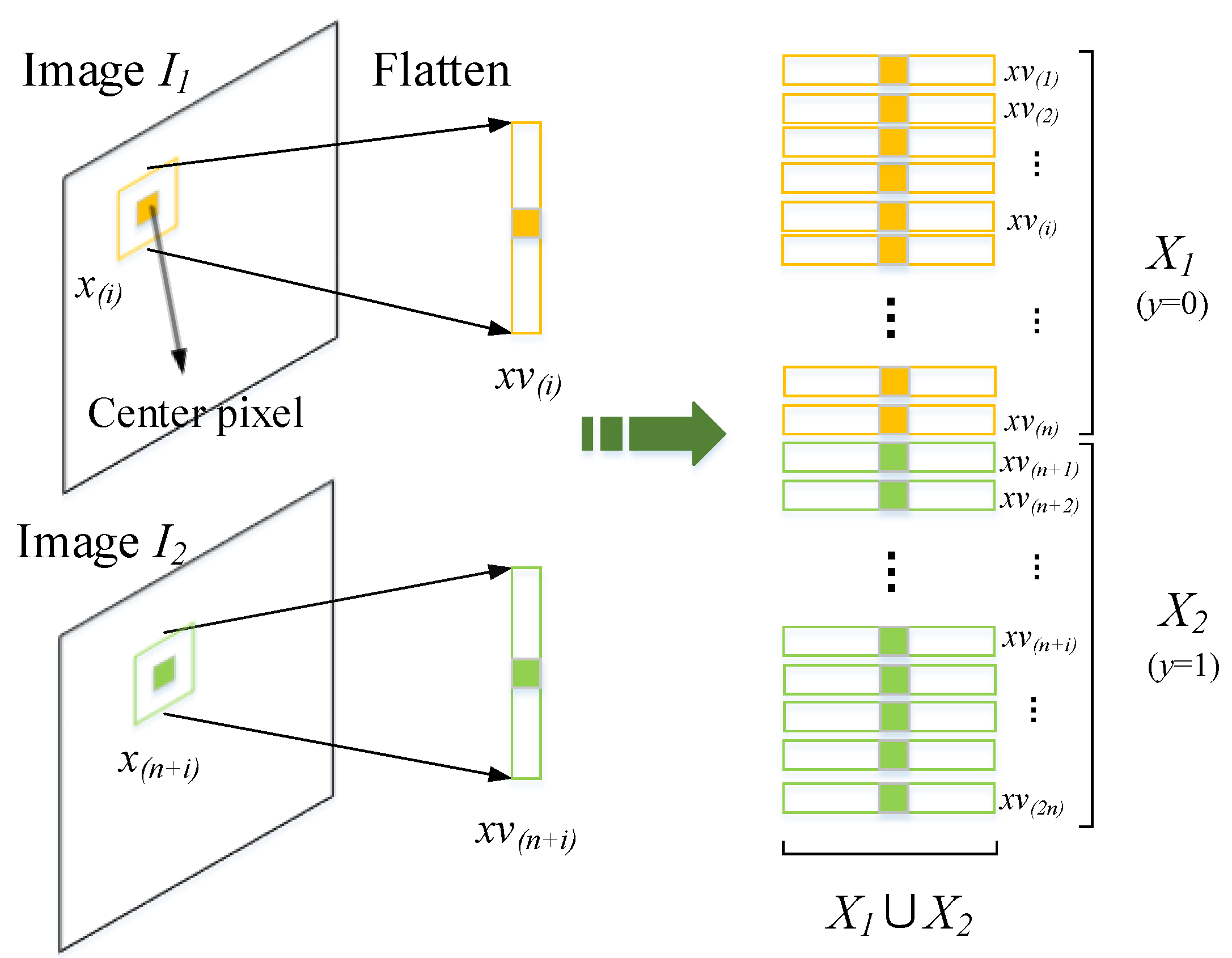
3.2. Architecture of Temporal Prediction

As our method derives from GAN, the proposed pretext task for learning representations is shown by analogy with it in Figure 4. Compared with the ordinary GAN, we do not require a Generator, differently from the GAN-based methods that use the entire model and focus on its generative property [54,55]. As mentioned above, we do not need to construct the generated data, when we assume $x_1^{land}$ is generated by G. Moreover, the $x_1^{land}$ “generated by the G” is already similar enough to the real sample $x_2^{land}$ (see Figure 3). Accordingly, we treat the samples from image $I_1$ as the fake data $X\left(fake\right)$ and the samples from image $I_2$ as the real ones $X\left(real\right)$. Only the D is trained to estimate the probability that a sample belongs to the real data distribution rather than the one generated by G. Thus, the network is equipped with the adversarial learning ability by training it to distinguish the sample x from image $I_1$ (i.e., the fake) rather than $I_2$ (i.e., the real). The discriminator $D(x;\theta )$ outputs the discriminative probability for each pixel, where $\theta$ represents the parameters of the discriminator. According to the discriminative target, x from image $I_1$ is labeled with $y=0$ and $I_2$ with $y=1$ (or reverse), such conditional probability $P(Y=y|x)$ is predicted by the D, where Y denotes which image source x comes from between images $I_1$ and $I_2$. By analogy with original GAN, this process can be viewed as a minimax discriminative adversarial game, which is actually contained in generative adversarial game of original GAN, i.e., the case of global optimality: G fixed and $p_g=p_{data}$. Our method is to leverage this case to learn representations based on the fact the common distribution between image pairs has enough similarity. Thus, we only need to train the D to converge to the optimal $D_G^{*}\left(x\right)$, the feature representation for given pixel neighborhood information can be obtained.

Furthermore, our model is completely equivalent to an optimal discriminator of a GAN for the case of common distribution in a sense, as it can be viewed as the situation G fixed and $p_g=p_{data}$. However, according to the specific characteristic of data in CD task, there is the case of non-common distribution, which can be viewed as a general classification task. Our model training for temporal prediction actually integrates the two cases into a unified discriminant framework. On the whole, compared to GAN, our model means that the optimal $D^{*}$ of GAN is generalized to the mixed cases of Cannot differentiate and Can differentiate for consistent feature mapping. Next, we will deal with the establishment, training, and result analysis of the proposed model.

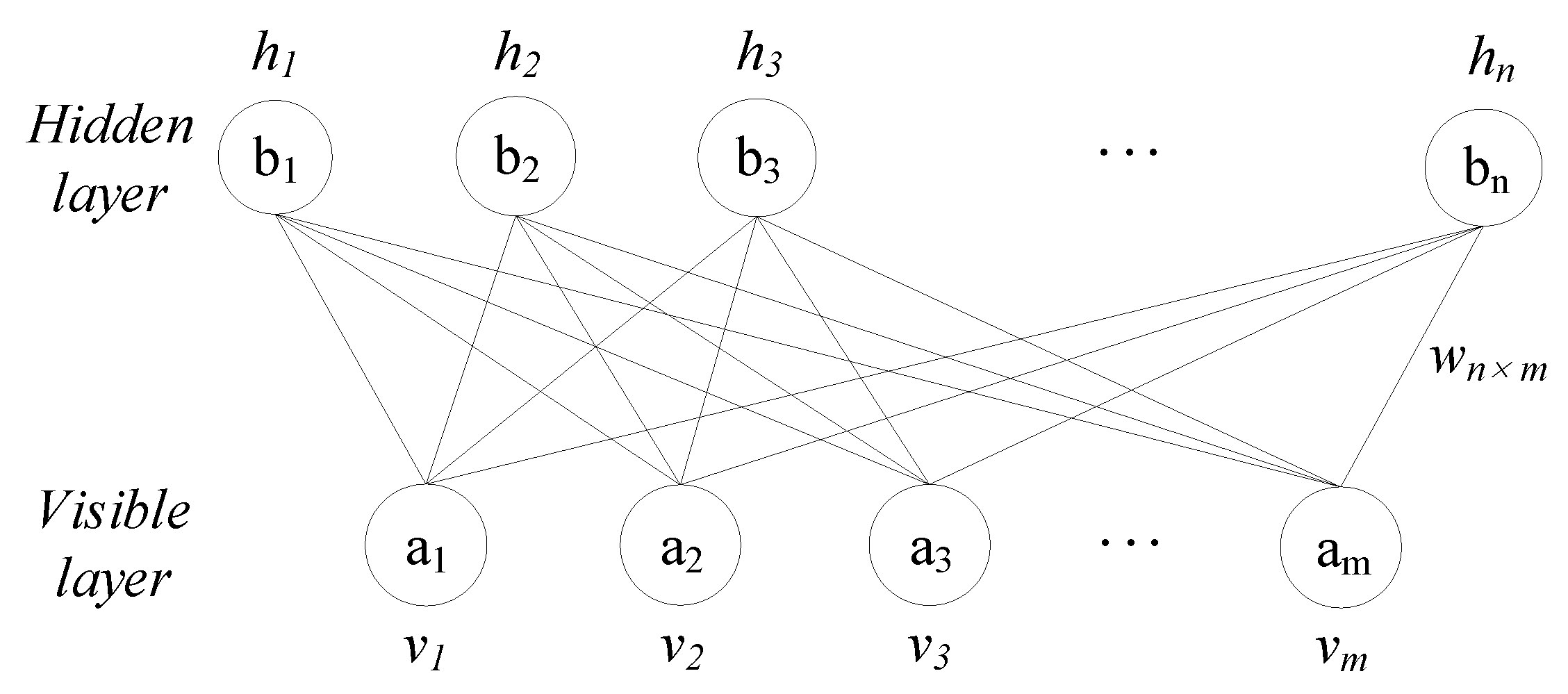
3.3. Establishment of Deep Neural Networks

Based on the mapping framework, the focus follows selecting a suitable discriminator rather than GAN-based whole generative model. What kind of network design is appropriate for our pretext task? Theoretically, it can be implemented via any discriminator model with back-propagation algorithms. Take these two points into account: (1) We assume the G fixed (i.e., have no G) from the beginning, only the D is trained, which means it cannot be improved and changed for the similarity of two-player as the networks training. (2) Due to the noises existed and fixed, the D may be able to distinguish the data source of similar samples that have a large difference in noise, if given enough training time. In case of heterogeneous images, our method is not directly applicable since the same ground material has distinct representations between image pairs. Our method is designed for homogeneous images and leverages the linear correlation of the intensity distribution between homogeneous image pairs, i.e, the same ground objects are represented similarly. This means our method is also not applicable to the cases of large illumination and seasonal variation. As a result, as our feature mapping mainly by Cannot differentiate, the D has no need for the strong recognition capacity. In computer vision community, the main neural network models include stacked autoencoders (SAEs) [62], deep belief networks (DBN) [63], and convolutional neural networks (CNN) [20]. They all can be trained to learn layer-by-layer features with similar hierarchical structure and nonlinear module. However, due to the nature of multiple hidden layers in the nonlinear deep model, there is the difficulty of optimizing the weights of the network. That means, with large or small initial weights, the networks both easily trap into the local optimum and hard to close to a satisfactory solution. Fortunately, previous work has shown the pretraining is able to alleviate this problem [38]. Therefore, we adopt the widely used deep neural networks (DNN) [50,59] as the desired discriminative model. It takes a two phases training strategy, one is unsupervised pretraining, other is supervised fine-tuning. Besides, SAEs consist of an encoder and a decoder, which are usually used for unsupervised image reconstruction. Compared to CNN, which can retain the spatial information of data for identifying, DNN is more promising to insure the validity and robustness of the proposed discriminative mechanism.

The restricted Boltzmann machines (RBMs) are the basal module for unsupervised pretraining process of the DNN [63,64]. As shown in Figure 5, an ordinary structure of RBM consists of two layers, in which one is the visible layer containing m visible units (denoted as $V=(v_1,...,v_m)$), and the other is hidden layer containing n hidden units (denoted as $H=(h_1,...,h_n)$) [65]. The units between different layers are connected to each other by the weight matrix $w_{n\times m}$. The units at the same layer have no connections. For a given joint state ($V,H$), the energy is defined as

$$E(V,H)=-\sum _{i=1}^m{a}_i{v}_i-\sum _{j=1}^n{b}_j{h}_j-\sum _{i,j}{v}_i{h}_j{w}_{ij}$$

(2)

where $w_{ij}\in w_{n\times m}$ is the weight between the visible unit $v_i$ and the hidden unit $h_j$, and $a_i$ and $b_j$ are their corresponding biases. The magnitude of this energy function guides the updating of the weights and biases.

The input data corresponds to the visible units, which are observed for their advanced features. Every hidden unit can be viewed as a feature detector. For the observed data V, the feature detector $h_j$ and the reconstructive visible unit $v_i$ have the states as

$$p(h_j=1|V)=\sigma (\sum _i^m{w}_{ij}{v}_i+b_j)$$

(3)

$$p(v_i=1|H)=\sigma (\sum _j^n{w}_{ij}{h}_j+a_i)$$

(4)

where $\sigma \left(x\right)=1/(1+exp(-x\left)\right)$ is the logistic sigmoid function. The states of the feature detectors are then calculated once more, which results in the features of the reconstruction. The weight is updated by the change:

$$\Delta w_{ij}=\mu ({\langle v_i{h}_j\rangle }_{ori}-{\langle v_i{h}_j\rangle }_{rec})$$

(5)

where $\mu$ is a learning rate, ${\langle v_i{h}_j\rangle }_{ori}$ is the expectation driven by original observed data, and ${\langle v_i{h}_j\rangle }_{rec}$ corresponds to the expectation of reconstruction. The biases are learnt by the same learning rule with a simplified version.

The learning of one RBM is performed as many times as desired, which constitutes the stacked RBM or deep belief networks (DBNs) [66]. Next, DNN are formed using the unfolding stacked RBM with the pretrained weights. Finally, a fine-tuning stage across the entire networks is applied, which minimizes the cross-entropy error:

$$E=-\sum _i{y}_{i}log\widehat{y_i}-\sum _i(1-y_i)log(1-\widehat{y_i})$$

(6)

where $y_i$ is the label of the training sample $x_i$, indicating the training sample $x_i$ come from image $I_1$ or image $I_2$, and $\widehat{y_i}$ is the predicted output and is also the final representations of raw input.

3.4. Training

As mentioned above, DNN is built based on a stack of RBM. The weights of multiple pretrained RBMs are used as the initial weights of DNN. Then, the entire network is fine-tuned using backpropagation. The DNN is capable of automatically discovering hierarchical representations by layer-wise learning directly from the observable data. For change detection, the high-level representations are the key to suppressing irrelevant variations and highlighting changes. We use the DNN to learn the high-level feature representation for CD by training for temporal prediction that asks the DNN to predict which temporal image a sample comes from. As similar samples can hardly be differentiated over their data source and thus will be competing each other, we term the instance based on DNN as discriminative adversarial deep neural networks (DADNN). Concretely, the proposed DADNN takes $X_1\cup X_2$ as input, where $X_1=\{x{v}_{\left(1\right)},x{v}_{\left(2\right)},...,x{v}_{\left(n\right)}\}$, $X_2=\{x{v}_{(n+1)},x{v}_{(n+2)},...,x{v}_{\left(2n\right)}\}$, n represents the number of pixels in an image, i.e., $n=W\times H$, $xv$ represents the flatten vector form of a sample patch x with the size $s\times s$ centered on a pixel, and $(·)$ represents the index of the sample for each pixel. The cross-entropy loss expressed as Equation 6 is minimized, where $y_i\in \{0,1\}$ and

$$y_i=\left\{\begin{array}{cc}0,\hfill & i\in (1,2,..,n)\hfill \\ 1,\hfill & i\in (n+1,n+2,...,2n)\hfill \end{array}\right.$$

(7)

That means $y_i=0$ denotes that the sample comes from image $I_1$; otherwise, the sample comes from image $I_2$ in the label sets shown in Figure 6. Because the mini-batch stochastic gradient descent (mini-SGD) algorithm is used in our experiments, such construction of training sets can be viewed as imitating a discriminator of a GAN that processes the fake (from $I_1$) and the real (from $I_2$) samples sequentially, i.e., alternately processing the real and the fake samples. This enables our network to be end-to-end and be easily implemented. So far, the corresponding high-level feature $f_i$ of a sample patch $x_i$ can be expressed as

$$f_i=D(x_i,\theta )$$

(8)

where D is the DNN that meanwhile can be as the learned mapping function, $\theta$ is weight sets of DNN, $f_i$ = $\widehat{y_i}$, i.e., the predicted output is the final learned features, which then are used to generate a DI by direct subtraction.

Different from most existing methods that process two adjacent units at the same position jointly, we treat two adjacent units at the same position as two samples to built the joint sample space with the number of $2n$. During the whole process, no matter at input or the top layer of the network, we have not joined them for learning, as our objective is discriminative adversarial mapping rather than learning a semantic classifier. Therefore, according to the discriminative objective, the labels are directly given as formulated in Equation (7), no need for additional work to produce available semantic labels. The learning procedure is formally presented in Algorithm 1.

Algorithm 1 Learning Procedure in DADNN

input:  Training samples $X_1\cup X_2=\{x{v}_{\left(1\right)},x{v}_{\left(2\right)},...,x{v}_{\left(n\right)},x{v}_{(n+1)},...,x{v}_{\left(2n\right)}\}$, testing samples $X_1$ and $X_2$. output:  $D\left(X_1\right)$ and $D\left(X_2\right)$, i.e., $F_1$ and $F_2$. 1: for number of training epochs do 2:     Sample minibatch of k samples $\{x{v}_{\left(1\right)},x{v}_{\left(2\right)},...,x{v}_{\left(k\right)}\}$ from $X_1\cup X_2$. 3:     Updating weights $\theta$ of the discriminator by minimizing the objective function in Equation (6) with given labels in Equation (7). 4: end for 5: After training, $X_1$ and $X_2$ are fed into the trained discriminator, respectively.

Via such discriminative adversarial learning by temporal prediction, the desired consistent feature representations $F_1=\left\{F_1(i,j)\right|1\le i\le W,1\le j\le H\}$ and $F_2=\left\{F_2(i,j)\right|1\le i\le W,1\le j\le H\}$ are obtained, which correspond to images $I_1$ and $I_2$, respectively. Because just a discriminator D is trained instead of training two networks G and D simultaneously, we do not face the problems of original GAN such as mode collapse and training instability. Therefore, the method presents stable training behavior in experiments. Moreover, unsupervised pretraining provides strong support for the proposed method to converge to satisfactory solutions.

3.5. Result Analysis

DADNN is trained to output a single probability for every x in image pairs. The probability indicates the data source of every x. At the same time, the probability is able to reveal a similarity metric for the distributions between two images as aforementioned, thus it can be used as the mapped high-level feature representations of raw image pairs. With the increase of discriminative ability of the networks, we would like the mapping result as shown in Figure 7, in which the joint distribution feature space is built, i.e., the distribution of the same type between two images is transformed into the consistent feature representations. Superficially, the probability of samples from $I_1$ is minimized ($y=0$) and simultaneously the probability of samples from $I_2$ is maximized ($y=1$). However, given there is no any position limitation, the actual adversarial two-player is the samples from the intensity distribution of the same types but different image source like the white and gray pixel blocks (see Figure 7). As aforementioned, as they belong to common distribution, the D hardly identifies their corresponding data source. The competing occurs between similar samples in image pairs. During the discriminative training process, when the abstract and discriminative features are extracted and the irrelevant variations are eliminated, the deep representations of similar samples from different images will become adversarial each other. In other words, for the common statistical distribution like the white and gray pixel blocks, they share similar feature representations between image pairs in deep feature space, the trained discriminator cannot differentiate their data source (i.e., come from $I_1$ or $I_2$). This is in accordance with optimizing goal of GAN.

Further, we denote the white parts for the intensity distribution $p_1$, the gray for $p_2$, the yellow for $p_3$, and the green for $p_4$. For $p_1$ and $p_2$, we have $p_{1,I1}=p_{1,I2}$ and $p_{2,I1}=p_{2,I2}$, and without a generator to train and generate, i.e., assume G fixed, which already satisfy the conditions of the global optimality in GAN’s minimax game from the beginning. Therefore, after several steps of training, the proposed discriminator has the certain capacity, it will converge where the discriminator cannot distinguish samples $x^{p1}$ from $x^{p2}$, i.e., $D^{*}\left(x^{p1}\right)=\frac{1}{2}$ and $D^{*}\left(x^{p2}\right)=\frac{1}{2}$. In practice, the specific output of the network is expressed as

$$\left\{\begin{array}{cc}\hfill & D\left(x^{p1}\right)=a_1\hfill \\ \hfill & D\left(x^{p2}\right)=a_2\hfill \\ \hfill & a_1,a_2\in (0,1),a_1\ne a_2,\mathrm{and}{a}_1,a_2\to \frac{1}{2}\hfill \end{array}\right.$$

(9)

where $a\to b$ denotes a closes to b. The D ultimately outputs the scalar $a_1$ for all samples from the intensity distribution $p_1$ and outputs another scalar $a_2$ for the samples from the intensity distribution $p_2$. With this, they are represented by more consistent features in the areas with the same statistical distribution. Furthermore, $D\left(x^{p1}\right)$ and $D\left(x^{p2}\right)$ close to the scalar $\frac{1}{2}$ from different directions as they belong to different statistical distributions. According to the Theorem 1 proof in [31], for $p_g=p_{data}$ and G fixed, the optimal discriminator has $D^{*}{}_G\left(x\right)=\frac{1}{2}$; it is not difficult to obtain the results above.

In addition, the samples $x^{p3}$ and $x^{p4}$ belong to the non-common statistical distribution between image pairs. It can be easily differentiated that $x^{p3}$ is from $I_1$ with $y=0$ and $x^{p4}$ is from $I_2$ with $y=1$, as a general classification task. Therefore, we can obtain the results as follows.

$$\left\{\begin{array}{cc}\hfill & D\left(x^{p3}\right)=a_3\hfill \\ \hfill & D\left(x^{p4}\right)=a_4\hfill \\ \hfill & a_3,a_4\in (0,1),a_3\ne a_4,a_3\to 0,\mathrm{and}{a}_4\to 1\hfill \end{array}\right.$$

(10)

It is worth emphasizing that, differently from the case of common distribution, there is no competition between the samples from non-common one. Their identification probability will close to their given labels.

3.6. Mapping-Based Binary Segmentation

After training over DADNN, the neighbor vector of every pixel in image pairs $I_1$ and $I_2$ is fed into the network again, the consistent features $F_1$ and $F_2$ are obtained as discussed above. The two transformed feature maps represent the two original images well. The key issue of generating DI is to suppress the information of unchanged areas and strengthen the information of changed areas. Next, such DI is calculated by direct comparison pixel by pixel based on these two feature maps as

$$F_d(i,j)=|F_1(i,j)-F_2(i,j)|$$

(11)

where $F_d$ denotes the DI. Finally, in order to avoid the influence of possible outliers, we use FCM algorithm with local neighbor ($3\times 3$ pixels) to segment $F_d$ into two classes, i.e., the changes and unchanges, and obtain the binary change map.

4. Experimental Study

In this section, we first investigate the proposed discriminative adversarial mechanism, and then display the performance of the proposed method by reporting the experimental results and numerical evaluations on remote sensing images. Finally, the effects of noises and the related parameters are analyzed.

Our codes are written in Matlab language. The environment of running codes is shown as follows, Intel(R) Core(TM) i5-6500M CPU @ 3.20GHz 3.20GHz, RAM:8.00GB, Windows7 Pro (64-bit) and Matlab R2016b.

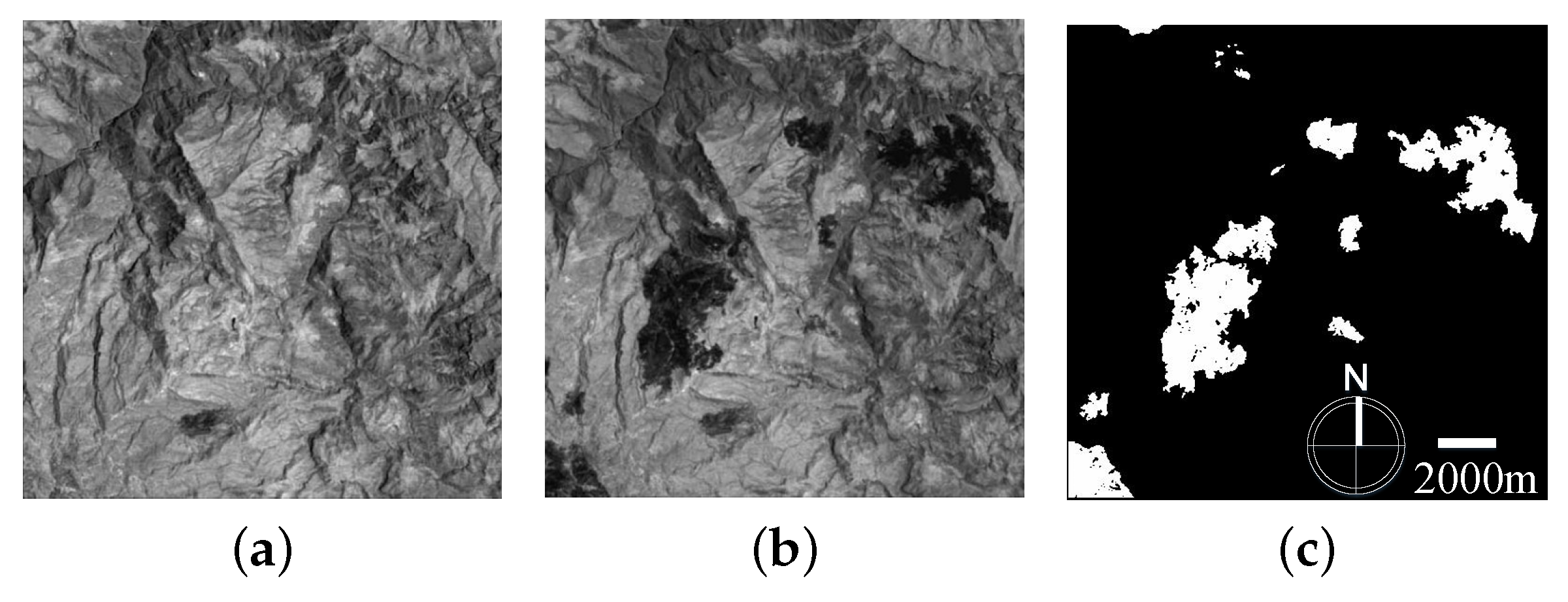
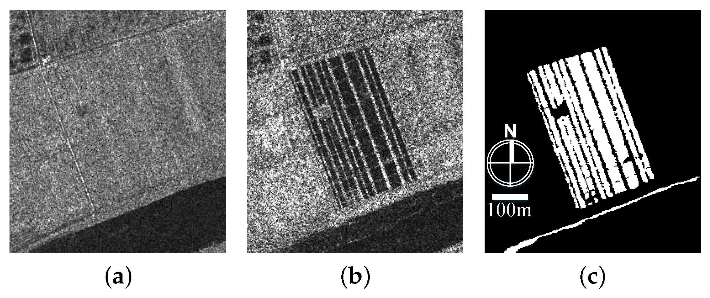
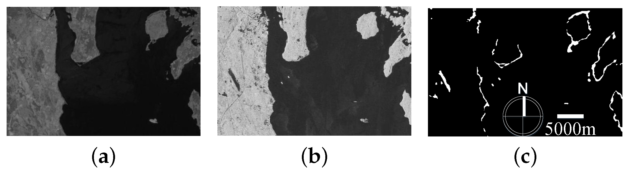
4.1. Data Description

Mexico dataset: The data set consists of two optical images ($512\times 512$ pixels) acquired by Landsat-7 (US satellite) at urban Mexico in April 2000 and May 2002, respectively. These two images are extracted from the Band 4 of the ETM+ images. This data set shows the vegetation damage after the forest fire at urban Mexico as depicted in Figure 8a,b. Figure 8c shows the reference image, which represents the changed areas.

Ottawa dataset: The data set is a section ($290\times 350$ pixels) of two SAR images over the city of Ottawa acquired by RADARSAT SAR sensor. They were provided by the Defence Research and Development Canada, Ottawa. This data set contains two images acquired in July and August 1997 and presents the areas once afflicted with floods. The images and the available reference image are shown in Figure 9a–c, in which panel (c) is created by integrating prior information with photo interpretation.

Yellow River dataset: The data set used in the experiments consists of two SAR images ($257\times 289$ pixels) as shown Figure 10a,b. The representative section is selected from two huge SAR images acquired by Radarsat-2 at the region of the Yellow River Estuary in China in June 2008 and June 2009. Their original size is $7666\times 7692$. The available reference image of the selected areas is presented in Figure 10c, which is created through integrating prior information with photo interpretation based on the input images. It is worth noting that the two images are a single-look and four-look image, respectively. This means that the influence of speckle noise on the image acquired in 2008 is much greater than the one acquired in 2009. Such huge discrepancy of speckle noise distribution between the two images may complicates the processing of change detection.

Campbell River dataset: The data set consists of a segment from the HH mode (L-band) of a scene taken by the sensor ALOS-PALSAR on June 2010, at the region of Campbell River in British Columbia (with an initial spatial resolution of 15 m resampled to 30 m) and of a segment with a size of $800\times 800$ pixels from band 5 (1.55–1.75 $\mathsf{\mu }$m) of a scene taken by the sensor Landsat Enhanced Thematic Mapper Plus (ETM+) on June 1999, at the same region (with a spatial resolution of 30 m). The two SAR images and corresponding reference image of the size of $505\times 336$ are shown in Figure 11a–c.

4.2. Experimental Setup

(1). General information in comparison. In order to validate the effectiveness of the proposed DADNN method, six closely related algorithms were implemented as comparison: subtraction, log-ratio operator, wavelet fusion [17], DNN [38], SSCNN [51], and SCCN [30]. The parameters of DNN, SSCNN, and SCCN methods are set up by default in [30,38,51]. In DNN, the neighbor size is set to 5, and $\alpha =0.7$ is selected as mentioned in [38]. In SSCNN, the neighborhood size is set to 9. In SCCN, $\lambda =0.02$ is selected as mentioned in [30]. Besides, the impact of the neighborhood size on the method is not investigated, we set it to 5. In these methods referring to DI-generation, i.e., subtraction, log-ratio operator, wavelet fusion, SCCN, and the proposed DADNN, FCM algorithm with $3\times 3$ neighborhood information instead of a single pixel is used to cluster their DIs into binary maps. Moreover, in the proposed DADNN, for all data sets, we use $s\times s$-100-50-1 network based on lots of experimental investigation, where s represents the size of neighborhood. As aforementioned, the mini-batch stochastic gradient descent (mini-SGD) algorithm is used in our experiments. We set the weight decay parameter to 1 in L2 regularization for optical grayscale image, 0 for multispectral and SAR images. The learning rate is usually adjusted by 1.

(2). Evaluation criteria: We use the false positives (FP), false negatives (FN), overall error (OE), percentage correct classification (PCC), and Kappa coefficient (Kappa) [67] to quantitatively evaluate the performance of the detection result. Moreover, the quality of DIs is quantitatively evaluated by the receiver operating characteristics (ROC) plot and the area under curve (AUC) of ROC [68]. For a high-quality DI, the ROC plot should be close to the top-left corner of the coordinate system. The larger AUC value shows a higher quality of the DI. The AUC value equals to 1 signifies a perfect DI.

4.3. Verification of Theoretical Results and Feature Visualization Analysis

This experiment is made for verifying whether correct the theoretical results of DADNN and simultaneously analyzing the learned feature maps. As shown in Figure 12a,b, the Ottawa data set consists of intensity distributions of two types, i.e., water and land. Through the feature learning of DADNN, the two distributions are regulated to two different probabilities and both are nearby $\frac{1}{2}$ (see Figure 12g,h). The differences between intensity distributions of the same types are minimized. Obviously, the black areas represent the water and white areas represent the land as shown in Figure 12c,d. It can be observed the irrelevant variations between the image pair are eliminated remarkably, the transformed high level representations have the remarkable consistency for the two images. However, the optical Mexico data set are regulated slightly (see Figure 13). It seems that the background of the transformed feature maps is brighter and increase the overall contrast than the original images. Usually, owing to the existence of speckle noises, SAR images are more complex and difficult to handle than the optical ones. However, it can be seen the performance of DADNN on SAR images is better than the optical ones. This is partly because the existence of speckle noises can disturb the discrimination of the networks so that achieve a better feature mapping result. Furthermore, the optical Mexico data set has very diverse ground features, which is more complex for our minimax adversarial game. As a result, DADNN still increases the consistency between two optical images for direct comparison. As shown in

Table 2. Value of evaluation criteria of the Mexico data set.

Method	AUC	FP (%)	FN (%)	OE (%)	PCC (%)	Kappa (%)
subtraction	0.9868	0.38	1.42	1.80	98.20	89.23
log-ratio	0.9874	0.27	2.18	2.45	97.55	84.75
wavelet fusion	0.9885	0.89	0.85	1.74	98.26	90.14
DNN	-	0.18	2.67	2.85	97.15	81.72
SSCNN	-	0.38	1.50	1.88	98.12	88.78
SCCN	0.9883	0.42	1.31	1.73	98.27	89.76
DADNN	0.9961	0.69	0.74	1.43	98.57	91.86

, the quantitative evaluations manifest DADNN has the capacity of further improving detection accuracy. Although it did not achieve the ideal theoretical results, the background got visually suppressed to some extent. Furthermore, the verification for the case of common distribution are shown clearly here (see Figure 12), the non-common case is further verified in Appendixes Appendix A.1 and Appendix A.2. In Appendix A.3, we further investigate whether the DADNN performs better on feature mapping when Gaussian noise is applied to the optical Mexico data set.

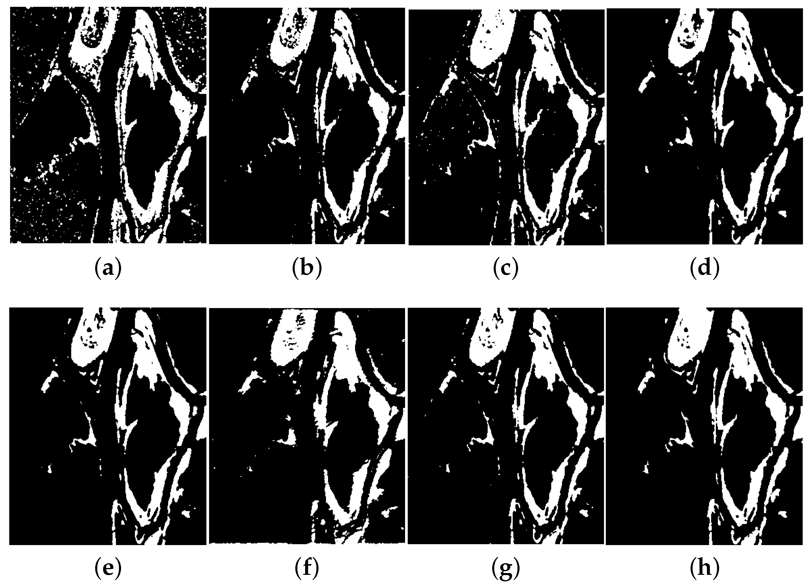
4.4. Performance of Detection Results

Mexico dataset: The Mexico data set is optical images in grayscale, which are usually easier than SAR images for change detection because the speckle noises and outliers in SAR images are hard to handle. The optical image pairs possess the adversarial characteristic as discussed in Section 3.1, so we first measure the utility of the proposed method in optical images. The DIs generated by different algorithms are shown in Figure 14. The subtraction operator and log-ratio operator are usually carried out. The subtraction operator can highlight the changed areas, but the background cannot be suppressed. The log-ratio operator suppresses the complex background, but it fails to highlight the changed areas (see the enlarged details in the second row of Figure 14a). The wavelet fusion based method fuses log-ratio and mean-ratio images. It retains the more changed information, but the background noises and complicated topography are not effectively suppressed. The SCCN method uses a probability map to guide the fine-tuning of network parameters in unchanged pixels. Therefore, it suppresses some background disturbance, but it cannot obviously highlight the changed areas. The proposed DADNN method does not dramatically obtain the ideal result in vision due to the abundant optical textual features. However, as illustrated in Figure 15, the ROC plots for the five DIs show the DADNN outperforms the other four methods in comparison, which indicates the proposed adversarial feature learning has increased the consistency between the image pairs for effective difference representations. The DNN and SSCNN based methods directly generate the final detection result without the generation of DI. As there is a good consistency between the two images, the minor fine-tuning is sufficient for more consistent feature representations. Thus, the weight decay parameter is set to 1 for this dataset.

Next, the FCM algorithm with adjacent information is used to segment the five DIs. Figure 16 shows the binary detection results. The used FCM method integrates the spatial contextual information. Therefore, it can restrain outliers to some extent. All compared methods obtained the good performance for the segmented results. However, as it can be observed in the change maps obtained by compared methods, some white noise spots still exist. By contrast, the proposed method applying adversarial learning has an improvement in reducing background noises and retaining more changed details. Moreover, quantitative evaluations in Table 2 also confirm this point. For compared methods, the false alarms are high, and the missed alarms are low. This is especially for the result obtained by the DNN method, which yields the lowest FP of 0.18% and the highest FN of 2.6%, as DNN method suffers from the error accumulations of an initial change map and sample selection. Benefited by CNN, SSCNN has a large robustness to coarse pseudo-labels. Moreover, no sample selection increases the diversity of samples. Therefore, SSCNN yields the lower OE of 1.88% than DNN with the OE of 2.85%. The effect of the proposed DADNN on transforming features is better and can more effectively suppress the irrelevant variations than SCCN method. The best Kappa of 91.86% is yielded by the proposed method.

Ottawa dataset: For the Ottawa data set, the DIs produced by the proposed algorithm and the compared methods are shown in Figure 17. The performance of the subtraction operator is the worst. It severely misses the changed details and the land part in the background is seriously polluted by white noise spots. The log-ratio operator transforms the multiplicative speckle noises into the additive one, so it suppresses background noise. However, the enlarged detail in the second row of Figure 17b shows changed information is not highlighted. The wavelet fusion is good in keeping changed detail information, but it cannot suppress well the unchanged information shown in Figure 17c. Owing to SCCN method extracting the high-level features, it suppresses the background noises to some extent. However, it does not consider the changed pixels, which results in a high missing of changed details shown in Figure 17d. By contrast, the proposed DADNN can greatly highlight the changed areas and suppress the noises well. The details displayed in the second row of Figure 17e obviously indicate this point. Figure 18 also shows the proposed method produces the best DI. The wavelet fusion based method follows closely the proposed method. Because DADNN is less affected by additional factors such as manual parameter, the performance of feature mapping is superior to other algorithms.

After these DIs are classified by FCM method, respectively, the detection results including ones acquired by DNN- and SSCNN-based methods are presented in Figure 19.

Table 3. Value of evaluation criteria of the Ottawa data set.

Method	AUC	FP (%)	FN (%)	OE (%)	PCC (%)	Kappa (%)
subtraction	0.9103	5.68	2.40	8.08	91.92	72.00
log-ratio	0.9576	0.58	1.86	2.44	97.56	90.52
wavelet fusion	0.9907	1.89	0.20	2.09	97.91	92.49
DNN	-	0.19	1.96	2.15	97.85	91.58
SSCNN	-	0.57	1.24	1.81	98.09	93.08
SCCN	0.9609	1.56	1.95	3.51	96.49	86.69
DADNN	0.9945	0.39	1.17	1.56	98.44	94.02

reports the quantitative evaluations. The change map obtained by subtraction operator has many white noise spots due to image speckle noises, and much changed information has not been detected compared to the reference image. Therefore, subtraction operator yields the highest OE of 8.08%. The log-ratio method suppresses the noises but misses some changed details. The wavelet fusion produces the lowest FN of 0.20%, which reveals the more changed details than other methods. However, it does not accurately reveals unchanged areas. As DNN, SSDNN, and SCCN are based on feature learning, they are robust to speckle noises. By contrast, the proposed DADNN yields the best balance between suppressing the noises and highlighting the changed information. The highest AUC is 0.9945 and the highest Kappa is 94.02%, which are yielded by DADNN. As the purpose of DADNN is minimizing the discrepancy between two images, it provides a great basis for further direct comparison.

Yellow River dataset: For this data set, the speckle noise has a greater impact on the single-look image captured in 2008 than on the four-look image captured in 2009 as mentioned above. That means accurately detecting changes is more difficult than on the first two data sets. The DIs obtained by different algorithms are shown in Figure 20. The proposed DADNN obviously highlights the changed areas and suppresses the background noises. The subtraction operator is very sensitive to speckle noises. It does not correctly reveal the changed information, which is swarmed with dense noises. The log-ratio operator is robust to speckle noises, thus making the changed areas quite obscure. It can be observed the DI generated by wavelet fusion retains the changed areas well, however, the background noises are less effectively suppressed. SCCN method suppresses some background noises, but more changed details have not been detected. The ROC curve of DADNN is the nearest to the top-left corner of the coordinate system (see Figure 21a), which means the DI generated by DADNN is the best. The final segmented maps are shown in Figure 22. These intensity-based approaches—subtraction, log-ratio, and wavelet fusion—cannot reveal the unchanged areas well due to image inconsistency especially for speckle noises. The feature-based methods DNN, SSCNN, SCCN, and DADNN are more effective in suppressing the background noises and revealing the changed information. However, DNN, SSCNN, and SCCN cannot do better than DADNN.

Table 4. Value of evaluation criteria of the Yellow River data set.

Method	AUC	FP (%)	FN (%)	OE (%)	PCC (%)	Kappa (%)
subtraction	0.6570	37.18	3.78	40.96	59.04	19.60
log-ratio	0.7639	22.03	1.72	23.75	76.25	44.25
wavelet fusion	0.8520	17.46	2.26	19.72	80.28	49.86
DNN	-	0.67	5.95	6.62	93.38	74.77
SSCNN	-	0.66	4.46	5.12	94.88	81.16
SCCN	0.9328	7.06	2.41	9.47	90.53	70.96
DADNN	0.9621	2.21	2.23	4.44	95.56	85.01

shows the DADNN yields the lowest OE of 4.44%, and the highest AUC, PCC, and Kappa of 0.9621, 95.56%, and 85.01%, respectively. The DADNN method contributed by adversarial feature learning is robust to speckle noises and retains the more changed information, so it provides a more accurate detection than other methods.

Campbell River dataset: If the dissimilarity in the Yellow River data set is caused by speckle noise, the inconsistency for the Campbell River data set is mainly the difference of brightness. It is very difficult for detection methods to correctly reveal changed areas in this dataset. As shown in Figure 23 and Figure 24a–c, these methods (subtraction, log-ratio, and wavelet fusion) without feature transformation are out of operation. The changed information is incorrectly detected. All of them are sensitive to the brightness variation. DNN and SSCNN also do not reveal the changed areas correctly, since they suffer from the error accumulation of traditional methods. Conversely, the SCCN and DADNN methods based on feature transformation learning correctly reveal the changed areas. However, the change detection result generated by SCCN is coarse and a part of unchanged areas is badly polluted by white noises. The quantitative evaluations are presented in Figure 21b and

Table 5. Value of evaluation criteria of the Campbell River data set.

Method	AUC	FP (%)	FN (%)	OE (%)	PCC (%)	Kappa (%)
subtraction	0.7527	64.09	0.13	64.22	35.78	2.32
log-ratio	0.8245	58.77	0.13	58.90	41.10	2.98
wavelet fusion	0.8711	54.05	0.13	54.18	45.82	3.68
DNN	-	59.47	0.03	59.50	40.50	3.20
SSCNN	-	58.77	0.10	58.86	41.14	3.10
SCCN	0.8901	15.17	0.56	15.73	84.27	17.40
DADNN	0.9522	3.17	0.48	3.65	96.35	52.89

. The proposed DADNN method significantly outperforms compared methods. The Kappa yielded by DADNN is 35.49% higher than the one from SCCN. Subtraction operator yields the very low Kappa of 2.32%. DNN achieves the lowest FN of 0.03% but the high FP of 59.47%. The DADNN not only correctly reveals the changed areas but also effectively reduces the noises, while overcoming the large difference in brightness. Due to the learning with adversarial mechanism has less dependency, the robustness to the inconsistency especially in brightness is better than other methods.

More experimental results can be found in Appendix B.

4.5. Effect of Noise

As described previously, the accurate pixelwise difference between remote sensing images is difficult to obtain due to the irrelevant variations caused by the property of sensors or complicated environment. The typical corruption is often from the noises according to different types of sensors. For example, optical images often suffer from additive noise and SAR images often are polluted by the speckle noises. Different from the additive noises, speckle noise is a type of multiplicative, uniformly distributed random noise. The unsupervised adversarial learning can automatically capture the helpful and abstract feature representations from corrupted input. It can be utilized to relieve the inconsistencies and suppress the noise corruption for CD. Therefore, in order to test the influence of different noises on DADNN, we apply different levels of Gaussian noise (a type of additive noise) and Speckle noise to the four data sets and evaluate DADNN using AUC values of the generated DIs. Figure 25 shows the variation of AUC values for the different levels of the different noises. The DADNN is more robust to Speckle noises than Gaussian noises. With the increase of the noise variance, the AUC values decrease dramatically when Gaussian noises is applied to the raw image data, whereas the AUC values decrease very slowly when Speckle noise is applied. Besides, AUC values on the Yellow river data set almost have not declined even though the images are polluted very badly by Speckle noise. Especially, the AUC value with the variance 0.05 of Speckle noise equals 0.9645, which is slightly better than one 0.9621 when no noise is applied. As it can be observed from Figure 26, it is easier for the networks to learn simple Gaussian white noises than Speckle noise. As the pollution of Gaussian noise is worse and worse, the networks only learnt the more Gaussian noise especially in simple texture areas. Eventually, just the rough distribution profile can be observed. Inversely, the multiplicative Speckle noise is not easy to learn by the networks, and thus it reaches the desired adversarial effects as well as the better performance of generating DI. These results are in agreement with our initial analysis: when cannot differentiate, the networks put similar samples into the same category and close the gap between them.

4.6. Analysis of Parameters

In this section, we further study the influences of neighborhood size and network structure on the performance of the proposed method. Besides, the weight decay parameter can be selected from 0 or 1 in our method, it is easy to set this parameter.

4.6.1. Effects of Neighborhood Size

The size s of neighborhood influences the performance of DADNN. Besides, except for the hyperparameters of the networks, no any other manual parameter is introduced. Therefore, we make a sensitivity analysis on the size s of neighborhood. We set s to 3, 5, 7, and 9 to investigate its influence on PCC and Kappa for four data sets. As shown in Figure 27, the DADNN in the optical images (i.e., Mexico data set) is less sensitive to the values of s than in SAR images. For SAR images, the curve of PCC has a relatively large fluctuation. The degree of discrepancy between two images may determine the suitable value of s. When the discrepancy is too big between two images especially in Campbell River data set, the small value of s is inadequate for the networks to learn the useful feature representations and discriminate the difference between the samples. However, if s is large, i.e., over 7, the neighborhood information is too redundant and has a low correlation with the corresponding center pixel, which leads to an improper network fine-tuning by means of the totally unsupervised manner, and the boundary detail information is more lost. Setting $s=3$ or $s=5$ are better choices for the first three data sets. Setting $s=7$, the results are the best for the last data set.

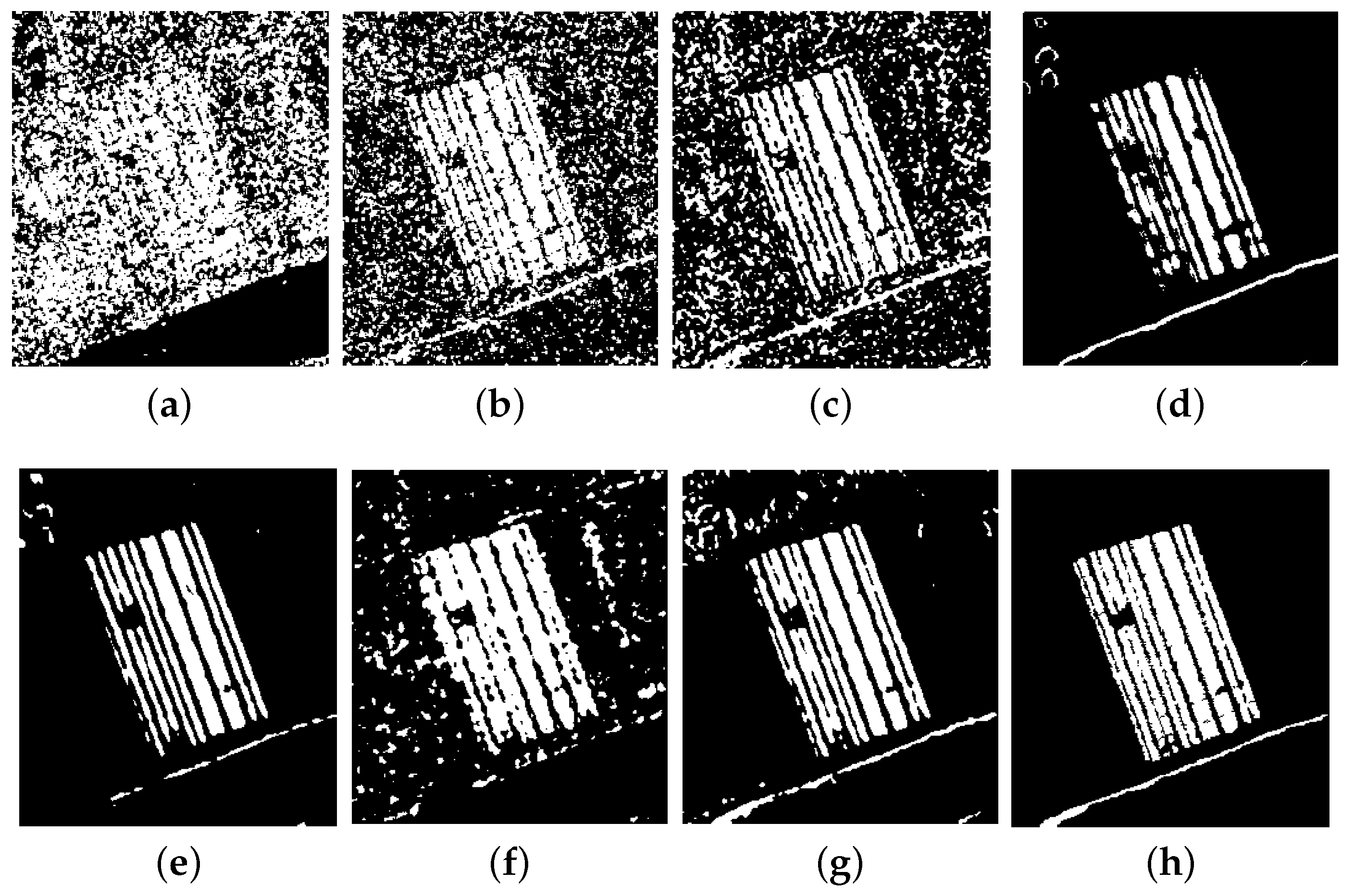
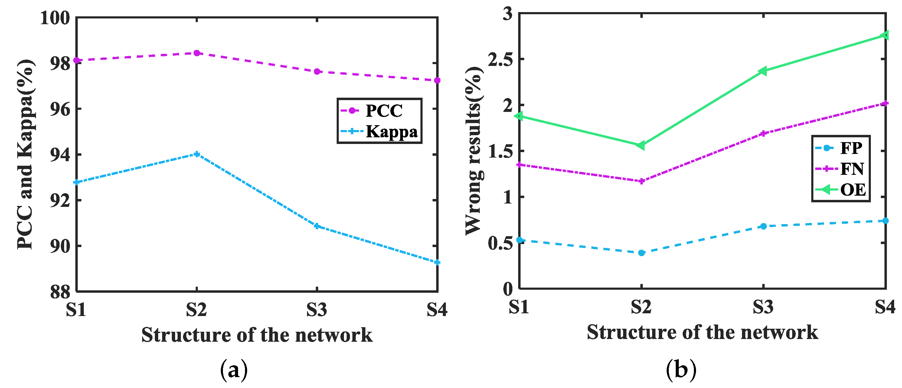
4.6.2. Effects of Network Structure

Network structure plays an important role in our discriminative adversarial feature mapping. We survey the effect of different structures on detection results in Ottawa data set. The relationship between the network structure and the criteria on Ottawa data set is shown in Figure 28. The lower values of FP, FN, and OE as well as higher values of PCC and Kappa are achieved by the structure S2, i.e., 9-100-50-1. The deeper and shallower networks both perform poorly. The deeper networks learn more abstract and discriminative features, which are not robust enough to the irrelevant variations. With more hidden layers, the lower PCC and Kappa values and the higher FP, FN and OE values are yielded. The theoretical effect is the samples from the same statistical distribution can not be identified so that they can be aligned for the same scalar by the discriminator. If the networks are too shallow, they are not adequate to capture the useful and hierarchical feature representations for discrimination. By contrast, the results obtained by the structure S2 (9-100-50-1) are the best as we analyzed in Section 3.3.

4.7. Discussion

For DADNN, it only consists of a discriminator based on DNN, and there is no need for additional steps to obtain available labels. In terms of this, the proposed method has a lower time and computational complexities than most existing methods that need prior knowledge from the semantic labeled data. Compared other fields such as image classification with ImageNet database, the field of CD has always facing the problem of the lack of accurate labeled samples, which limits the ability and widespread use of the labeled data-driven deep network for CD. Our method alleviates the problem very well. As it does not depend on changed and unchanged prior knowledge and breaks the limitation of semantic supervision, our method performs better than compared methods on some images. The main drawback of the proposed method is that it is not sensitive to small changed areas and the final result is affected by the quality of extracted features. The former is a common problem in most existing methods. Due to the promising and instructive results of our proposed approach, it deserves to be studied.

5. Conclusions

In this paper, a novel self-supervised algorithm is proposed for remote sensing image CD. Based on the imaging characteristic of homogeneous images, we regard learning useful representations as an unusual identifying problem, i.e., temporal prediction, for CD. We utilize the work mechanism of GAN’s discriminator (without a generator) to build a discriminative adversarial deep neural networks (DADNN). The discriminative networks are trained to differentiate samples from bitemporal images. Different from most existing methods that depend on predetection to learn the latent pattern between changed and unchanged classes, the proposed DADNN learns robust features in a completely unsupervised manner, without using any prior information over changes and unchanges. For homogeneous images, the same ground object has the same statistical distribution. Therefore, the discriminator hardly distinguishes image sources (from image $I_1$ or $I_2$) of the samples from the same distribution. We model this as a discriminative adversarial game to build the joint feature space of distribution. The principle is similar to human discrimination between two similar samples: we think they belong to the same class when they are indistinguishable, and give the probability $\frac{1}{2}$ of random guessing. Meanwhile, the discriminator can differentiate unique distribution between two images with probabilities 0 or 1. Therefore, in the joint feature space of distribution, two input images are transformed into more consistent feature representations by mapping the intensity distribution of the same type into an identical probability. Based on two consistent feature maps, the accurate detection is simplified only by direct comparison and FCM segmentation.

Experimental results on real remote sensing datasets demonstrate the effectiveness and potential of the proposed algorithm, which exhibits good performance on reducing the irrelevant variations and highlighting changes, especially for image pairs with large-scale ground objects. In the future work, we will consider adapting our method to other homogeneous remote sensing images such as hyperspectral images. We will also consider developing other better unsupervised CD methods with powerful deep learning.

References

1. Singh, A. Review Article Digital change detection techniques using remotely-sensed data. Int. J. Remote. Sens. 1989, 10, 989–1003. [Google Scholar] [CrossRef] [Green Version]
2. Saxena, R.; Watson, L.T.; Wynne, R.H.; Brooks, E.B.; Thomas, V.A.; Zhiqiang, Y.; Kennedy, R.E. Towards a polyalgorithm for land use change detection. J. Photogramm. Remote Sens. 2018, 144, 217–234. [Google Scholar] [CrossRef]
3. Xing, J.; Sieber, R.; Caelli, T. A scale-invariant change detection method for land use/cover change research. J. Photogramm. Remote Sens. 2018, 141, 252–264. [Google Scholar] [CrossRef]
4. Gong, J.; Ma, G.; Zhou, Q. A review of multi-temporal remote sensing data change detection algorithms. Protein Expr. Purif. 2011, 82, 308–316. [Google Scholar]
5. Bruzzone, L.; Prieto, D.F. Automatic analysis of the difference image for unsupervised change detection. IEEE Trans. Geosci. Remote Sens. 2000, 38, 1171–1182. [Google Scholar] [CrossRef] [Green Version]
6. Huerta, I.; Pedersoli, M.; Gonzalez, J.; Sanfeliu, A. Combining where and what in change detection for unsupervised foreground learning in surveillance. Pattern Recognit. 2015, 48, 709–719. [Google Scholar] [CrossRef] [Green Version]
7. Ghanbari, M.; Akbari, V. Generalized minimum-error thresholding for unsupervised change detection from multilook polarimetric SAR data. IEEE Trans. Geosci. Remote. Sens. 2015, 44, 2972–2982. [Google Scholar]
8. Zanetti, M.; Bruzzone, L. A Theoretical Framework for Change Detection Based on a Compound Multiclass Statistical Model of the Difference Image. IEEE Trans. Geosci. Remote Sens. 2018, 56, 1129–1143. [Google Scholar] [CrossRef]
9. Ferretti, A.; Montiguarnieri, A.; Prati, C.; Rocca, F.; Massonet, D. InSAR Principles–Guidelines for SAR Interferometry Processing and Interpretation. J. Financ. Stab. 2007, 10, 156–162. [Google Scholar]
10. Ban, Y.; Yousif, O. Change Detection Techniques: A Review; Springer International Publishing: Berlin/Heidelberg, Germany, 2016. [Google Scholar]
11. Tewkesbury, A.P.; Comber, A.J.; Tate, N.J.; Lamb, A.; Fisher, P.F. A critical synthesis of remotely sensed optical image change detection techniques. Remote Sens. Environ. 2015, 160, 1–14. [Google Scholar] [CrossRef] [Green Version]
12. Lunetta, R.S.E.; Christopher, D. Remote Sensing Change Detection: Environmental Monitoring Methods and Applications; CRC Press: Boca Raton, FL, USA, 1998. [Google Scholar]
13. Gong, M.; Li, Y.; Jiao, L.; Jia, M.; Su, L. SAR change detection based on intensity and texture changes. J. Photogramm. Remote Sens. 2014, 93, 123–135. [Google Scholar] [CrossRef]
14. Bovolo, F.; Bruzzone, L. A theoretical framework for unsupervised change detection based on change vector analysis in the polar domain. IEEE Trans. Geosci. Remote Sens. 2006, 45, 218–236. [Google Scholar] [CrossRef] [Green Version]
15. Celik, T. Unsupervised Change Detection in Satellite Images Using Principal Component Analysis and k-Means Clustering. IEEE GEoscience Remote Sens. Lett. 2009, 6, 772–776. [Google Scholar] [CrossRef]
16. Sezgin, M.; Sankur, B.L. Survey over image thresholding techniques and quantitative performance evaluation. J. Electron. Imaging 2004, 13, 146–166. [Google Scholar]
17. Gong, M.; Zhou, Z.; Ma, J. Change detection in synthetic aperture radar images based on image fusion and fuzzy clustering. IEEE Trans. Image Process. 2012, 21, 2141. [Google Scholar] [CrossRef]
18. Zhao, W.; Wang, Z.; Gong, M.; Liu, J. Discriminative Feature Learning for Unsupervised Change Detection in Heterogeneous Images Based on a Coupled Neural Network. IEEE Trans. Geosci. Remote Sens. 2017, 55, 7066–7080. [Google Scholar] [CrossRef]
19. Mikolov, T.; Kombrink, S.; Burget, L.; Cernocky, J.; Khudanpur, S. Extensions of recurrent neural network language model. In Proceedings of the IEEE International Conference on Acoustics, Speech and Signal Processing, Prague, Czech Republic, 22–27 May 2011; pp. 5528–5531. [Google Scholar]
20. Krizhevsky, A.; Sutskever, I.; Hinton, G.E. ImageNet classification with deep convolutional neural networks. In Proceedings of the Advances on Neural Information Processing Systems, Lake Tahoe, NV, USA, 3–6 December 2012; pp. 1097–1105. [Google Scholar]
21. Dai, J.; Li, Y.; He, K.; Sun, J. R-FCN: Object Detection via Region-based Fully Convolutional Networks. In Proceedings of the Advances on Neural Information Processing Systems, Barcelona, Spain, 5–10 December 2016; pp. 379–387. [Google Scholar]
22. Song, Y.; Ma, C.; Wu, X.; Gong, L.; Bao, L.; Zuo, W.; Shen, C.; Lau, R.W.; Yang, M.H. Vital: Visual tracking via adversarial learning. In Proceedings of the IEEE Conference on Computer Vision and Pattern Recognition, Salt Lake City, UT, USA, 18–23 June 2018; pp. 8990–8999. [Google Scholar]
23. Radford, A.; Metz, L.; Chintala, S. Unsupervised Representation Learning with Deep Convolutional Generative Adversarial Networks. arXiv 2015, arXiv:1511.06434. [Google Scholar]
24. Isola, P.; Zhu, J.Y.; Zhou, T.; Efros, A.A. Image-to-image translation with conditional adversarial networks. In Proceedings of the IEEE Conference on Computer Vision and Pattern Recognition, Honolulu, HI, USA, 21–26 July 2017; pp. 5967–5976. [Google Scholar]
25. Souly, N.; Spampinato, C.; Shah, M. Semi supervised semantic segmentation using generative adversarial network. In Proceedings of the IEEE International Conference on Computer Vision, Venice, Italy, 22–29 October 2017; pp. 5688–5696. [Google Scholar]
26. Jing, L.; Tian, Y. Self-supervised visual feature learning with deep neural networks: A survey. arXiv 2019, arXiv:1902.06162. [Google Scholar]
27. Wang, X.; Gupta, A. Unsupervised Learning of Visual Representations Using Videos. In Proceedings of the IEEE International Conference on Computer Vision, Santiago, Chile, 11–18 December 2015. [Google Scholar]
28. Fernando, B.; Bilen, H.; Gavves, E.; Gould, S. Self-supervised video representation learning with odd-one-out networks. In Proceedings of the IEEE Conference on Computer Vision and Pattern Recognition, Honolulu, HI, USA, 21–26 July 2017; pp. 3636–3645. [Google Scholar]
29. Doersch, C.; Gupta, A.; Efros, A.A. Unsupervised visual representation learning by context prediction. In Proceedings of the IEEE International Conference on Computer Vision, Santiago, Chile, 11–18 December 2015; pp. 1422–1430. [Google Scholar]
30. Liu, J.; Gong, M.; Qin, K.; Zhang, P. A deep convolutional coupling network for change detection based on heterogeneous optical and radar images. IEEE Trans. Neural Netw. Learn. Syst. 2018, 29, 545–559. [Google Scholar] [CrossRef]
31. Goodfellow, I.; Pouget-Abadie, J.; Mirza, M.; Xu, B.; Warde-Farley, D.; Ozair, S.; Courville, A.; Bengio, Y. Generative adversarial nets. In Proceedings of the Advances on Neural Information Processing Systems, Montreal, QC, Canada, 8–13 December 2014; pp. 2672–2680. [Google Scholar]
32. Lang, F.; Yang, J.; Yan, S.; Qin, F. Superpixel Segmentation of Polarimetric Synthetic Aperture Radar (SAR) Images Based on Generalized Mean Shift. Remote Sens. 2018, 10, 1592. [Google Scholar] [CrossRef] [Green Version]
33. Stutz, D.; Hermans, A.; Leibe, B. Superpixels: An Evaluation of the State-of-the-Art. Comput. Vis. Image Underst. 2018, 166, 1–27. [Google Scholar] [CrossRef] [Green Version]
34. Ciecholewski, M. River channel segmentation in polarimetric SAR images: Watershed transform combined with average contrast maximisation. Expert Syst. Appl. Int. J. 2017, 82, 196–215. [Google Scholar] [CrossRef]
35. Cousty, J.; Bertrand, G.; Najman, L.; Couprie, M. Watershed Cuts: Thinnings, Shortest Path Forests, and Topological Watersheds. IEEE Trans. Pattern Anal. Mach. Intell. 2010, 32, 925–939. [Google Scholar] [CrossRef] [PubMed] [Green Version]
36. Braga, A.M.; Marques, R.C.P.; Rodrigues, F.A.A.; Medeiros, F.N.S. A Median Regularized Level Set for Hierarchical Segmentation of SAR Images. IEEE Geosci. Remote Sens. Lett. 2017, 14, 1171–1175. [Google Scholar] [CrossRef]
37. Jin, R.; Yin, J.; Zhou, W.; Yang, J. Level Set Segmentation Algorithm for High-Resolution Polarimetric SAR Images Based on a Heterogeneous Clutter Model. IEEE J. Sel. Top. Appl. Earth Obs. Remote. Sens. 2017, 10, 4565–4579. [Google Scholar] [CrossRef]
38. Gong, M.; Zhao, J.; Liu, J.; Miao, Q.; Jiao, L. Change Detection in Synthetic Aperture Radar Images Based on Deep Neural Networks. IEEE Trans. Neural Netw. Learn. Syst. 2015, 27, 125–138. [Google Scholar] [CrossRef]
39. Gong, M.; Liang, Y.; Shi, J.; Ma, W.; Ma, J. Fuzzy C-means clustering with local information and kernel metric for image segmentation. IEEE Trans. Image Process. 2013, 22, 573–584. [Google Scholar] [CrossRef]
40. Li, Y.; Gong, M.; Jiao, L.; Li, L.; Stolkin, R. Change-Detection Map Learning Using Matching Pursuit. IEEE Trans. Geosci. Remote Sens. 2015, 53, 4712–4723. [Google Scholar] [CrossRef]
41. Gu, W.; Lv, Z.; Hao, M. Change detection method for remote sensing images based on an improved Markov random field. Multimed. Tools Appl. 2017, 76, 1–16. [Google Scholar] [CrossRef]
42. Turgay, C.; Hwee Kuan, L. A robust fuzzy local information C-means clustering algorithm. IEEE Trans. Image Process. 2013, 22, 1258–1261. [Google Scholar]
43. Gong, M.; Su, L.; Jia, M.; Chen, W. Fuzzy Clustering With a Modified MRF Energy Function for Change Detection in Synthetic Aperture Radar Images. IEEE Trans. Fuzzy Syst. 2014, 22, 98–109. [Google Scholar] [CrossRef]
44. Gong, M.; Jia, M.; Su, L.; Wang, S.; Jiao, L. Detecting changes of the Yellow River Estuary via SAR images based on a local fit-search model and kernel-induced graph cuts. Int. J. Remote Sens. 2014, 35, 4009–4030. [Google Scholar] [CrossRef]
45. Liu, J.; Gong, M.; Miao, Q.; Su, L.; Li, H. Change detection in synthetic aperture radar images based on unsupervised artificial immune systems. Appl. Soft Comput. 2015, 34, 151–163. [Google Scholar] [CrossRef]
46. Zheng, Y.; Jiao, L.; Liu, H.; Zhang, X.; Hou, B.; Wang, S. Unsupervised saliency-guided SAR image change detection. Pattern Recognit. 2017, 61, 309–326. [Google Scholar] [CrossRef]
47. Zhu, X.X.; Tuia, D.; Mou, L.; Xia, G.S.; Zhang, L.; Xu, F.; Fraundorfer, F. Deep Learning in Remote Sensing: A Comprehensive Review and List of Resources. IEEE Geosci. Remote Sens. Mag. 2018, 5, 8–36. [Google Scholar] [CrossRef] [Green Version]
48. Mou, L.; Bruzzone, L.; Zhu, X.X. Learning spectral-spatial-temporal features via a recurrent convolutional neural network for change detection in multispectral imagery. IEEE Trans. Geosci. Remote Sens. 2018, 57, 924–935. [Google Scholar] [CrossRef] [Green Version]
49. Wang, Q.; Yuan, Z.; Du, Q.; Li, X. GETNET: A General End-to-End 2-D CNN Framework for Hyperspectral Image Change Detection. IEEE Trans. Geosci. Remote Sens. 2019, 57, 3–13. [Google Scholar] [CrossRef] [Green Version]
50. Gong, M.; Tao, Z.; Zhang, P.; Miao, Q. Superpixel-Based Difference Representation Learning for Change Detection in Multispectral Remote Sensing Images. IEEE Trans. Geosci. Remote Sens. 2017, 55, 2658–2673. [Google Scholar] [CrossRef]
51. Dong, H.; Ma, W.; Wu, Y.; Gong, M.; Jiao, L. Local Descriptor Learning for Change Detection in Synthetic Aperture Radar Images via Convolutional Neural Networks. IEEE Access 2019, 7, 15389–15403. [Google Scholar] [CrossRef]
52. Gao, F.; Wang, X.; Gao, Y.; Dong, J.; Wang, S. Sea Ice Change Detection in SAR Images Based on Convolutional-Wavelet Neural Networks. IEEE Geosci. Remote. Sens. Lett. 2019, 16, 1240–14244. [Google Scholar] [CrossRef]
53. Zhan, T.; Gong, M.; Liu, J.; Zhang, P. Iterative feature mapping network for detecting multiple changes in multi-source remote sensing images. J. Photogramm. Remote Sens. 2018, 146, 38–51. [Google Scholar] [CrossRef]
54. Gong, M.; Niu, X.; Zhang, P.; Li, Z. Generative Adversarial Networks for Change Detection in Multispectral Imagery. IEEE Geosci. Remote. Sens. Lett. 2017, 14, 2310–2314. [Google Scholar] [CrossRef]
55. Niu, X.; Gong, M.; Zhan, T.; Yang, Y. A Conditional Adversarial Network for Change Detection in Heterogeneous Images. IEEE Geosci. Remote. Sens. Lett. 2019, 16, 45–49. [Google Scholar] [CrossRef]
56. Gong, M.; Yang, Y.; Zhan, T.; Niu, X.; Li, S. A generative discriminatory classified network for change detection in multispectral imagery. IEEE J. Sel. Top. Appl. Earth Obs. Remote Sens. 2019, 12, 321–333. [Google Scholar] [CrossRef]
57. Hou, B.; Liu, Q.; Wang, H.; Wang, Y. From W-Net to CDGAN: Bitemporal Change Detection via Deep Learning Techniques. IEEE Trans. Geosci. Remote Sens. 2019, 58, 1790–1802. [Google Scholar] [CrossRef] [Green Version]
58. Caron, M.; Bojanowski, P.; Joulin, A.; Douze, M. Deep clustering for unsupervised learning of visual features. In Proceedings of the European Conference on Computer Vision, Munich, Germany, 8–14 September 2018; pp. 132–149. [Google Scholar]
59. Wang, S.; Quan, D.; Liang, X.; Ning, M.; Guo, Y.; Jiao, L. A deep learning framework for remote sensing image registration. J. Photogramm. Remote Sens. 2018, 145, 148–164. [Google Scholar] [CrossRef]
60. Jensen, J.R.; Ramsey, E.W.; Mackey, H.E., Jr.; Christensen, E.J.; Sharitz, R.R. Inland wetland change detection using aircraft MSS data. Photogramm. Eng. Remote Sens. 1987, 53, 521–529. [Google Scholar]
61. Mubea, K.; Menz, G. Monitoring Land-Use Change in Nakuru (Kenya) Using Multi-Sensor Satellite Data. Adv. Remote Sens. 2012, 1. [Google Scholar] [CrossRef] [Green Version]
62. Vincent, P.; Larochelle, H.; Lajoie, I.; Bengio, Y.; Manzagol, P.A. Stacked Denoising Autoencoders: Learning Useful Representations in a Deep Network with a Local Denoising Criterion. J. Mach. Learn. Res. 2010, 11, 3371–3408. [Google Scholar]
63. Hinton, G.E.; Salakhutdinov, R.R. Reducing the dimensionality of data with neural networks. Science 2006, 313, 504. [Google Scholar] [CrossRef] [Green Version]
64. Fischer, A.; Igel, C. An Introduction to Restricted Boltzmann Machines. In Iberoamerican Congress on Pattern Recognition; Springer: Berlin/Heidelberg, Germany, 2012; pp. 14–36. [Google Scholar]
65. Hinton, G.E. A Practical Guide to Training Restricted Boltzmann Machines. Momentum 2012, 9, 599–619. [Google Scholar]
66. Hinton, G.E.; Osindero, S.; Teh, Y.W. A fast learning algorithm for deep belief nets. Neural Comput. 2006, 18, 1527–1554. [Google Scholar] [CrossRef] [PubMed]
67. Brennan, R.L.; Prediger, D.J. Coefficient Kappa: Some Uses, Misuses, and Alternatives. Educ. Psychol. Meas. 1981, 41, 687–699. [Google Scholar] [CrossRef]
68. Rosin, P.L.; Ioannidis, E. Evaluation of global image thresholding for change detection. Pattern Recognit. Lett. 2003, 24, 2345–2356. [Google Scholar] [CrossRef] [Green Version]
69. Daudt, R.C.; Saux, B.L.; Boulch, A.; Gousseau, Y. Urban Change Detection for Multispectral Earth Observation Using Convolutional Neural Networks. In Proceedings of the International Geoscience and Remote Sensing Symposium, Valencia, Spain, 22–27 July 2018. [Google Scholar]
Figure 1. The common distribution and non-common distribution between a pair of images.
Remotesensing 12 01868 g001
Figure 2. The workflow of the proposed method. First, the proposed network is trained to learn the mapping relationship based on the intensity distribution of the same type in two images. Second, two input images are respectively fed into the trained networks and generate two corresponding feature maps. Finally, a binary change map is obtained by clustering the DI that is generated by directly comparing the two feature maps.
Remotesensing 12 01868 g002
Figure 3. The imaging characteristics between homogenous image pairs I 1 and I 2 . The same reality has the similar statistical properties such as the land and water areas. We can hardly distinguish between the two samples x 1 l a n d and x 2 l a n d ( x 1 w a t e r and x 2 w a t e r ) .
Remotesensing 12 01868 g003
Figure 4. The architecture of temporal prediction that asks the D to identify sample patches centered on pixels between image resource, i.e., the fake ( I 1 ) or the real ( I 2 ) . The G’s section in the dashed frame has not been used. In contrast to GAN, when we train such model, which is equivalent to the case we optimize the D becoming optimal for a fixed G and p g = p d a t a .
Remotesensing 12 01868 g004
Figure 5. The structure of the restricted Boltzmann machine (RBM).
Remotesensing 12 01868 g005
Figure 6. The generation of training data for our pretext task. The sample set X 1 from I 1 is labeled with 0. The sample set X 2 from I 2 is labeled with 1. A stack of X 1 and X 2 , i.e., X 1 X 2 , constitutes the labeled input data. The neighbor of each pixel is flattened as a sample.
Remotesensing 12 01868 g006
Figure 7. The mapping results of DADNN. During the discriminative process, the white and gray pixel blocks are competing each other between image pairs. The yellow and green pixel blocks have no competition. After several steps of training, the D becomes the optimal, it can identify the yellow and green pixel blocks as coming from image I 1 and I 2 , i.e., D * ( x y e l l o w ) = 0 and D * ( x g r e e n ) = 1 , respectively. The white and gray pixel blocks cannot be differentiated between the two images by the optimal D * , i.e., D * ( x w h i t e & g r a y ) = 1 2 . The white and gray areas are common intensity distribution between image pairs. The distances between the common distribution are shrunk. The yellow and green areas are not the common ones. Their distances are enlarged.
Remotesensing 12 01868 g007
Figure 8. The Mexico dataset: (a) the optical gray image acquired in April 2000, (b) the optical gray image acquired in May 2002, and (c) the reference image.
Remotesensing 12 01868 g008
Figure 9. The Ottawa dataset: (a) the SAR image acquired in July 1997, (b) the SAR image acquired in August 1997, and (c) the reference image.
Remotesensing 12 01868 g009
Figure 10. The Yellow River dataset: (a) the SAR image acquired in June 2008, (b) the SAR image acquired in June 2009, and (c) the reference image.
Remotesensing 12 01868 g010
Figure 11. The Campbell River dataset: (a) the SAR image acquired in June 1999, (b) the SAR image acquired in June 2010, and (c) the reference image.
Remotesensing 12 01868 g011
Figure 12. Comparison between original images and feature maps on Ottawa data set: (a) Original image I 1 , (b) Original image I 2 , (c) Feature map (estimated probability) F 1 , (d) Feature map (estimated probability) F 2 , (e) Real histogram of image I 1 , (f) Real histogram of image I 2 , (g) Real histogram of feature map F 1 , and (h) Real histogram of feature map F 2 .
Remotesensing 12 01868 g012
Figure 13. Comparison between original images and feature maps on Mexico data set: (a) Original image I 1 , (b) Original image I 2 , (c) Feature map (estimated probability) F 1 , (d) Feature map (estimated probability) F 2 , (e) Real histogram of image I 1 , (f) Real histogram of image I 2 , (g) Real histogram of feature map F 1 , (h) Real histogram of feature map F 2 .
Remotesensing 12 01868 g013
Figure 14. The DIs generated by different methods in the Mexico data set: (a) subtraction, (b) log-ratio, (c) wavelet fusion, (d) SCCN, and (e) DADNN. The first row shows the full DI and the second row a zoomed-in region.
Remotesensing 12 01868 g014
Figure 15. The receiver operating characteristics (ROC) plots of the five difference maps on the Mexico data set. The right shows corresponding enlarged areas of red boxes in the left.
Remotesensing 12 01868 g015
Figure 16. Change detection results obtained by different methods in the Mexico data set: (a) subtraction, (b) log-ratio, (c) wavelet fusion, (d) DNN, (e) SSCNN, (f) SCCN, (g) DADNN, and (h) ground truth.
Remotesensing 12 01868 g016
Figure 17. The DIs generated by different methods in the Ottawa data set: (a) subtraction, (b) log-ratio, (c) wavelet fusion, (d) SCCN, and (e) DADNN. The first row shows the full DI and the second row a zoomed-in region.
Remotesensing 12 01868 g017
Figure 18. The ROC plots of the five difference maps on the Ottawa data set. The right shows corresponding enlarged areas of red boxes in the left.
Remotesensing 12 01868 g018
Figure 19. Change detection results obtained by different methods in the Ottawa data set: (a) subtraction, (b) log-ratio, (c) wavelet fusion, (d) DNN, (e) SSCNN, (f) SCCN, (g) DADNN, and (h) ground truth.
Remotesensing 12 01868 g019
Figure 20. The DIs generated by different methods in the Yellow River data set: DI generated by (a) subtraction, (b) log-ratio, (c) wavelet fusion, (d) SCCN, and (e) DADNN.
Remotesensing 12 01868 g020
Figure 21. The ROC plots of the five difference maps on (a) the Yellow River data set and (b) the Campbell River data set.
Remotesensing 12 01868 g021
Figure 22. Change detection results obtained by different methods in the Yellow River data set: (a) subtraction, (b) log-ratio, (c) wavelet fusion, (d) DNN, (e) SSCNN, (f) SCCN, (g) DADNN, and (h) ground truth.
Remotesensing 12 01868 g022
Figure 23. The DIs generated by different methods in the Campbell River data set: (a) subtraction, (b) log-ratio, (c) wavelet fusion, (d) SCCN, and (e) DADNN.
Remotesensing 12 01868 g023
Figure 24. Change detection results obtained by different methods in the Campbell River data set: (a) subtraction, (b) log-ratio, (c) wavelet fusion, (d) DNN, (e) SSCNN, (f) SCCN, (g) DADNN, and (h) ground truth.
Remotesensing 12 01868 g024
Figure 25. The plot of the AUC values with respect to different levels of Gaussian and Speckle noises on the four data sets. (a) Mexico data set. (b) Ottawa data set. (c) Yellow River data set. (d) Campbell River data set.
Remotesensing 12 01868 g025
Figure 26. The DIs with different levels of different noises on the Ottawa data set.
Remotesensing 12 01868 g026
Figure 27. The influence of the size of neighbor window w for PCC, Kappa on different data sets. (a) Mexico data set. (b) Ottawa data set. (c) Yellow River data set. (d) Campbell River data set.
Remotesensing 12 01868 g027
Figure 28. The influence of different structures on change detection results in Ottawa data set. (a) Values of PCC and Kappa. (b) Values of FP, FN and OE. S1 denotes the structure 9-50-1, S2 denotes the structure 9-100-50-1, S3 denotes the structure 9-100-200-50-1, S4 denotes the structure 9-100-200-250-50-1.
Remotesensing 12 01868 g028