A Modified KNN Method for Mapping the Leaf Area Index in Arid and Semi-Arid Areas of China

Abstract

As an important vegetation canopy parameter, the leaf area index (LAI) plays a critical role in forest growth modeling and vegetation health assessment. Estimating LAI is helpful for understanding vegetation growth and global ecological processes. Machine learning methods such as k-nearest neighbors (kNN) and random forest (RF) with remote sensing images have been widely used for mapping LAI. However, the accuracy of mapping LAI in arid and semi-arid areas using these methods is limited due to remote and large areas, the high cost of collecting field data, and the great spatial variability of the vegetation canopy. Here, a novel and modified kNN method was presented for mapping LAI in arid and semi-arid areas of China using Sentinel-2 and Landsat 8 images with field data collected in Ganzhou and Kangbao of China. The modified kNN was developed by integrating the traditional kNN estimation and RF classification. The results were compared with those from kNN and RF regression alone using three sets of input predictors: (i) spectral reflectance bands (input 1); (ii) vegetation indices (input 2); and (iii) a combination of spectral reflectance bands and vegetation indices (input 3). Our analysis showed that in Ganzhou, the red-edge bands of the Sentinel-2 image had a high correlation with LAI. Using the red-edge band-derived vegetation indices increased the accuracy of mapping LAI compared with using other spectral variables. Among the three sets of input predictors, input 3 resulted in the highest prediction accuracy. Based on the combination, the values of RMSE obtained by the traditional kNN, RF, and modified kNN were 0.526, 0.523, and 0.372, respectively, and the modified kNN significantly improved the accuracy of LAI prediction by 29.3% and 28.9% compared with the kNN and RF alone, respectively. A similar improvement was achieved for input 1 and input 2. In Kangbao, the improvement of the prediction accuracy obtained by the modified kNN was 31.4% compared with both the kNN and RF. Therefore, this study implied that the modified kNN provided the potential to improve the accuracy of mapping LAI in arid and semi-arid regions using the images.

1. Introduction

Comprehensively monitoring vegetation conditions and ecological processes can increase our understanding of ecosystem net primary production, photosynthesis, plant health, and thus global climate change [1]. As one of the key biophysical parameters of plant communities, the value of the leaf area index (LAI) is an important metric that has been widely used for mapping and monitoring vegetation dynamics and health. The leaf area index refers to the leaf area per unit of a ground surface area, which is a dimensionless quantity characterizing the canopy of an ecosystem [2]. As a descriptive structural parameter of forest and grassland ecosystems, LAI allows us to understand multiple leaf-level biological and physical processes of vegetation and scale up these processes to the whole canopy level [3,4]. Indeed, LAI has been used to assess the carbon sequestration of vegetation and is of great significance in the study of global ecological processes, interactions between the atmosphere and ecosystems, and global change [5,6].

Frequently, remotely sensed imagery and sample plot data are combined for LAI estimation by establishing estimation models, such as regression models [7,8], radiation transfer models (RTMs) [9,10,11], and non-parametric models [8,9,12]. Linear and nonlinear regression models account for the relationship between LAI and spectral variables from images, but do not consider the mechanism of the relationship and usually neglect the spatial heterogeneity of LAI. As a result, these models have low estimation accuracies [7].

An RTM describes the interaction between radiation and ground objects (absorption, scattering, emission, etc.) during radiation propagation [9,10]. Biophysical variables are used as input parameters in physics-based RTMs to describe the transmission and interaction of radiation in the canopy [13,14]. The combined PROSPECT leaf optical property model [15,16] and SAIL canopy bidirectional reflectance model [17], also referred to as PROSAIL, are widely used in RTMs to extract canopy reflectance at plot levels [18]. Accurate estimates of vegetation canopy parameters can be achieved [19,20]. However, when PROSAIL is used for LAI estimation, too many physical parameters are required and the method is thus prone to image noise and measurement uncertainty [7,21].

In contrast to empirical models, non-parametric models allow collinearity between independent variables and do not require the variables to meet the requirements of statistical distributions (e.g., a normal distribution) or homoscedasticity of data. Many machine learning algorithms have been used as non-parametric methods for classification and regression [22]. For example, the artificial neural network (ANN) [23], support vector machine (SVM) [23,24], random forest (RF) [23,25,26], and k- nearest neighbors (kNN) [9,26,27] have been widely used to estimate vegetation canopy parameters. The ANN can provide accurate estimations, but it is still regarded as a black box, as it cannot fully explain the physical processes that link spectral reflection and biophysical variables. Therefore, new studies on ANN have rarely been reported in recent years [8]. The SVM technique is a supervised algorithm employed for data classification and analysis that requires a suitable kernel function, but different combinations of characteristic variables require different kernel functions that must be repeatedly verified [24].

On the other hand, RF and kNN have been successfully applied to mapping LAI due to some of their characteristics. However, their shortcomings, to some extent, impede the improvement of the estimation accuracy [9,12,13,23]. The RF can efficiently and quickly construct a large number of regression and classification trees for the prediction of continuous variables and classification of categorical variables, respectively [28]. The RF also enables the predictors to be ranked according to their contributions to the decrease of the root mean square error (RMSE) and the most appropriate independent variables to be selected for the prediction, which simplifies the selection process of the predictors. In addition, RF is not sensitive to the noise of training datasets and can greatly improve the estimation efficiency [29,30,31]. However, the performance of RF is very sensitive to the size of the training samples and their representativeness of the properties of a population of interest. When the sample size is too small and poorly representative, the performance of RF is limited. In addition, determining the optimal number of regression and classification trees and the optimal number of predictors is also challenging [27].

The kNN is a relatively simple method and can be utilized to estimate both continuous and categorical variables [9,26,27]. The kNN searches for the k nearest plots based on the greatest similarities of each un-observed location to all sample plots in a feature space consisting of predictors and then generates an estimate of the location by weighting the observations from k nearest plots. The kNN also does not require a fixed number of independent variables and a normal distribution of data [27]. Therefore, kNN has a great flexibility to map both continuous and categorical variables and has been widely utilized to estimate forest stand parameters [32,33,34,35,36,37,38,39,40,41,42,43,44,45,46,47,48], including the classification of forests [36,37,38,39], estimation of forest stand parameters [40,41,42,43,44,45,46,47], and mapping of biodiversity [48].

The performance of kNN greatly varies, depending on the distance metric, weighting function, and number of k nearest neighbors employed [32]. Usually, the Euclidean distance is used to measure the similarity of each un-observed location to sample plots in a feature space. The studies by Tomppo et al. [39] and McRoberts et al. [40] showed that using a genetic algorithm to replace the Euclidean distance metric could increase the estimation accuracy. Moreover, the effects of the predictors used for the prediction of the response variable may differ due to different correlations between the predictors and the response variable. Using the correlations to weight the effects of the predictors could improve the prediction of the response variable [47].

Because the performance of kNN is greatly affected by different numbers of nearest neighbors, it is more important to find the optimal k value [33,49,50]. Usually, a global constant k value is employed. However, the optimal k value cannot be fixed due to the spatial variability and heterogeneity of LAI and it is necessary to analyze the spatial variability of k values and determine the optimal k value for local LAI estimation. Sun et al. [27] proposed a method to determine a local optimal k value for each of the pixels to be estimated for mapping the percentage vegetation cover using kNN. In this method, the authors found that as the k value increased, the variance of the observations from the k nearest plots rapidly decreased at the beginning and then slowly and gradually became stable. Therefore, they utilized the k value at which the change rate of the variance stabilized as the optimal k value.

Theoretically, the kNN method itself can be used to select the k neighboring sample plots in a feature space by using different k values to calculate the estimates based on the observations from the k sample plots and the corresponding residuals if the observations at the locations to be estimated exist. Then, when the prediction residual is the smallest, the k value is considered to be optimal. The problem is that the values of the locations to be estimated are unknown. In addition, McRoberts et al. [40] reviewed several parametric approaches for estimating variances of predictions for kNN and compared the bootstrap and jackknife estimators with a parametric estimator for deriving variances of estimating forest stand parameters with forest inventory and Landsat data in Finland, Italy, and the USA. The authors concluded that the bootstrap estimator is a viable approach for the uncertainty estimation of kNN.

Several authors have found that using joint modeling of multiple machine learning methods can improve the estimation accuracy of a variable of interest [8,9,25,34], but there have been few reports due to the complexity of developing joint models. This implies the potential of integrating kNN with RF to make full use of both methods’ advantages for improving the estimation of LAI. The RF can be used to select the spectral variables from remote sensing images, while the kNN can be utilized to determine the optimal k values for the sampled locations. The optimal k values can then be extrapolated to the unknown locations using RF, which means that different k values can be assigned to the pixels to be estimated in a study area.

Spectral information describing the vegetation canopy structure can be obtained the most efficiently by selecting appropriate remote sensing data. Optical images are the easiest way to make LAI estimation possible for large areas. This is especially true for obtaining vegetation information in arid and semi-arid areas. Optical remote sensing data have also been studied to estimate the structural parameters of vegetation [51]. Optical images have multi-phase and multi-resolution characteristics, but it is often difficult to obtain suitable optical images because of cloud cover, the strip phenomenon, the high price of high-resolution images, etc. Moderate-Resolution Imaging Spectroradiometer (MODIS) data have made outstanding contributions to mapping land cover and global vegetation change because of their free access and large coverage. However, the instrument’s coarse spatial resolution often leads to a poor quality of vegetation information. Compared with MODIS data, Landsat imagery with its medium spatial resolution allows one to produce various vegetation cover maps at a regional scale, but cloud cover and a low temporal resolution (16 days) often limit the acquisition of data. Sentinel-2 images, which have finer spatial resolutions than MODIS and Landsat data, can effectively overcome these problems. Moreover, their 5-day revisit element can significantly improve the availability of images and allow timely information to be obtained. Sentinel-2 data have four red edge bands that can be used to derive red edge band relevant vegetation indices (VIs) that are often highly correlated with LAI, thus providing the potential to improve the estimation of vegetation canopy structural parameters [52]. In addition, four 10 m and six 20 m spatial resolution bands allow one to obtain more substantial vegetation information in study areas, which may potentially improve the estimation of LAI [53].

This study aimed to integrate the traditional kNN with RF to develop a modified kNN for estimating and mapping LAI in arid and semi-arid areas and analyze the accuracy and effectiveness of the integrated model. To validate the modified kNN for mapping LAI, Sentinel-2 and Landsat data were respectively combined with LAI observations collected in Ganzhou and Kangbao County of China. Moreover, the modified kNN was compared with the traditional kNN and RF for mapping LAI in the arid and semi-arid areas. In addition, the effects of three sets of spectral variables on the improvement of mapping the LAI were investigated.

2. Materials and Methods

2.1. Study Areas

This study was conducted in both Ganzhou District and Kangbao County. Ganzhou District is located in Gansu province, in the northwest of China (longitude 100°60′~100°52′ E and latitude 38°32′~ 39°24′ N) (Figure 1). The total area is 3698 km², and the average altitude is 1482 m. The weather in Ganzhou District is a typical temperate continental climate. The temperature ranges between 38.6 and −28.7 ℃, with an annual average of 7.8 ℃. The annual mean precipitation is about 131 mm, and the rain is concentrated between June and October. The northern part of Ganzhou District is desert, with Reaumuria songarica and Tamarix chinensis as the main types of vegetation. The central part consists of urban areas and farmlands where wheat and corn grow. The dominant tree species are Populus alba var. pyramidalis and Populus gansuensis. The southern part connects the Qilian Mountains and the dominant vegetation is the deciduous xerophyte community and sporadic desert plant community.

Kangbao County is located in Zhangjiakou City, northwestern Hebei, China (114°11′~114°56′ E, latitude 41°25′~42°08′ N) (Figure 1). The county has an area of 3365 km², including 80,000 hm² of woodland and 110,000 hm² of grassland. The average annual precipitation is 338.5 mm, and the rainy season occurs from May to September. The average annual temperature is 2.1 ℃. The vegetated areas consist of grasslands, croplands, forests, and shrub lands, and are mainly distributed in the eastern, central, western, and southern parts. The northern part is dominated by bare land and sandy areas.

2.2. Sampling Design and Leaf Area Index Measurement

The forest management inventory (FMI), which is the forest inventory system of China, is carried out every ten years at the national scale and once a year at the county level. The FMI is designed to obtain the area information of forests and other land cover types and aims to investigate the natural geographical environment and ecological environmental factors influencing forest growth, in order to facilitate the establishment of forest resource databases and guide foresters to manage forests in a sustainable manner all around China. The FMI plays a very important role in improving provincial forest planning, efficient management, and policy decision-making. Therefore, FMI data are widely used in many types of research, including forest health assessment and land cover change monitoring [54,55]. The FMI data of Ganzhou and Kangbao collected in 2017 and 2013, respectively, show six land cover types: unused land, water, forest, farmland, building, and grassland. The areas of the land cover types obtained from the FMI data were used for sampling design.

A stratified random sampling design was used in Ganzhou to select 90 1 km × 1 km sample blocks and 450 30 m × 30 m sample plots, with five plots nested within each block (Figure 1c,d). The central plot was located at the intersection of two diagonal lines and the other four plots were placed at the middle points on the way from each of the corners to the central plot. The number of sample blocks for each land cover type was determined proportional to the area of the corresponding land cover type. In order to explore the distribution of LAI related to green vegetation cover, the sample plots that were allocated in unused lands, water bodies, and buildings were ignored and only the sample plots of vegetation (forest, farmland, and grassland) were employed. The locations of some plots were then modified by slightly moving their centers, in order to make sure that they fully represented the typical land cover types. Finally, a total of 364 30 m × 30 m sample plots were obtained in the study area (Figure 1c,

Table 1. Land type area according to the forest management inventory (FMI) and the measurements of the leaf area index (LAI) for all of the sample plots.

Study Area	Land Type	Plot Number	Value Range	Sample Mean	Standard Deviation	Coefficient of Variation (%)
Ganzhou	Forest	40	0.630–3.160	1.500	0.682	45.5
	Farmland	111	0.210–3.470	2.009	0.719	35.8
	Grassland	213	0.124–2.870	0.645	0.433	67.2
	Total	364	0.124–2.870	1.555	0.839	72.7
Kangbao	Forest	5	2.120–4.340	2.850	1.010	35.4
	Farmland	36	0.430–2.927	1.589	0.528	33.2
	Grassland	78	0.175–2.026	0.759	0.461	60.6
	Total	119	0.175–4.340	1.099	0.732	66.6

). In order to obtain the LAI observations of vegetation, five sub-plots with a size of 1 m × 1 m were allocated within each of the 30 m × 30 m plots (Figure 1e). The central sub-plot was placed at the intersection of two diagonal lines, and four other sub-plots were located at the middle points on the way from each of the corners to the central sub-plot.

The field work was conducted in Ganzhou District from 17 July to 26 August 2018. A Trimble Geo 7X global positioning system (GPS) receiver was used for navigating and collecting the coordinates of every plot. The environmental factors and plant species within each plot were recorded. Acquiring canopy parameters of vegetation with the LICOR LAI-2200 has been proved to be reliable [53,56]. The canopy gap rate can be calculated as the ratio of the above-canopy light intensity and below-canopy light intensity [57]. For each subplot within each sample plot in this study, four below-canopy readings and one above-canopy reading were obtained by using the sensor with a 45-degree viewing angle cap. The LAI was measured in each sub-plot with the LICOR LAI-2200 on cloudless days. Finally, the average of the measurements of five sub-plots was calculated as the sample plot LAI value. The mean LAI, standard deviation, and coefficient of variation based on the sample plots were 1.555, 0.839, and 72.7%, respectively (Table 1). The confidence interval for the total dataset was 1.069 to 1.242 at the confidence level of 95%.

In Kangbao County, the field work was conducted during the period from 16 July to 7 August 2014. A similar sampling method to that of Ganzhou was used, where 119 30 m × 30 m plots covering forests, farmlands, and grasslands were sampled and within each plot, five 1 m × 1 m sub-plots were allocated to collect LAI measurements (Figure 1b,e). The only difference in the sampling design was that the 1 km × 1 km sample blocks were not used. Instead, the number of 30 m × 30 m sample plots was directly determined in proportion to the area for each category of forested land, farmland, and grassland. The sample mean LAI value, standard deviation, and coefficient of variation were smaller than those in Ganzhou District (Table 1). The confidence interval for the total dataset in Kangbao County was 0.966 to 1.232 at the significance level of 0.05.

2.3. Remote Sensing Data and Preprocessing

Sentinel-2 is the Earth observation (EO) satellite launched in June of 2015 by the European Space Agency (ESA) for land and coastal monitoring applications [53]. Sentinel-2 carries a multispectral imager (MSI) providing images of 13 spectral bands. Together with its twin satellite launched at the beginning of 2017, Sentinel-2 characterizes a temporal resolution of 5 days. Various applications of Sentinel-2 images have been conducted, including crop and forest classification, land use and land cover change detection, the mapping of urbanization processes, and the monitoring of glacier and water bodies. Specifically, Sentinel-2 images provide four red-edge bands and enable vegetation growth dynamics and health to be effectively monitored [52].

Two Sentinel-2 multispectral images acquired on 20 July of 2018 were selected for mapping LAI in Ganzhou. The images were downloaded from the Sentinels Scientific Data Hub (https://scihub.copernicus.eu/) released by ESA as Level-1C products. Sen2cor module version 2.5.5 was used to process the Level-1C top-of-atmosphere reflectance images and prepare the corrected bottom-of-atmosphere reflectance images (Level-2A) [31,53]. Four bands of a 10 m spatial resolution and six bands of a 20 m spatial resolution were selected.Three bands of a 60 m spatial resolution were not used because of their coarser spatial resolution. In order to match the size of the sample plots with the image pixels, a cubic convolution interpolation method was used to resample the Sentinel-2 images at the resolution of 30 m × 30 m.

A Landsat 8 operational land imager (OLI) image dated to 1 August of 2014 and covering Kangbao County was acquired from the U.S. Geologic Survey website (http://glovis.usgs.gov/) and used for LAI prediction. Although the acquired image (T1-level), consisting of seven bands, had been subjected to systematic radiation correction and geometric correction, in order to improve the image quality, the image needed to be pre-processed. The image was calibrated for radiation calibration and atmospheric correction by ENVI 5.3 and the pixel values were finally converted into spectral reflectance.

2.4. Selection of Spectral Variables

Selecting appropriate spectral variables can significantly improve the accuracy of LAI prediction. The leaf area index is often highly correlated with spectral reflectance (SR) bands and VIs. The VIs can reduce the effects of external factors on spectral characteristics, such as atmospheric conditions, topographic features, and soil moisture. The red-edge bands of Sentinel-2 imagery are more sensitive to vegetation health and the chlorophyll content than other bands. Several studies have shown successful performances of using VIs derived from red-edge spectral bands for LAI estimation and modeling [7,8,52]. In Ganzhou, 16 spectral variables were generated from the Sentinel-2 images for the study area, including 10 original bands and six VIs (three traditional VIs and three red-edge band-derived VIs) (

Table 2. The spectral variables used in this study.

Study Area	Spectral Variables	Number	Reference
Ganzhou	Spectral reflectance variables (Band i, i = 1, 2, …10)	10
	Normalized different vegetation index (NDVI)	1	[27]
	Red-green vegetation index (RGVI)	1	[27]
	Atmospherically resistant vegetation index (ARVI)	1	[27]
	Red-edge normalized difference vegetation index (RENDVI)	1	[58]
	Red-edge chlorophyll index (RECI)	1	[58]
	Red-edge simple ratio (RESR)	1	[58]
Kangbao	Spectral reflectance variables (Band i, i = 1, 2, …7)	7
	NDVI	1	[27]
	RGVI	1	[27]
	ARVI	1	[27]

). In Kangbao County, there were a total of 10 spectral variables used, including seven original bands and three VIs. All of the spectral variables are defined in

Table A1. Information on the images and spectral variables used in this study.

Study Area (Sensor)	Spectral Variables and Definitions	Reference
Ganzhou (Sentinel-2)	Band2: BLUE, Band3: GREEN, Band4: RED, Band5: Red Edge1, Band6: Red Edge2, Band7: Red Edge3, band8: NIR, Band8A: Red Edge4, Band11: SWIR1, and Band12: SWIR2
	NDVI = (NIR − RED)/(NIR + RED)	[27]
	EVI = 2.5×(NIR − RED)/(NIR + 6RED − 7.5×BLUE + 1)	[27]
	RGVI= (RED−GREEN)/(RED+GREEN)	[27]
	ARVI = NIR−(2×RED−BLUE)/ NIR+(2×RED−BLUE)	[58]
	RENDVI = (RedEdge2 − RedEdge1)/(RedEdge2 + RedEdge1)	[58]
	RECI = (RedEdge3/RedEdge1) − 1	[58]
	RESR = NIR/RedEdge1	[27]
Kangbao (Landsat 8)	Band 1: Coastal, Band 2: BLUE, Band 3: GREEN, Band 4: RED, Band 5: NIR, Band 6: SWIR1, and Band 7: SWIR2
	NDVI = (NIR − RED)/(NIR + RED)	[27]
	RGVI = (RED−GREEN)/(RED+GREEN)	[27]
	ARVI = NIR−(2×RED−BLUE)/ NIR+(2×RED−BLUE)	[27]

in the Appendix A.

Pearson correlation coefficients of the spectral variables with LAI were calculated for both Ganzhou and Kangbao County. The spectral variables were significantly correlated with LAI at the 0.01 significance level (

Table A2. The Pearson correlation coefficients between spectral variables and LAI in Ganzhou and Kangbao.

Study Area	Data	Spectral Variable	Correlation Coefficient	p-Value
Ganzhou	Sentinel-2	RESR	0.703	0.00
		NDVI	0.768	0.00
		RECI	0.700	0.00
		ARVI	0.770	0.00
		RENDVI	0.772	0.00
		B12	−0.657	0.00
		RGVI	−0.699	0.00
		B3	−0.588	0.00
		B4	−0.647	0.00
		B2	−0.618	0.00
		B8	0.617	0.00
		B11	−0.593	0.00
		B7	0.610	0.00
		B6	0.425	0.00
		B5	−0.609	0.00
		B8A	0.632	0.00
Kangbao	Landsat 8	B1	−0.624	0.00
		B2	−0.636	0.00
		B3	−0.610	0.00
		B4	−0.642	0.00
		B5	0.445	0.00
		B6	−0.701	0.00
		B7	−0.695	0.00
		ARVI	−0.693	0.00
		RGVI	0.645	0.00
		NDVI	0.700	0.00

in Appendix A). Because the models that we used were all non-parametric, the collinearity among the spectral variables was ignored. In Ganzhou, three sets of input predictors consisting of different spectral variables were examined to explore the performance of the non-parametric models used. These are as follows: set input 1 of 10 original spectral reflectance bands, set input 2 of six VIs, and set input 3 (a combination of the 10 original bands and six VIs). The optimal number of variables determined using RF for each of the three set inputs was used by the traditional kNN, RF, and modified kNN to estimate and map the LAI of the whole research area. In Kangbao County, all of the spectral variables were used in this study.

2.5. LAI Estimation Methods

2.5.1. K-nearest Neighbors

The kNN is one of the most common non-parametric methods which does not require a normal distribution and homoscedasticity of data [27]. The kNN is a relatively easy-to-implement supervised machine learning algorithm that can be used in various forest mapping applications and is suitable for classification and modeling. It uses a ‘feature similarity’ principle to select k sample plots that are closest to the estimated pixel in the feature space from the training dataset and predict the value of the unknown pixel by weighting the observations of the k plots based on the inverse values of the spectral similarities. The R programming software (version 3.5.5) was used for conducting the kNN algorithm of LAI prediction. The spectral distances (Euclidean distances) of each unknown pixel of the study area to all of the sample plots were calculated and a global k number of neighbors was then determined [59,60,61,62]. Based on the k nearest neighbors, their LAI measurements were weighted by the inverse spectral distances and assigned to the unknown pixel. Different k values were used by repeating the above process and the global optimal k value was determined based on the smallest RMSE of LAI predictions.

2.5.2. Random Forest

The RF is a method that is insensitive to noisy data. As a non-parametric algorithm, RF has been widely used for classifying categorical variables and estimating continuous variables because it makes no assumptions for the distribution of data. Besides, it is robust and easy to understand. It is an ensemble learning method that requires the construction of a large number (ntree) of decision or regression trees for classification and regression. Each node of the classification or regression trees is split using a random subset of input variables (mtry). The RF procedure provides randomness within the bootstrap samples of the training dataset and the random selection of input predictors for splitting at nodes of each classification or regression tree [12,63]. In this study, RF was used to map LAI. The final prediction for each pixel was determined by averaging the individual results of all regression trees. During the process of prediction by RF, the accuracy was determined by leave-one-out cross validation (LOOCV) for the remaining training samples (out-of-bag (OOB)) that were not used for training the classifier. The RF tuning parameters (ntree and mtry) and accuracy assessment were obtained using the “randomForest” package in R.

Moreover, RF can measure the relative importance of each spectral variable based on its contribution to the prediction accuracy, which simplifies the variable selection process. The Mean Decrease in Accuracy (MDA) tool is used to determine the importance of each spectral variable [28]. It is a good way of judging which spectral variables contribute more significantly than others to the reduction of prediction error and then ranking them. In this study, RF was used to generate estimates of LAI and to rank and select all of the spectral variables derived from the Sentinel-2 image in Ganzhou and Landsat 8 image in Kangbao. The optimal set of spectral variables that provided the smallest RMSE was selected during the tuning RF process for the LAI mapping of each study area. In addition, RF was also utilized to implement the image classification and then extrapolate the optimal k values obtained using the traditional kNN from the sampled locations to the unknown pixels in this study.

2.5.3. The Modified kNN

Different vegetation cover types have different characteristics of LAI distribution due to spatial variability and heterogeneity. Therefore, using different numbers of nearest neighbors, that is, k values, for different sample locations can provide the potential for significantly improving the accuracy of LAI prediction. In this study, a modified kNN was proposed by integrating RF and the traditional kNN.

The optimal k values were first determined for the sample plots based on the traditional kNN. The LOOCV procedure was applied to determine the optimal k value for each of the sampled locations with the smallest RMSE by changing the k values from 1 to 50 sample plots. Each of the sample plots was left out and the remaining sample plots were used as the training samples to train the kNN for the LAI estimation of the left out plot. The RMSE values between the estimated and observed LAI values were calculated by using the k values varying from 1 to 50. The k value that led to the smallest RMSE was considered to be optimal for the left out plot. This procedure resulted in an optimal k value for each of the sample plots.

Using the selected optimal set of spectral variables and the sample plots, classification of the landscape was conducted by RF. The landscape was classified into all of the classes, with each corresponding to one sample plot having an optimal k value. The optimal k value was then assigned to each pixel of the same class. This process led to a specific layer in which each pixel of the study area had a unique optimal k value. Finally, the kNN with the specific layer that contained the optimal k values was utilized to generate LAI predictions of the study area.

In the modified kNN, the spectral distances (Euclidean distances) between each unknown pixel and the sample plots were calculated by Equation (1). Based on the aforementioned specific layer, the k sample plots closest to the estimated pixel were selected.

$$\mathsf{\rho }=\sqrt{{\sum }_{i=1}^n{\left(x_i-y_i\right)}^2},$$

(1)

where $x_i$ and $y_i$ are the spectral values of pixel x and plot y in the ith selected spectral variable, respectively, and $\mathsf{\rho }$ denotes the spectral distance between pixel x and plot y in the n-dimensional space. The estimation of LAI was obtained by weighting the reciprocals of their spectral distances from the optimal k nearest plots (Equation (2)).

$${\mathrm{LAI}}_p=\frac{{\sum }_{j=1}^k\left(\frac{1}{d_{pj}}\right)\times {\mathrm{y}}_j}{{\sum }_{j=1}^k\frac{1}{d_{pj}}},$$

(2)

where ${\mathrm{LAI}}_p$ denotes the predicted LAI at the pixel P, ${\mathrm{y}}_j$ denotes the LAI observation corresponding to the jth sample plot, ${ \mathrm{d}}_{pj}$ is the spectral distance from the pixel P to the jth sample plot, and k denotes the optimal number of sample plots.

2.6. Accuracy Assessment and Comparison of LAI Estimations

In this study, the traditional kNN and RF were used to predict the LAI in the study areas for a comparison with the modified kNN. The widely used LOOCV method was applied to assess the accuracy of predicted LAI values from each of the models. There were a total of 364 sample plots in Ganzhou. In the LOOCV method, one plot was randomly selected and removed from the dataset and the remaining 363 plots were used to train each of the models. The obtained model was then utilized to estimate the LAI of the removed plot. The estimate was finally compared with the observation of the removed plot to calculate the error or residual. This plot was placed back and another plot was randomly selected, but the previously selected plot was not selected. A similar estimation was conducted for the secondly selected plot. The process was repeated until LAI estimates of all 364 plots were obtained. The same LOOCV method was applied to 119 sample plots in Kangbao. The LOOCV was similar to JackKnife. The difference was that in the LOOCV, a statistic was derived from the left-out samples, while in Jackknife, a statistic was generated from the kept samples. The coefficient of determination (R²), RMSE, relative root mean square error (rRMSE), mean absolute error (MAE), and Willmott’s Index of Agreement (d) were calculated to evaluate the LAI predictions of all the models [64].

$${ \mathrm{R}}^2=1-\frac{{\sum }_{i=1}^n{(y_i-{\widehat{y}}_i)}^2}{{\sum }_{i=1}^n{(y_i-\overline{y})}^2},$$

(3)

$$\mathrm{RMSE}=\sqrt{\frac{{\sum }_{i=1}^n{({\widehat{y}}_i-y_i)}^2}{n}},$$

(4)

$$\mathrm{rRMSE}=\frac{\sqrt{\frac{{\sum }_{i=1}^n{({\widehat{y}}_i-y_i)}^2}{n}}}{\overline{y}}\times 100\%,$$

(5)

$$\mathrm{MAE}=\frac{1}{n}{\sum }_{i=1}^N\left|{\widehat{y}}_i-y_i\right|,$$

(6)

$$d=1-\frac{{\sum }_{i=1}^n{({\widehat{y}}_i-y_i)}^2}{{\sum }_{i=1}^N{(\left|{\widehat{y}}_i-\overline{y}\right|+\left|y_i-\overline{y}\right|)}^2},$$

(7)

where $y_i$ is the observed LAI value, ${\widehat{y}}_i$ is the predicted LAI value based on the models, $\overline{y}$ is the mean of all the observed LAI values, and $n$ is the sample size. A higher R² and d and smaller RMSE, rRMSE, and MAE indicate a better prediction performance of the models. Finally, a t-test was used to compare the difference between the predicted results obtained by the three models. All of the models and calculations were operated using R software.

3. Results

3.1. Selected Spectral Variables for LAI Prediction

The results of correlation analysis (Table A2 in Appendix A) show that in both Ganzhou and Kangbao, all of the spectral variables are significantly correlated with LAI at the significance level of 0.01 and overall, the correlation coefficients between the VIs and LAI are higher than those of spectral reflectance bands. The red-edge normalized difference vegetation index (RENDVI) and atmospherically resistant vegetation index (ARVI) have the highest correlation with LAI in Ganzhou, while in Kangbao, Band 6 and the NDVI are the most strongly correlated with LAI.

During the RF tuning process, the importance ranks of spectral variables in terms of their contributions to the decrease of RMSE were produced for three sets of spectral variables in Ganzhou (Figure 2a,c,e). Based on the results, the final optimal number of spectral variables that provided the smallest RMSE (Figure 2b,d,f) was determined for each set of spectral variables and used for LAI prediction by each non-parametric model. From Figure 2, it can be seen that the optimal numbers of spectral variables for the set inputs 1, 2, and 3 of the spectral variables are 4, 4, and 6, respectively, and the selected spectral variables are listed in

Table 3. The selected spectral variables for estimating LAI for three set inputs of predictors.

Study Area	Inputs (Spectral Variables)	Result
	Input 1 (spectral bands)	B12, B4, B3, B2
Ganzhou	Input 2 (VIs)	RENDVI, ARVI, RGVI, RESR
	Input 3 (the combination of spectral bands and VIs)	ARVI, RENDVI, B12, RGVI, B4, B3,
Kangbao		B7, NDVI, B6, ARVI, B4, B3, B1, B2

.

Similarly, importance ranking of the spectral variables was conducted for Kangbao and the corresponding RMSE values were obtained and are presented in Figure 3. The results show that when the number of spectral variables is 8, the RMSE achieves the smallest value. The selected variables are presented in Table 3.

3.2. Prediction and Mapping

The LAI of both Ganzhou and Kangbao was predicted by the traditional kNN, RF, and modified kNN method using the selected spectral variables. In Ganzhou, three models based on input 3 (the combination of the selected spectral bands and VIs) provided a higher prediction accuracy than the other two set inputs of the spectral variables. For all three set inputs, the predicted results of the modified kNN are more accurate than those obtained by RF and traditional kNN alone because the modified kNN led to a higher R² and smaller values of RMSE, rRMSE, and MAE (

Table 4. The LAI prediction accuracies of the k-nearest neighbors (kNN), RF, and modified kNN in Ganzhou and Kangbao.

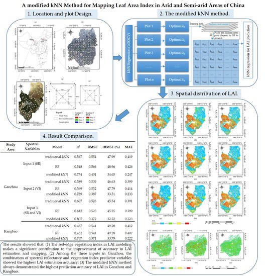
Study Area	Spectral Variables	Model	R2	RMSE	rRMSE (%)	MAE
Ganzhou		traditional kNN	0.567	0.554	47.99	0.419
	Input 1 (SR)	RF	0.548	0.566	48.96	0.426
		modified kNN	0.774	0.401	34.65	0.247
		traditional kNN	0.589	0.539	46.63	0.399
	Input 2 (VI)	RF	0.569	0.552	47.79	0.414
		modified kNN	0.789	0.387	33.51	0.233
		traditional kNN	0.607	0.526	45.54	0.391
	Input 3 (SR and VI)	RF	0.612	0.523	45.25	0.399
		modified kNN	0.807	0.372	32.22	0.223
Kangbao		traditional kNN	0.467	0.541	49.20	0.412
	Eight selected spectral variables	RF	0.452	0.541	49.28	0.407
		modified kNN	0.767	0.371	33.79	0.222

). The estimation effectiveness of the modified kNN is significantly better than the other two models based on the significant difference test of absolute residuals between the estimated and observed LAI values among the models for each of the set inputs of the selected spectral variables using the student_T distribution (

Table A3. The test values (p-values) of significant differences among the models for each of the input sets of spectral variables based on the absolute residuals between the estimated and observed LAI values using the student_T distribution in Ganzhou and Kangbao.

	Inputs (Spectral Variables)	Model	Traditional kNN	RF
Ganzhou	Input 1 (bands)	Traditional kNN
		RF	−0.819 (0.413)
		modified kNN	23.625 (0)	22.295 (0)
	Input 2 (VIs)	Traditional kNN
		RF	−1.759 (0.079)
		modified kNN	21.448 (0)	19.668 (0)
	Input 3 (bands and VIs)	Traditional kNN
		RF	−0.963 (0.336)
		modified kNN	21.120 (0)	19.106 (0)
Kangbao	Eight selected spectral variables	Traditional kNN
		RF	0.271 (0.787)
		modified kNN	10.709 (0)	9.911 (0)

in Appendix A). The RF slightly outperformed the traditional kNN for the set input 1 and input 3 of the selected spectral variables (Table 4); however, their RMSE values are very similar and there is no significant difference of absolute residuals (Table A3 in Appendix A). For the set input 2, the RMSE value from the traditional kNN is slightly lower than that obtained by RF and the difference between their absolute residuals is not significant. The global k values of the traditional kNN for all three set inputs are 17, 12, and 33, respectively. Using the local optimal k values in the modified kNN significantly improved the prediction accuracy compared with the traditional kNN and RF, regardless of the three set inputs of the selected spectral variables.

In Kangbao County, the modified kNN has the highest R² and the smallest values of RMSE, rRMSE, and MAE (Table 4). The modified kNN demonstrates a reduction of RMSE by 31.4% compared with both the traditional kNN and RF. The global k value obtained using the traditional kNN is 8. There is no significant difference of the absolute residuals between the traditional kNN and RF; however, the modified kNN resulted in a significantly more accurate prediction of LAI than the other two methods (Table A3 in Appendix A).

The spatial distributions of LAI predictions obtained by the traditional kNN, RF, and modified kNN using the three set inputs of the selected predictors generally look similar over the study area of Ganzhou (Figure 4). Most of the larger LAI predictions are distributed in the central and western regions, while the predicted values in the southern and southwest regions are relatively smaller. The smallest LAI values are found in the northern part of the region. The spatial patterns of LAI are basically consistent with the actual LAI distribution in the study area. Moreover, most of the smaller predicted LAI values in Kangbao County are noticed in the northern part (Figure 5). The greater predicted values of LAI are mainly distributed in the central and western regions. The modified kNN led to more reasonable spatial distributions than the tradition kNN and RF based on those of the LAI measurements in both study areas.

Figure 6 and Figure 7 show the LAI values predicted by three models versus the observed values. There are overestimations and underestimations found for some of the sample plots for all of the models and all of the set inputs of the selected spectral variables in Ganzhou District (Figure 6). Given the same model, compared with those from the set input 1 and input 2, the overestimations and underestimations were decreased by using the set input 3. On the other hand, given the same set input, the modified kNN greatly reduced the overestimations and underestimations compared with the traditional kNN and RF. The residuals from the modified kNN tended to be randomly distributed. For Kangbao County, the traditional kNN and RF led to obvious overestimations and underestimations (Figure 7). The values of the overestimations and underestimations were greatly reduced by the modified kNN.

3.3. Uncertainty Analysis

In order to evaluate the adaptation of the modified kNN, the following uncertainty analyses of estimates from the modified kNN were conducted: (1) significance test of correlation between the residuals and the predictions of LAI; (2) significance test of correlation between the residuals and the spectral variables; and (3) spatial autocorrelation analysis of the residuals.

In both Ganzhou and Kangbao, there are negative correlations between the residuals and predicted LAI values (

Table 5. The Pearson correlation coefficients of the residuals with the predicted LAI and the spectral variables used by the modified kNN in Ganzhou and Kangbao (Note: * at the significance level of 0.05, and ** at the significance level of 0.01).

Study Area	Factors	Residual	Factors	Residual
Ganzhou	30 m × 30 m spatial resolution		1000 m × 1000 m spatial resolution
	Predicted LAI	−0.114*	Predicted LAI	−0.239*
	ARVI	0.038	B2	0.063
	B2	−0.074	NDVI	−0.081
	B11	−0.035
	RECI	0.078
Kangbao	Predicted LAI	−0.295**
	B7	0.163
	NDVI	−0.135
	B6	0.181*
	ARVI	0.208*
	B4	0.114
	B3	0.113
	B1	0.122
	B2	0.120

) and the correlation coefficients are statistically significantly different from zero at the significance level of 0.05. This implies that the residuals decrease as the predictions of LAI increase. Moreover, there are no significant correlations between the residuals and the four spectral variables used in Ganzhou, indicating that the predictors have no significant effects on the uncertainty measure of the estimates (Table 5). For Kangbao County, out of the eight predictors used, only Band 6 and the ARVI are significantly correlated with the residuals. This means that the residuals as uncertainties of LAI predictions are significantly affected by Band 6 and the ARVI, but not others.

The results of Moran’s I show that at the 30 m spatial resolution, the spatial autocorrelation of residuals for the LAI predictions using the modified kNN is significant at the significance level of 0.05 in Ganzhou, but not in Kangbao County. This means that in Ganzhou, overall, the residuals are spatially clustered with high or low values, while in Kangbao, the residuals are randomly distributed over the space. To identify what caused the spatial clustering of the residuals, the Sentinel-2 image was scaled up from the spatial resolution of 30 m × 30 m to 1000 m × 1000 m to match the data from the sample blocks using the cubic convolution method and the modified kNN was then utilized with Band 2 and the NDVI selected to map LAI. The results show that the obtained R², RMSE, rRMSE, and MAE are 0.827, 0.364, 32.85%, and 0.209, respectively. The residuals are significantly correlated with the predicted LAI values, but not with the two spectral variables used at the significance level of 0.05 (Table 5). More importantly, the spatial autocorrelation of the residuals is not significant (

Table 6. Spatial autocorrelation statistical results of the residuals obtained from modified kNN in Ganzhou and Kangbao.

Study Area	Parameter	Value
	30 m × 30 m spatial resolution
	Moran I	0.237
	Variance	0.001
	Z	6.576
Ganzhou	p	0.000
	1000 m × 1000 m spatial resolution
	Moran I	0.079
	Variance	0.005
	Z	1.249
	p	0.211
Kangbao	30 m × 30 m spatial resolution
	Moran I	0.018
	Variance	0.004
	Z	0.384
	p	0.700

). This implies that the spatial autocorrelation of the residuals at the 30 m spatial resolution was caused by the five nested sample plots within each of the 1000 m × 1000 m sample blocks in Ganzhou.

4. Discussion

4.1. Spectral Variable Selection for LAI Mapping

This study demonstrated that the combination of the original spectral bands with the VIs derived from the red-edge bands of the Sentinel-2 image in Ganzhou was more accurate and effective in predicting the LAI of arid and semi-arid areas than separate sets of the original bands and the VIs. The red-edge band-derived VIs were consistently selected as the most important predictors by RF. The accuracy of LAI prediction using the modified kNN based on the combination (input 3) of the original bands and VIs was markedly improved. The results showed that using the set input 3 reduced the RMSE by 5.1%, 7.6%, and 7.2% compared with the set input 1, and by 2.4%, 5.3%, and 3.9% compared with the set input 2, based on the traditional kNN, RF, and modified kNN, respectively. This implied that regardless of the non-parametric models, using the set input 3 of the spectral variables provided more accurate predictions of LAI. The RF enables the spectral variables to be ranked in accordance with their importance based on their contributions to decreasing the RMSE [59] and then selects the spectral variables that significantly improved the predictions of LAI. Moreover, non-parametric methods do not require an assumption about the normal distribution of predictors and also do not need to consider the collinearity between the spectral variables [29,30,31].

Appropriately selecting spectral variables to parameterize models can significantly improve the prediction accuracy and mapping effectiveness of models. Spectral reflectance bands are directly related to the characteristics of the vegetation canopy on the ground and can be used as basic predictors for modeling [59]. The VIs that are derived from the spectral reflectance bands can effectively reveal the growth and health characteristics of vegetation [65]. For example, the enhanced vegetation index (EVI) is sensitive to dense vegetation, and can quickly respond to changes in the canopy structure and chlorophyll content [66], while NDVI is sensitive to the changes in LAI during plant growth, but not to the multi-layer vegetation canopy structure. VIs based on the red-edge bands (such as RENDVI, RESR, and RECI) can partially overcome the saturation of traditional Vis, such as NDVI [67], and improve the LAI prediction accuracy. In addition, the red-edge bands can respond to minor changes in spectral reflectance and LAI [2]. However, in arid and semi-arid regions, large bare land areas can produce a high intensity and wide bandwidth of reflectance that masks vegetation as most of the vegetation is represented in gray or green colors with signals that are too weak to be captured by sensors. Some VSs obtained by combining different bands can detect vegetation growth by highlighting or emphasizing band information, but they also weaken the information of other ground objects. For Ganzhou, the original spectral bands, VIs, and their combination were used to screen the performance of prediction models. It was found that there were differences in the prediction effectiveness when either the spectral bands or VIs alone were used as predictors. The VIs performed better than the original spectral bands, while the combination of spectral bands and VIs performed the best. This confirmed the findings of previous literature [12,47,52,53]. Integrating the spectral bands and VIs can greatly reduce the error of LAI estimation in arid and semi-arid areas, but there is no evidence to show that the combination can completely eliminate the impact of spectral saturation in densely vegetated areas.

4.2. Comparison of LAI Prediction Models

Arid and semi-arid areas are characterized by ecosystems consisting of complex plant communities. As a result, the relationship between LAI and spectral variables is complex and often non-linear, and cannot be accounted for by a simple linear relationship. Non-parametric models allow one to ignore the collinearity between spectral variables and make it more appropriate to utilize them for mapping LAI in arid and semi-arid areas. The methods also allow combinations of predictors that have different characteristics and thus provide the potential to improve the estimation of LAI in arid and semi-arid areas.

As typical non-parametric methods, RF and kNN have been widely used for predicting vegetation parameters with various types of remote sensing data. The RF can determine the importance of feature variables and build a large number of regression trees for prediction [28]. The kNN does not require the training or estimation of model parameters. In this study, the traditional kNN and RF methods led to similar RMSE values of LAI predictions, with the range of 0.539–0.566 m²/m², regardless of the three set inputs of the spectral variables in Ganzhou. The results are consistent with previous findings [12,52]. For example, Zhu et al. [12] obtained the RMSE of 0.45 for the estimation of Mangrove LAI using RF regression and the spectral variables from a WorldView-2 satellite image and red-edge bands-derived VIs. Delegido et al. [52] used Sentinel-2 red-edge bands for LAI mapping by applying RTM models and obtained an RMSE of 0.57.

The k value, indicating the number of nearest neighbors, plays an important role in improving the estimation accuracy for the traditional kNN. The k value often differs from place to place in the LAI estimation of arid and semi-arid areas with diverse vegetation canopy structures. The complex topographic features are also considered to be important factors that affect the k value [32]. Tokola et al. [33] suggested the range of k values from 10 to 15 when forest parameters were estimated using the traditional kNN, while Tomppo et al. [34] pointed out that k values between 5 and 10 led to accurate results in the Finnish multi-source national forest inventory. Moeur and Stage [35] even implied the use of one nearest plot for the k value to maintain the variation of the original data. However, due to spatial variability and heterogeneity, using the same k value globally usually limits the prediction accuracy of the kNN. Therefore, in this study, the modified kNN was developed by integrating the traditional kNN with RF for mapping LAI in arid and semi-arid areas of China. Using RF and the traditional kNN alone showed significantly lower accuracies in LAI prediction compared with the modified kNN, which exploited an optimal k for each pixel. For all of the set inputs of the selected spectral variables, the modified kNN decreased the RMSE of the LAI predictions by 27.6% to 29.3% and 28.9% to 29.9% compared with the traditional kNN and RF, respectively, in Ganzhou. The corresponding decrease of the RMSE value was 31.4% for both of the compared methods in Kangbao. The modified kNN thus performed significantly better than the traditional kNN and RF alone.

Each of the non-parametric models possesses its own unique advantages and disadvantages. For example, it is not possible for the kNN method to make predictions beyond the data [32]. However, the kNN method does not need to be trained in advance and does not require normal distributions of data, whereas RF provides the importance rank of all predictors used in the prediction, which is of great significance for the rapid and accurate selection of predictors. The problem of high-dimensional data can be overcome by both methods [23]. However, when RF is used, the estimation accuracy of LAI is, to a great extent, limited by the sample size. A too small sample size often leads to smoothing of the spatial distribution of LAI by RF. In addition, the use of a global k value in the traditional kNN impedes the improvement of the LAI estimation accuracy. This is especially true in complex landscapes that are characterized by a great spatial variability and heterogeneity of the vegetation canopy structure. On the other hand, the traditional kNN can be improved by determining an optimal k value for each pixel. However, for a location to be estimated, its optimal k value is unknown. Sun et al. [27] proposed a method to search for the optimal k value for each unknown location based on the stable change rate of estimation variance for mapping the percentage vegetation cover in arid and semi-arid areas using Landsat images.

Using hybrid methods enables one to take advantage of the models and improve the prediction accuracy. The key issue is how to combine the models and make full use of their advantages. In this study, the traditional kNN and RF were integrated to develop the modified kNN for generating the spatial distribution of LAI. In the integrated method, the traditional kNN was utilized to derive the optimal k values for the sampled locations and RF was then used to conduct image classification of the landscape and extrapolate the optimal k values from the sampled locations to the unknown locations. The modified kNN showed more promise for improving the estimation accuracy of LAI compared with the traditional RF and kNN. Compared with the one in the study of Sun et al. [27], theoretically, the modified kNN proposed in this study should provide more accurate k values and thus more accurate estimates of LAI, because it uses the RMSE instead of the variance of k nearest plots. In fact, in this study, a comparison of the modified kNN based on the RMSE with the one based on variance by Sun et al. [27] was implemented. It was found that in Ganzhou, the variance-based modified kNN resulted in the rRMSE values of 47.87%, 46.28%, and 44.93% for the variable set input 1, input 2, and input 3, respectively, which were only slightly smaller than those obtained by the traditional kNN, but significantly greater than those obtained by the RMSE-based modified kNN in this study. A similar conclusion was achieved in Kangbao.

4.3. Limitations and Suggestions for Further Improvement

Many factors can influence the accuracy of mapping biophysical vegetation parameters such as LAI. The factors include the selection of different sensors with spectral and radiometric characteristics, sample sizes, and sampling strategies; vegetation cover types; and the modeling methods to be applied. Moreover, validation of the final estimates can be influenced by the instruments and procedures used for the acquisition of reference data. The contribution of uncertainty from each of the components to the residuals of predictions may vary from case to case. How the uncertainties affect the estimation accuracy of biophysical vegetation parameters is unknown.

In this study, a comprehensive error and uncertainty budget was not calculated due to limited space and time. Instead, the characteristics of the residuals for the LAI predictions using the proposed kNN and the effects of the selected predictors on the residuals were analyzed. It was found that the residuals were negatively and significantly correlated with the LAI predictions in both Ganzhou and Kangbao. This implies that the smaller the LAI predictions, the greater the relative uncertainties. This is mainly because of the sparsely vegetated areas in which mixed pixels widely exist and the spectral reflectance from the bare soil areas as noise might have significantly impacted the signals of the vegetation canopies. Moreover, in Ganzhou, all of the selected spectral variables did not have significant effects on the residuals, while out of the eight selected predictors in Kangbao, the weakly significant influence only came from band 6 and ARVI, with the correlation coefficients of 0.181 and 0.208 being slightly greater than the critical value of 0.178 at the significance level of 0.05. In addition, in Ganzhhou, the residuals were spatially clustered at the spatial resolution of 30 m × 30 m, but not at the spatial resolution of 1000 m × 1000 m, mainly due to five 30 m × 30 m sample plots being nested within each of the 1000 m × 1000 m sample blocks. There was also no spatial autocorrelation of the residuals in Kangbao because the sample blocks were not used and all of the sample plots were systematically allocated across the study area. This implies that taking into account the spatial autocorrelation in the proposed kNN may lead to a further improvement of LAI estimation.

There are other specific limitations when mapping LAI in arid and semi-arid areas using non-parametric methods. The arid and semi-arid areas are often remote, large, and sparsely vegetated and populated. Selecting the most appropriate remote sensing images should be critical. MODIS products with free downloading available, large coverages, and fine temporal resolutions provide the potential to quickly monitor the dynamics of LAI in arid and semi-arid areas, but their coarse spatial resolutions will lead to a great number of mixed pixels, which will degrade the quality of LAI products. High spatial resolution and hyperspectral images may greatly reduce the number of mixed pixels, but a high cost is required to get the images to cover large arid and semi-arid areas. This is the major reason why Sentinel-2 and Landsat 8 OLI images for Ganzhou and Kangbao, respectively, with free downloading and a medium spatial resolution, were chosen in this study.

Due to the spatial variability and heterogeneity of LAI in arid and semi-arid areas, the sampling strategy is very important when capturing the characteristics of the canopy structure at both a global and local level. In this study, a stratified random sampling method with the number of 30 m × 30 m sample plots for each land type proportional to the corresponding area was employed. Within each plot, five sub-plots of 1 m × 1 m were allocated to measure LAI and the average LAI was then taken as the value of the whole plot. This greatly reduced the cost of collecting LAI observations in the field. In fact, it was impossible to make thorough measurements of each plot. Using the average of five 1 m × 1 m sub-plot LAI values can reduce the uncertainty caused by spatial heterogeneity [2].

5. Conclusions

Predicting and mapping LAI in arid and semi-arid regions is essential for the assessment of regional and global land degradation and desertification. Non-parametric methods, such as kNN and RF, can effectively combine remote sensing images and sample plot data to map LAI. However, in arid and semi-arid areas, the accuracy of these models is limited because of shortcomings that exist in the methods, remote and large areas, and the characteristics of sparsely vegetated and populated areas. In this study, the modified kNN method was proposed by integrating the traditional kNN and RF to map LAI in Ganzhou District and Kangbao County using Sentinel-2 and Landsat 8 images, respectively, with sample plot data. The locally optimal k values of kNN were assessed based on the RMSE. In Ganzhou District, three sets of input predictors, including (1) spectral reflectance bands, (2) Vis, and (3) the combination of bands and VIs, were used to compare the modified kNN with the traditional kNN and RF. It was found that (1) the red-edge bands of the Sentinel-2 image had a high correlation with LAI, and the red-edge band-derived VIs made significant contributions to the improvement of accuracy in mapping LAI; (2) among the three sets of predictors, the combination of spectral bands and VIs showed the highest LAI estimation accuracy, regardless of the RF, traditional kNN, and modified kNN; and (3) the modified kNN demonstrated the highest prediction accuracy of LAI in the study area for all three sets of predictors. Compared with the traditional kNN and RF, the modified kNN reduced the rRMSE by 27.8% and 29.2% for the set input 1 of predictors, 28.1% and 29.9% for the set input 2, and 29.2% and 28.8% for the set input 3 in Ganzhou, respectively. In Kangbao, the corresponding decrease of rRMSE by the modified kNN was 31.4% for both of the compared models. The proposed kNN was thus shown to be very promising for improving the estimation and mapping of LAI in arid and semi-arid areas.

References

- Neinavaz, E.; Darvishzadeh, R.; Skidmore, A.K.; Abdullah, H. Integration of Landsat-8 Thermal and Visible-Short Wave Infrared Data for Improving Prediction Accuracy of Forest Leaf Area Index. Remote Sens. 2019, 11, 390. [Google Scholar] [CrossRef] [Green Version]
- Qiao, K.; Zhu, W.; Xie, Z.; Li, P. Estimating the Seasonal Dynamics of the Leaf Area Index Using Piecewise LAI-VI Relationships Based on Phenophases. Remote Sens. 2019, 11, 689. [Google Scholar] [CrossRef] [Green Version]
- Fan, W.; Liu, Y.; Xu, X.; Chen, G.; Zhang, B. A new FAPAR analytical model based on the law of energy conservation: A case study in China. IEEE J. Sel. Top. Appl. Earth Obs. Remote Sens. 2014, 7, 3945–3955. [Google Scholar] [CrossRef]
- Tian, Y.; Zheng, Y.; Zheng, C.; Xiao, H.; Fan, W.; Zou, S.; Wu, B.; Yao, Y.; Zhang, A.; Liu, J. Exploring scale-dependent ecohydrological responses in a large endorheic river basin through integrated surface water-groundwater modeling. Water Resour. Res. 2015, 51, 4065–4085. [Google Scholar] [CrossRef]
- Potithep, S.; Nagai, S.; Nasahara, K.N.; Muraoka, H.; Suzuki, R. Two separate periods of the LAI–VIs relationships using in situ measurements in a deciduous broadleaf forest. Agric. For. Meteorol. 2013, 169, 148–155. [Google Scholar] [CrossRef]
- Simic, A.; Fernandes, R.; Wang, S. Assessing the impact of leaf area index on evapotranspiration and groundwater recharge across a shallow water region for diverse land cover and soil properties. J. Water Resour. Hydraul. Eng. 2014, 3, 60–73. [Google Scholar]
- Verrelst, J.; Rivera, J.P.; Veroustraete, F.; Muñoz-Marí, J.; Clevers, J.G.; Camps-Valls, G.; Moreno, J. Experimental Sentinel-2 LAI estimation using parametric, non-parametric and physical retrieval methods–A comparison. ISPRS J. Photogramm. Remote Sens. 2015, 108, 260–272. [Google Scholar]
- Upreti, D.; Huang, W.; Kong, W.; Pascucci, S.; Pignatti, S.; Zhou, X.; Ye, H.; Casa, R. A Comparison of Hybrid Machine Learning Algorithms for the Retrieval of Wheat Biophysical Variables from Sentinel-2. Remote Sens. 2019, 11, 481. [Google Scholar] [CrossRef] [Green Version]
- Wei, C.; Huang, J.; Mansaray, L.R.; Li, Z.; Liu, W.; Han, J. Estimation and Mapping of Winter Oilseed Rape LAI from High Spatial Resolution Satellite Data Based on a Hybrid Method. Remote Sens. 2017, 9, 488. [Google Scholar] [CrossRef] [Green Version]
- Su, W.; Huang, J.; Liu, D.; Zhang, M. Retrieving Corn Canopy Leaf Area Index from Multitemporal Landsat Imagery and Terrestrial LiDAR Data. Remote Sens. 2019, 11, 572. [Google Scholar] [CrossRef] [Green Version]
- Zhou, H.; Wang, J.; Liang, S.; Xiao, Z. Extended Data-Based Mechanistic Method for Improving Leaf Area Index Time Series Estimation with Satellite Data. Remote Sens. 2017, 9, 533. [Google Scholar] [CrossRef] [Green Version]
- Zhu, Y.; Liu, K.; Liu, L.; Myint, S.W.; Wang, S.; Liu, H.; He, Z. Exploring the Potential of WorldView-2 Red-Edge Band-Based Vegetation Indices for Estimation of Mangrove Leaf Area Index with Machine Learning Algorithms. Remote Sens. 2017, 9, 1060. [Google Scholar] [CrossRef] [Green Version]
- Zhao, J.; Li, J.; Liu, Q.; Wang, H.; Chen, C.; Xu, B.; Wu, S. Comparative Analysis of Chinese HJ-1 CCD, GF-1 WFV and ZY-3 MUX Sensor Data for Leaf Area Index Estimations for Maize. Remote Sens. 2018, 10, 68. [Google Scholar] [CrossRef] [Green Version]
- Yin, G.; Li, J.; Liu, Q.; Fan, W.; Xu, B.; Zeng, Y.; Zhao, J. Regional Leaf Area Index Retrieval Based on Remote Sensing: The Role of Radiative Transfer Model Selection. Remote Sens. 2015, 7, 4604–4625. [Google Scholar] [CrossRef] [Green Version]
- Feret, J.-B.; François, C.; Asner, G.P.; Gitelson, A.A.; Martin, R.E.; Bidel, L.P.; Ustin, S.L.; Le Maire, G.; Jacquemoud, S. PROSPECT-4 and 5: Advances in the leaf optical properties model separating photosynthetic pigments. Remote Sens. Environ. 2008, 112, 3030–3043. [Google Scholar] [CrossRef]
- Jacquemoud, S.; Verhoef, W.; Baret, F.; Bacour, C.; Zarco-Tejada, P.J.; Asner, G.P.; François, C.; Ustin, S.L. PROSPECT+ SAIL models: A review of use for vegetation characterization. Remote Sens. Environ. 2009, 113, S56–S66. [Google Scholar] [CrossRef]
- Verhoef, W. Light scattering by leaf layers with application to canopy reflectance modeling: The SAIL model. Remote Sens. Environ. 1984, 16, 125–141. [Google Scholar] [CrossRef] [Green Version]
- Si, Y.; Schlerf, M.; Zurita-Milla, R.; Skidmore, A.; Wang, T. Mapping spatio-temporal variation of grassland quantity and quality using MERIS data and the PROSAIL model. Remote Sens. Environ. 2012, 121, 415–425. [Google Scholar] [CrossRef]
- Le Maire, G.; Marsden, C.; Verhoef, W.; Ponzoni, F.J.; Seen, D.L.; Bégué, A.; Stape, J.-L.; Nouvellon, Y. Leaf area index estimation with MODIS reflectance time series and model estimation during full rotations of Eucalyptus plantations. Remote Sens. Environ. 2011, 115, 586–599. [Google Scholar] [CrossRef]
- Liang, L.; Qin, Z.; Zhao, S.; Di, L.; Zhang, C.; Deng, M.; Lin, H.; Zhang, L.; Wang, L.; Liu, Z. Estimating crop chlorophyll content with hyperspectral vegetation indices and the hybrid estimation method. Int. J. Remote Sens. 2016, 37, 2923–2949. [Google Scholar] [CrossRef]
- Atzberger, C. Object-based retrieval of biophysical canopy variables using artificial neural nets and radiative transfer models. Remote Sens. Environ. 2004, 93, 53–67. [Google Scholar] [CrossRef]
- García-Gutiérrez, J.; Martínez-álvarez, F.; Troncoso, A.; Riquelme, J.C. A comparison of machine learning regression techniques for lidar-derived estimation of forest variables. Neurocomputing 2015, 167, 24–31. [Google Scholar] [CrossRef]
- Yuan, H.; Yang, G.; Li, C.; Wang, Y.; Liu, J.; Yu, H.; Feng, H.; Xu, B.; Zhao, X.; Yang, X. Retrieving Soybean Leaf Area Index from Unmanned Aerial Vehicle Hyperspectral Remote Sensing: Analysis of RF, ANN, and SVM Regression Models. Remote Sens. 2017, 9, 309. [Google Scholar] [CrossRef] [Green Version]
- Yun, T.; An, F.; Li, W.; Sun, Y.; Cao, L.; Xue, L. A Novel Approach for Retrieving Tree Leaf Area from Ground-Based LiDAR. Remote Sens. 2016, 8, 942. [Google Scholar] [CrossRef] [Green Version]
- Li, Z.; Wang, J.; Tang, H.; Huang, C.; Yang, F.; Chen, B.; Wang, X.; Xin, X.; Ge, Y. Predicting Grassland Leaf Area Index in the Meadow Steppes of Northern China: A Comparative Study of Regression Approaches and Hybrid Geostatistical Methods. Remote Sens. 2016, 8, 632. [Google Scholar] [CrossRef] [Green Version]
- Cong, X.; Bruce, M.; Justin, M. Evaluation of modelling approaches in predicting forest volume and stand age for small-scale plantation forests in new zealand with rapideye and lidar. Int. J. Appl. Earth Obs. Geoinf. 2018, 73, 386–396. [Google Scholar]
- Sun, H.; Wang, Q.; Wang, G.; Lin, H.; Luo, P.; Li, J.; Zeng, S.; Xu, X.; Ren, L. Optimizing kNN for Mapping Vegetation Cover of Arid and Semi-Arid Areas Using Landsat Images. Remote Sens. 2018, 10, 1248. [Google Scholar] [CrossRef] [Green Version]
- Breiman, L. Random Forests. Mach. Learn. 2001, 45, 5–32. [Google Scholar] [CrossRef] [Green Version]
- Ismail, R.; Mutanga, O.; Kumar, L. Modeling the potential distribution of pine forests susceptible to SirexNoctilio infestations in Mpumalanga, South Africa. Trans. GIS 2010, 14, 709–726. [Google Scholar] [CrossRef]
- Vincenzi, S.; Zucchetta, M.; Franzoi, P.; Pellizzato, M.; Pranovi, F.; De Leo, G.A.; Torricelli, P. Application of a Random Forest algorithm to predict spatial distribution of the potential yield of Ruditapes Philippinarum in the Venice lagoon, (Italy). Ecol. Model. 2011, 222, 1471–1478. [Google Scholar] [CrossRef]
- Chen, Y.; Li, L.; Lu, D.; Li, D. Exploring Bamboo Forest Aboveground Biomass Estimation Using Sentinel-2 Data. Remote Sens. 2019, 11, 7. [Google Scholar] [CrossRef] [Green Version]
- Katila, M.; Tomppo, E. Selecting Estimation Parameters for the Finnish Multisource National Forest Inventory. Remote Sens. Environ. 2001, 76, 16–32. [Google Scholar] [CrossRef]
- Tokola, T.; PitkaÈnen, J.; Partinen, S.; Muinonen, E. Point accuracy of a non-parametric method in estimation of forest characteristics with different satellite materials. Int. J. Remote Sens. 1996, 17, 2333–2351. [Google Scholar] [CrossRef]
- Tomppo, E.; Haakana, M.; Katila, M. Multi-Source National Forest Inventory–Methods and Applications. Efi Proc. 1996, 7, 16–32. [Google Scholar]
- Moeur, M.; Stage, A.R. Most similar neighbor: An improved sampling inference procedure for natural resource planning. For. Sci. 1995, 41, 337–359. [Google Scholar]
- McRoberts, R.E.; Nelson, M.D.; Wendt, D.G. Stratified estimation of forest area using satellite imagery, inventory data, and the k-Nearest Neighbors technique. Remote Sens. Environ. 2002, 82, 457–468. [Google Scholar] [CrossRef]
- Thessler, S.; Sesnie, S.; Bendaña, Z.S.R.; Ruokolainen, K.; Tomppo, E.; Finegan, B. Using k-nn and discriminant analyses to classify rain forest types in a Landsat TM image over northern (Costa Rica). Remote Sens. Environ. 2008, 112, 2485–2494. [Google Scholar] [CrossRef]
- Tan, K.; Hu, J.; Li, J.; Du, P. A novel semi-supervised hyperspectral image classification approach based on spatial neighborhood information and classifier combination. ISPRS J. Photogramm. Remote Sens. 2015, 105, 19–29. [Google Scholar] [CrossRef]
- Tomppo, E.O.; Gagliano, C.; De Natale, F.; Katila, M.; McRoberts, R.E. Predicting categorical forest variables using an improved k-Nearest Neighbour estimator and Landsat imagery. Remote Sens. Environ. 2009, 113, 500–517. [Google Scholar] [CrossRef]
- McRoberts, R.E.; Magnussen, S.; Tomppo, E.O.; Chirici, G. Parametric, bootstrap, and jackknife variance estimators for the k-Nearest Neighbors technique with illustrations using forest inventory and satellite image data. Remote Sens. Environ. 2011, 115, 3165–3174. [Google Scholar] [CrossRef]
- Tomppo, E.; Olsson, H.; Ståhl, G.; Nilsson, M.; Hagner, O.; Katila, M. Combining national forest inventory field plots and remote sensing data for forest databases. Remote Sens. Environ. 2008, 112, 1982–1999. [Google Scholar] [CrossRef]
- Franco–Lopez, H.; Ek, A.R.; Bauer, M.E. Estimation and mapping of forest stand density, volume, and cover type using the k-nearest neighbors method. Remote Sens. Environ. 2001, 77, 251–274. [Google Scholar] [CrossRef]
- Labrecque, S.; Fournier, R.A.; Luther, J.E.; Piercey, D. A comparison of four methods to map biomass from Landsat-TM and inventory data in western Newfoundland. For. Ecol. Manag. 2006, 226, 129–144. [Google Scholar] [CrossRef]
- Fuchs, H.; Magdon, P.; Kleinn, C.; Flessa, H. Estimating aboveground carbon in a catchment of the Siberian forest tundra: Combining satellite imagery and field inventory. Remote Sens. Environ. 2009, 113, 518–531. [Google Scholar] [CrossRef]
- Tomppo, E.; Halme, M. Using coarse scale forest variables as ancillary information and weighting of variables in k-NN estimation: A genetic algorithm approach. Remote Sens. Environ. 2004, 92, 1–20. [Google Scholar] [CrossRef]
- McRoberts, R.E.; Næsset, E.; Gobakken, T. Optimizing the k-Nearest Neighbors technique for estimating forest aboveground biomass using airborne laser scanning data. Remote Sens. Environ. 2015, 163, 13–22. [Google Scholar] [CrossRef]
- Zhu, J.; Huang, Z.; Sun, H.; Wang, G. Mapping Forest Ecosystem Biomass Density for Xiangjiang River Basin by Combining Plot and Remote Sensing Data and Comparing Spatial Extrapolation Methods. Remote Sens. 2017, 9, 241. [Google Scholar] [CrossRef] [Green Version]
- Mura, M.; McRoberts, R.E.; Chirici, G.; Marchetti, M. Statistical inference for forest structural diversity indices using airborne laser scanning data and the k-Nearest Neighbors technique. Remote Sens. Environ. 2016, 186, 678–686. [Google Scholar] [CrossRef]
- Hall, P.; Park, B.U.; Samworth, R.J. Choice of neighbor order in nearest-neighbor classification. Ann. Stat. 2008, 36, 2135–2152. [Google Scholar] [CrossRef]
- James, G.; Witten, D.; Hastie, T.; Tibshirani, R. Introduction to Statistical Learning: With Applications in R; Springer: New York, NY, USA, 2017. [Google Scholar]
- Lin, C.; Thomson, G.; Popescu, S. An IPCC-Compliant Technique for Forest Carbon Stock Assessment Using Airborne LiDAR-Derived Tree Metrics and Competition Index. Remote Sens. 2016, 8, 528. [Google Scholar] [CrossRef] [Green Version]
- Delegido, J.; Verrelst, J.; Alonso, L.; Moreno, J. Evaluation of Sentinel-2 Red-Edge Bands for Empirical Estimation of Green LAI and Chlorophyll Content. Sensors 2011, 11, 7063–7081. [Google Scholar] [CrossRef] [PubMed] [Green Version]
- Vuolo, F.; Żółtak, M.; Pipitone, C.; Zappa, L.; Wenng, H.; Immitzer, M.; Weiss, M.; Baret, F.; Atzberger, C. Data Service Platform for Sentinel-2 Surface Reflectance and Value-Added Products: System Use and Examples. Remote Sens. 2016, 8, 938. [Google Scholar] [CrossRef] [Green Version]
- Tang, X.; Fehrmann, L.; Guan, F.; Forrester, D.I.; Guisasola, R.; Kleinn, C. Inventory-based estimation of forest biomass in Shitai County, China: A comparison of five methods. Ann. For. Res. 2016, 59, 269–280. [Google Scholar] [CrossRef] [Green Version]
- Li, Y.; Li, C.; Li, M.; Liu, Z. Influence of Variable Selection and Forest Type on Forest Aboveground Biomass Estimation Using Machine Learning Algorithms. Forests 2019, 10, 1073. [Google Scholar] [CrossRef] [Green Version]
- Chen, J.M.; Cihlar, J. Retrieving leaf area index of boreal conifer forests using landsat tm images. Remote Sens. Environ. 1996, 55, 153–162. [Google Scholar] [CrossRef]
- Piayda, A.; Dubbert, M.; Werner, C.; Vaz Correia, A.; Pereira, J.S.; Cuntz, M. Influence of woody tissue and leaf clumping on vertically resolved leaf area index and angular gap probability estimates. For. Ecol. Manag. 2015, 340, 103–113. [Google Scholar] [CrossRef]
- Dong, T.; Liu, J.; Shang, J.; Qian, B.; Ma, B.; Kovacs, J.M.; Shi, Y. Assessment of red-edge vegetation indices for crop leaf area index estimation. Remote Sens. Environ. 2019, 222, 133–143. [Google Scholar] [CrossRef]
- Lu, D.; Chen, Q.; Wang, G.; Liu, L.; Li, G.; Moran, E. A survey of remote sensing–based aboveground biomass estimation methods in forest ecosystems. Int. J. Earth. 2016, 9, 63–105. [Google Scholar] [CrossRef]
- Crookston, N.L.; Finley, A.O. yaImpute: An R Package for k NN Imputation. J. Stat. Soft. 2008, 23. [Google Scholar]
- Finley, A.O.; McRoberts, R.E. Efficient k-nearest neighbor searches for multi-source forest attribute mapping. Remote Sens. Environ. 2008, 112, 2203–2211. [Google Scholar] [CrossRef]
- Gjertsen, A.K. Accuracy of forest mapping based on Landsat TM data and a kNN-based method. Remote Sens. Environ. 2007, 110, 420–430. [Google Scholar] [CrossRef]
- Pal, M. Random forest classifier for remote sensing classification. Int. J. Remote Sens. 2005, 26, 217–222. [Google Scholar] [CrossRef]
- Willmott, C.J.; Ackleson, S.G.; Davis, R.E.; Feddema, J.J.; Klink, K.M.; Legates, D.R. Statistics for the evaluation and comparison of models. J. Geophys. Res. 1985, 90, 8995. [Google Scholar] [CrossRef] [Green Version]
- Sims, D.; Gamon, J. Relationships between leaf pigment content and spectral reflectance across a wide range of species, leaf structures and developmental stages. Remote Sens. Environ. 2002, 81, 337–354. [Google Scholar] [CrossRef]
- Gitelson, A.A.; Viña, A.; Arkebauer, T.J.; Rundquist, D.C.; Keydan, G.; Leavitt, B. Remote estimation of leaf area index and green leaf biomass in maize canopies. Geophys. Res. Lett. 2003, 30, 1248. [Google Scholar] [CrossRef] [Green Version]
- Yang, W.; Huang, D.; Tan, B.; Stroeve, J.C.; Shabanov, N.V.; Knyazikhin, Y.; Nemani, R.R.; Myneni, R.B. Analysis of leaf area index and fraction of PAR absorbed by vegetation products from the terra MODIS sensor: 2000–2005. IEEE Trans. Geosci. Remote Sens. 2006, 44, 1829–1842. [Google Scholar] [CrossRef]