1. Introduction
Coastal habitats worldwide are often characterized by lush and diverse communities of benthic macroalgae. In these areas, macroalgal communities stabilize sediments, filter nutrients, provide food and shelter for invertebrates, fish, and birds, and support other vital ecosystem services [
1,
2]. These communities are very dynamic, being shaped by tidal and wave action, upwelling events, coastal currents, and sedimentation, and thereby are often characterized by large spatial patchiness and temporal variability [
3]. At the same time, coastal habitats are severely impacted by multiple anthropogenic pressures, such as coastal eutrophication, maritime construction, fishing and shipping, and introduction of non-indigenous species [
4]. Consequently, widespread loss and degradation of macrophyte communities have been observed in various coastal systems [
5,
6].
In order to halt the losses of habitats and to promote restoration actions, it is essential to quantify the spatial extent of key habitats, as well as to identify their trends. Here, habitat mapping is an important tool to develop effective management and restoration plans. Among existing macrophyte indicators, the cover of benthic macroalgae is nowadays widely used, as it does not require high taxonomic skills [
7,
8]. Nevertheless, conventional mapping methods of benthic algal cover (video, diving) are time-consuming, and are impossible to implement over wide seascapes. Consequently, the areal estimates of macroalgal species cover are often based on a limited number of samples, yielding very biased estimates.
Remote sensing provides a potential way to map benthic algal cover over wide areas and temporal intervals [
9,
10,
11,
12]. Moreover, remote sensing is the only practical solution of benthic community mapping in many areas that are inaccessible by boats and ships. The Landsat program is the longest-running enterprise for acquisition of satellite imagery of Earth. The data is available with 30 m spatial resolution for multispectral bands since 1984, and covers the whole world [
13]. Landsat series satellites were not designed for aquatic studies, and therefore, their radiometric resolution and sensitivity is barely sufficient for most aquatic applications; however, there are some cases where the Landsat data archive has been used to study water properties of shallow waters or lakes [
14,
15,
16,
17]. Shallow water is an easier object to study with land remote sensing sensors that lack sufficient sensitivity than optically deep water, since from remote sensing data, shallow waters are often a much brighter target. Therefore, the Landsat archive has been also explored for mapping changes in nearshore benthic habitats, such as seagrasses, corals, and algae [
18].
The water of the Baltic Sea is relatively turbid and optically complex. Most of the optically active substances in the Baltic Sea are of terrestrial origin [
19]. Therefore, optical properties cannot be quantified with the same accuracy and stability as in the case of clear marine waters [
20]. In the Baltic Sea, remote sensing can “see” seafloor only in very shallow areas, due to high quantity of colored dissolved organic matter (CDOM), elevated turbidity in near-coastal shallow areas (due to resuspension of particles), and frequently occurring algal blooms. Vegetated and unvegetated seafloor can be separated at maximum of 7–8 m in Estonian coastal waters, but near rivers with high CDOM content or in shallow areas after strong winds, the substrate separation may be reduced to 1 m [
21]. Moreover, the interpretation of the remote sensing data is very demanding, as the signal detected by any sensor is a mixture of light reflected from the seafloor and modified by highly variable amounts of optically active substances (phytoplankton, CDOM, and suspended matter) in the water column [
22].
Landsat is somehow restricted for water remote sensing in terms of radiometric sensitivity, as well as its spectral and spatial resolution. Nevertheless, the Landsat series satellites are the only ones that have been monitoring the Earth’s surface over decadal scale, and are free to be used, that is, providing good relationships between Landsat signal and biotic parameters of interest, and it becomes possible to reconstruct long-term time series of these biotic parameters. This is an important milestone as in general, the long-term biotic time series, especially those in coastal vegetated areas, are very rare in the Baltic Sea region.
Therefore, in this study, we tested whether the Landsat data can be used for mapping the cover of benthic shallow water macrophytes in the optically complex waters of the Baltic Sea. The mapping product was then related to the known key drivers of macrophyte communities (salinity, temperature, and nutrient loading) to support the ecological relevance of the observed time series. At the interannual and decadal scales, dynamics in benthic habitats of the Baltic Sea are defined by natural processes (mostly shifts in salinity and temperature regimes), as well as anthropogenic nutrient loading [
23]. Here, variability in the intensity of agriculture and the development of industry and urbanization, as well as changes in riverine input, largely define the land-based nutrient loading, and consequently the patterns of benthic and pelagic primary producers [
24]. The method described in this paper is relatively cheap, compared to alternatives (in situ sampling), and allows going back in time. Consequently, an exploration of the Landsat archive provides additional ecological insights to assess decadal-scale spatially explicit trends in the benthic coastal ecosystems of the Baltic Sea, and allows us to investigate potential causes of changes in these environments.
2. Materials and Methods
2.1. Study Sites and Data
The study was carried out in Haapsalu Bay and the Small Strait in the West Estonian Archipelago Sea, the northeastern Baltic Sea (
Figure 1). The areas comprise shallow bays with many small islets and mudflats. The average depth of the area is less than 4 m, with the maximum depth close to 20 m. The bottom morphology of the area is flat, with gentle slopes towards depth. The whole water basin is semi-exposed. Sand and sandy clay sediments prevail in the entire area of the archipelago [
23]. Due to the shallowness, and clayey sediments already present, moderate winds result in strong resuspension of bottom sediments and poor underwater light conditions. Salinity varies from 0‰ to 7‰, being the lowest in the river mouths, and around 6−7 in the western, open-sea area. Haapsalu Bay is among the most eutrophicated bays within the West Estonian Archipelago Sea [
23], but similarly, the Small Strait is characterized by poor water quality [
25]. The studied areas host lush benthic vegetation, both macroalgae and higher order plants, mostly covering soft bottom habitats. Benthic macrophytes consist primarily of annual species in the two studied areas. Higher order plants are represented by
Stuckenia pectinata,
Potamogeton perfoliatus, and
Myriophyllum spicatum. Among macroalgae,
Chara spp.,
Cladophora glomerata, and
Pylaiella littoralis dominate. In some areas, the drifting forms of
Fucus vesiculosus and
Furcellaria lumbricalis prevail.
From an optical perspective, water bodies are usually divided into two major groups—Case I or Case II type waters. Case I waters are those in which optical properties are defined solely by the phytoplankton (usually expressed as concentration of chlorophyll-a) and where suspended matter and CDOM are in correlation with the chlorophyll-a, as these are phytoplankton degradation products. Consequently, the optical properties of such waters can be described solely by the concentration of chlorophyll-a. Case II waters are much more complex—the concentration of optically active substances vary independently from each other, and may vary by several orders of magnitude. Both our study areas are nutrient-rich Case II type waters with relatively high concentrations of phytoplankton and CDOM [
26].
Landsat missions 5, 7, and 8 were chosen for this study, because all of them provide long-term data series. Spatial resolution of the sensors was 30 meters. Landsat 5 (Thematic Mapper (TM)) has 7 spectral bands with a range of 450 to 1250 nm, whereas Landsat 7 (Enhanced Thematic Mapper Plus (ETM+)) has an additional panchromatic channel (500−620 nm), with 15 m resolution. In addition to these eight bands, Landsat 8 (Operational Land Imager (OLI)) has a spectral band for cirrus clouds (1360−1390 nm), with 30 m resolution. All three satellites have a repeat cycle of the 16 days.
The Landsat 7 mission was considered flawless from the moment of take-off from 17 April 1999, up to May 31, 2003. After that day, due to a hardware failure, there are black areas on both sides of the satellite imagery that are lacking information. Six weeks after the discovery of a scan line corrector (SLC) malfunction, the satellite continued its global surveying mission; however, the failure affects the quality of the Landsat 7 imagery (some parts of the image are missing). Thus, from 31 May 2003, the ETM+ sensor receives approximately 75% percent of the data for each scene. These pictures are usable, and have been used within this study. To enable the use of these images in investigating changes in benthic habitat coverage, the absolute coverage (number of vegetation pixels) for each image has been converted to relative coverage (number of vegetation pixels is divided by the total number of pixels of the study site).
In this study we used Landsat Level 1 images downloaded from the Earth Resources Observation and Science Center (EROS). Both studied areas were in one Landsat image scene. Suitable images have been found from the period between 1985 and 2018. After looking through the whole archive, a total of 56 images were downloaded and processed, as these were the only ones which met the following criteria: (1) the two study areas had to be cloud-free; and (2) the time corresponded to the season of benthic vegetation, i.e., from May to September. The dates and sensor types of the used imagery are shown
Figure 2.
2.2. Remote Sensing Methods
The ENVI 5.4 software was used for image processing and visualization. Landsat calibration was carried out to make imagery from different dates comparable. This calibration allows the conversion of the digital numbers in imagery to reflectance values. The next step was to build and apply land masks to the images. Typically, there is need to apply atmospheric correction on satellite remote sensing imagery collected at different dates to remove differences in illumination and atmospheric conditions present in different dates. However, it has been demonstrated in inland and coastal water research that the results are better if atmospheric correction is not applied [
15]. This can be explained by the fact that Landsat 7 and earlier versions were 8-bit instruments, meaning that they had 256 grey-levels to describe objects from very dark (e.g., waterbodies) to very bright (e.g., clouds, snow, salt lakes). Most of the grey-levels were adjusted to land, and the whole variability in water quality on Earth had to be described with just 2–4 grey-levels (one of which is instrument noise) [
27]. Consequently, applying atmospheric correction on Landsat imagery only introduces more noise and uncertainty (as atmospheric correction is an inverse problem). Therefore, we decided not to apply atmospheric correction on the Landsat imagery used.
For classification, regions of interest (ROIs) were created. The pixels were selected and added, by visual determination, into three categories: vegetated areas, bare substrate areas, and turbid/deep water. Pixels that were very light were categorized as bare substrate pixels, since the sea bottom and sand are bright targets for remote sensing. Green and brownish pixels were categorized as vegetation pixels, and blue pixels as deep water. Each category had three examples, which in turn consisted of at least nine pixels. Boundaries between these categories were made visually, therefore the vegetated areas consisted of pixels only with relatively high algal cover. Different supervised classifications were used to classify entire images, using pre-compiled regions of interest. ENVI offers several options for supervised classification: the Minimum Distance, the Maximum Likelihood, and Spectral Angle Mapper [
28]. Based on the results of these three classifications, Spectral Angle Mapper (SAM) was chosen as the most suitable method for this study, since it gave most accurate results after visually comparing pixels of original and processed images.
SAM is a physically based spectral classification that uses an
n-D angle to match pixels to reference spectra. The algorithm determines the spectral similarity between two spectra by calculating the angle between the spectra and treating them as vectors in a space with dimensionality equal to the number of bands. This technique, when used on calibrated reflectance data, is relatively insensitive to illumination and albedo effects. SAM compares the angle between the endmember spectrum vector and each pixel vector in
n-D space. Smaller angles represent closer matches to the reference spectrum. Pixels further away than the specified maximum angle threshold in radians are not classified [
28].
In order to validate the classification scheme of the current study, we looked for all existing data on the coverage of macroalgae estimated by divers in these two study areas. Altogether, 151 dive observations from Haapsalu Bay and the Small Strait were made during 1989 and 2014. During each dive, divers estimated, from above, the total cover of macroalgae and submerged vegetation for a 25 m
2 area. As such, the validation data is like the Landsat mission, in terms of the grain of the pixel and the characteristics of observations. Then, we used the classification scheme of the current study to assign each of these sampling events (training data) either presence (1) or absence (0) of macroalgal cover. Logistic regression was used to define probabilities of pixels being classified as vegetated area along a gradient of the observed total macrophyte cover. To describe model fit, we used McFadden’s R-squared, which is based on the ratio of log-likelihoods [
29]. While theoretically bounded between 0 and 1, like the ordinary R-squared (with greater values showing better fit), McFadden’s R-squared typically has lower values. Values between 0.2 and 0.4 are indicative of extremely good model fits. Simulations equate this range to values of ordinary R-squared between 0.7 and 0.9 of a linear regression [
30]. For the macroalgal validation model of the current study, the McFadden’s R-squared was 0.409, which indicates a very strong match of field observations and the remote sensing classification. Macrophyte communities that had total cover above 60% were mostly classified as vegetated areas (
Figure 3).
After the classification, the new masks were built to mask out everything but vegetated areas. To get an aerial estimate of the coverage of macroalgae, the number of vegetated pixels was divided by the number of total pixels of the studied area, and the outcome was multiplied by 100.
2.3. Relating Remote Sensing Product and Environmental Variability
In order to demonstrate the ecological relevance of the time series of macrophyte coverage obtained using the classification scheme of the current study, boosted regression tree modelling (BRT; R 3.2.2. for Windows) [
31] was used to quantify relationships between remotely sensed algal cover and key environmental variables known to drive the long-term dynamic of macroalgae. Annual averages of nutrient loading (total nitrogen and phosphorus) and vegetation period average of hydrological conditions (salinity, temperature) were received from [
32] and databases of the Estonian Marine Institute. In contrast to traditional regression techniques, BRT avoids starting with a data model, and rather uses an algorithm to learn the relationship between the response and its predictors. In fitting a BRT, the learning rate and the tree complexity must be specified. The optimum model was selected based on model performance, with learning rates, number of trees, and interaction depth set at 0.001, 3000, and 5, respectively. Model performance was evaluated using the cross-validation statistics calculated during model fitting [
33]. Standard errors for the partial dependence curves, produced by R package “pdp” [
34] were estimated using bootstrap (100 replications). Multicollinearity can be an issue with the BRT modelling when answering when environmental variables are of ecological interest. Thus, prior to modelling, the Pearson correlation analysis between all environmental variables was run in order to avoid situations of including highly correlated variables into the modelling. The correlation analysis showed that most variables were only moderately intercorrelated at
r < 0.7, and these values did not distort model estimations [
35].
3. Results
The study methodology enabled us to separate effectively vegetated and unvegetated areas, and thereby estimate the areal coverage of macrophytes in the optically complex Baltic Sea (
Figure 4,
Figure 5 and
Figure 6). In the study area, cloud cover posed the largest challenge, as it was virtually impossible to find completely cloud-free images for most dates. Thus, instead of targeting only fully cloud-free images, the future applications should determine a lowest threshold of the percentage of available pixels that representatively captures macroalgal patterns, and then use this threshold criterion for the image classification and the assessment of macroalgal cover in coastal waters.
Figure 4 and
Figure 5 show that in both cases, the minimum vegetation coverage is captured during spring or early summer, and maximum vegetation coverage values are occurring in the middle of summer. In addition, since Haapsalu Bay is more eutrophicated than Small Strait, it can be seen that both the minimum and maximum values of vegetation coverage are higher in Haapsalu Bay. Although the sensitivity and resolution of Landsat imagery is believed to be limited for water remote sensing, results demonstrate that simple benthic vegetation maps (vegetation vs. bare substrate) can be done with high accuracy.
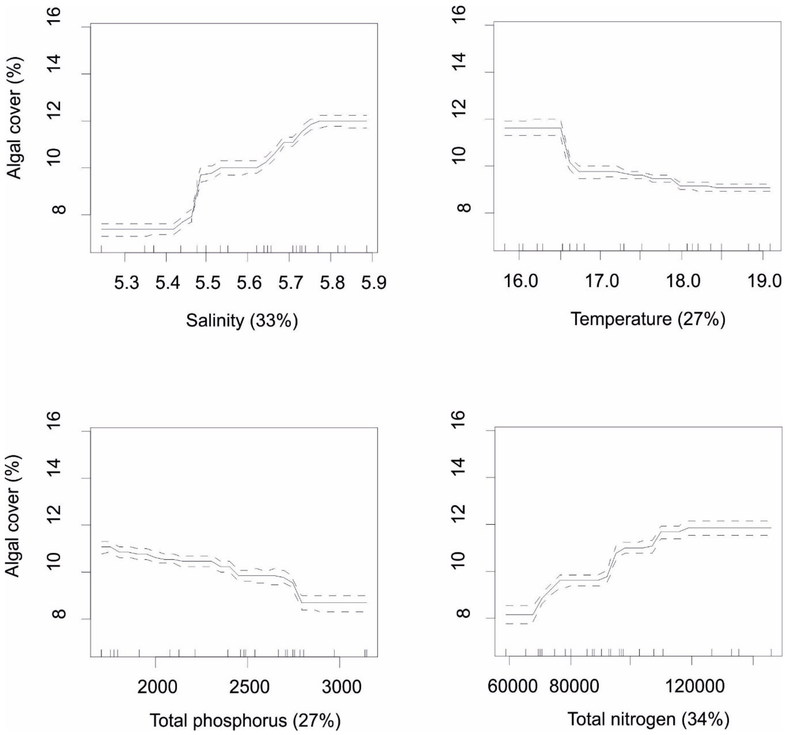
Ecological mapping using the Landsat archive showed a large within- and between-year variability of the cover of macroalgae in both study areas. Despite the large variability, a clear decline in the cover of macroalgae was observed in the late 1980s. BRT modelling showed that all studied environmental variables largely contributed to the observed variability in macroalgal cover (the variances explained in the models of Haapsalu and Small Strait were 0.663 and 0.678, respectively). Both areas were characterized by similar responses to the environmental variables, in terms of the direction of effects (
Figure 7 and
Figure 8).
Figure 7 and
Figure 8 show that increasing salinity and nitrogen loading were associated with higher cover of macroalgae, whereas the opposite was true for water temperature and phosphorus loading. As a difference among areas, the effect of temperature was much stronger in Haapsalu Bay, compared to Small Strait.
4. Discussion
In the Baltic Sea region, spatial patterns and temporal trends of macrophyte coverage are determined by natural processes (e.g., temperature and salinity trends, physical disturbances due to ice cover, and storms) and human activities (e.g., mostly land-based nutrient loading) [
36,
37]. Although heavy winter storms and sea ice regularly clean the seabed over extensive areas, the vegetation mostly recovers during spring and summer. Therefore, the resulting large-scale patterns in total macrophyte cover are broadly defined by the yearly nutrient loading and summertime hydrological conditions in the study area.
Large-scale dynamics of the patterns of macrophytes are mostly not known, because traditional field observations are very small scale, and cover only limited seascape areas and narrow time frames. Here, we linked the time series of macrophyte coverage obtained using the classification scheme of the current study to the key environmental variables known to drive the spatial and temporal patterns of macrophytes in the region, in order to demonstrate the ecological relevance of the Landsat time series. The BRT analyses showed a very good fit between remotely obtained data on macroalgal cover, hydrological, and nutrient loading. Salinity of both areas is low and macroalgal species are composed of a mixture of marine, brackish, and freshwater species. It is therefore expected that significant alteration in salinity would result in changes in the proportion of macroalgal species of different origin and shifts in the total cover of macroalgae [
23]. In general, in the study area, the reduction of salinity is manifested by the loss of many macroalgal species of marine origin, and thereby the reduction of total algal cover.
Haapsalu Bay is more eutrophicated than the Small Strait. Remote sensing effectively captured this difference, as the areal estimate of macroalgal cover was higher in Haapsalu Bay than in the Small Strait. In the BRT models, elevated nitrogen load and reduced phosphorus load were associated with the increased coverage of macroalgae. A moderate increase in nutrient concentration is often accompanied by an increase in perennial algae and opportunistic filamentous algae; however, too high loading (e.g., mostly manifested by elevated phosphorus load in the study area) is expected to negatively affect perennial species [
38,
39]. Such a relationship is explained by the higher nutrient uptake of annual algae compared to perennial algae at high nutrient concentrations, as well as the impoverishment of light conditions for perennial species [
38,
40,
41].
Moreover, the remote sensing also captured a notable shift in the cover of macroalgae in both study areas in the late 1980s. Interestingly, this period matches exactly with the timing of the most important regime shift, both in terrestrial and aquatic systems, in the Estonian climate over the past 50 years [
32]. Seemingly, a large share of the observed variability in the cover of macroalgae is determined by regional processes rather than local processes [
42], as temporal trends in the cover macrophytes were very similar in both studied areas (
Figure 6).
Due to the lack of historical records, [
32] did not involve any benthic ecology time series (including macroalgae) from the marine environment. Although the sensitivity and resolution of the Landsat archive is believed to be limited for water remote sensing, results of the current study demonstrate high utility of such long-term missions to show the patterns and dynamics of benthic vegetation over the 30 years. This approach enables us to retrospectively quantify the long-term dynamics of macroalgae in unstudied areas, and to assess the magnitude and direction of impacts of human activities and climate change in different coastal ecosystems. This is important, as we are observing widespread habitat loss and degradation in coastal marine systems worldwide, and we still lack efficient conservation measures at large scales to protect these valuable ecosystems from multiple human activities and climate change [
6].
In the Baltic Sea region, Estonia has one of the most systematically and longest collected monitoring line of macroalgal habitats. Nevertheless, these time series go back only to the mid-1990s, and involve five study sites sampled once a year during summer. Thus, remote sensing or similar methods must be used to map large areas, as, even in well-monitored regions, it is not realistic to collect more in situ spatial data. Importantly, remote sensing enables us to characterize the large-scale dynamics of macroalgal coverage which cannot be obtained from traditional sampling campaigns that collect data at limited points within a larger spatial and temporal scale. Ultimately, we can get better understanding on environmental drivers affecting macroalgal habitats at seascape scale. Nevertheless, in situ data remains a very valuable source to validate remote sensing data and to collect species information that is not visible with remote sensing. The launch of Sentinel-2 with a spatial resolution of 10 meters, and including several extra bands at 20 m resolution, opened new opportunities for the mapping of benthic algal cover [
43]. With Sentinel-2A and 2B units in orbit, the revisit time would be 2–3 days at the latitude of Estonia. This significantly increases the chance of getting cloud-free imagery, as well as provides an opportunity to start studying seasonality in macroalgal cover.


