Abstract
The Clouds and the Earth’s Radiant Energy System (CERES) Energy Balanced and Filled (EBAF) Edition 4.1 data product provides global surface irradiances. Uncertainties in the global and regional monthly and annual mean all-sky net shortwave, longwave, and shortwave plus longwave (total) irradiances are estimated using ground-based observations. Error covariance is derived from surface irradiance sensitivity to surface, atmospheric, cloud and aerosol property perturbations. Uncertainties in global annual mean net shortwave, longwave, and total irradiances at the surface are, respectively, 5.7 Wm−2, 6.7 Wm−2, and 9.7 Wm−2. In addition, the uncertainty in surface downward irradiance monthly anomalies and their trends are estimated based on the difference derived from EBAF surface irradiances and observations. The uncertainty in the decadal trend suggests that when differences of decadal global mean downward shortwave and longwave irradiances are, respectively, greater than 0.45 Wm−2 and 0.52 Wm−2, the difference is larger than 1σ uncertainties. However, surface irradiance observation sites are located predominately over tropical oceans and the northern hemisphere mid-latitude. As a consequence, the effect of a discontinuity introduced by using multiple geostationary satellites in deriving cloud properties is likely to be excluded from these trend and decadal change uncertainty estimates. Nevertheless, the monthly anomaly timeseries of radiative cooling in the atmosphere (multiplied by −1) agrees reasonably well with the anomaly time series of diabatic heating derived from global mean precipitation and sensible heat flux with a correlation coefficient of 0.46.
1. Introduction
Earth radiation budget observations by Clouds and the Earth’s Radiant Energy System (CERES) instruments started in March 2000. With more than 20 years of data currently available, the dataset will likely be used for investigations of radiation budget changes with time. Earlier studies show that the inter-annual variability of net top-of-atmosphere irradiances agree with the variability of the ocean heating rate derived from in situ ocean temperature measurements [1]. In addition, top-of-atmosphere shortwave irradiances derived from CERES instruments show large negative global monthly anomalies after 2014 [2]. Because top-of atmosphere irradiances are derived from radiance observations directly using scene-dependent angular distribution models [3], uncertainty (bias with unknown sign) in top-of-atmosphere TOA monthly mean irradiances is primarily driven by the calibration of CERES instruments [4].
Unlike TOA irradiances, surface irradiances are weakly constrained by broadband radiation observations. For example, although cloud and aerosol properties are derived from Moderate Resolution Imaging Spectroradiometer (MODIS) and geostationary satellites in producing surface irradiances included in CERES data products (e.g., SYN1deg, [5]), computed irradiances do not use CERES observations as inputs. CERES-derived TOA irradiances are used in the final process to adjust atmosphere, cloud and aerosol properties that are used for the initial computations of surface irradiances [6]. Even when computed surface irradiances are constrained by CERES-derived TOA irradiances in the final process, the correlation between surface longwave irradiances and TOA irradiances is weaker than the correlation between surface shortwave irradiances and TOA irradiances because surface longwave irradiances are largely driven by near surface temperature and specific humidity. As a consequence, computed surface irradiances are more vulnerable to artifacts caused by instruments (e.g., viewing zenith angle-dependent sensitivity, saturation, no sensitivity under opaque clouds, etc.), retrieval algorithms (e.g., assumptions in algorithms), and the input data products (e.g., inconsistency of meteorological variables used in data products) used for the computations. In addition, as the length of surface radiation budget record increases, the time series is constructed with observations taken by different sets of instruments. For example, cloud diurnal cycles used for surface irradiance computations are derived from geostationary satellites. Instrument specification differences among geostationary satellites, especially the arrival of a new generation of geostationary satellites, such as Himawari-8, GOES-16, and GOES-17, are likely to introduce spatial and temporal discontinuities when cloud properties derived from their observations are combined with those derived from existing geostationary satellites.
In this paper, we estimate the uncertainty in regional mean surface irradiances and trends derived from Edition 4.1 Energy Balanced and Filled (EBAF) surface irradiances using surface observations. We also show how the new generation of geostationary satellites affects the time series of surface irradiances. Even though the uncertainty can be quantified, we demonstrate the difficulty in quantifying the effect of combining multiple instruments on the surface irradiance anomaly time series, show the limitations of surface observations used as validation of satellite data products, and describe the various issues encountered when building a long-term surface radiation budget climate data record with multiple satellite observations. Section 2 discusses the uncertainty in regional mean net surface irradiances estimated including error correlations and uncertainty in surface anomaly time series. Section 3 shows the effect of introducing Himawari-8 observations to existing geostationary satellites. Section 4 discusses issues in the production of a surface radiation budget climate data record.
2. Uncertainty Estimate
In this section, we estimate uncertainty in computed surface irradiances and their trends. The uncertainty in downward and upward surface irradiances is estimated in Kato et al. [6]. We extend the study to net surface irradiances by taking into account error covariance between upward and downward irradiances, as well as between shortwave and longwave irradiances in Section 2.1. We use the Edition 4.1 CERES EBAF data product for the estimate. The description of the data product is given by Kato et al. [6]. We also estimate the uncertainty in surface irradiance anomalies and their trends in Section 2.2. Throughout this analysis we use the difference of observed and computed irradiance anomalies and their trends as uncertainties.
Buoys and land surface sites where surface irradiance measurements were taken are shown in Figure 1. The sites include 17 sites from the Baseline Surface Radiation Network (BSRN, [7,8]), 8 surface sites come from NOAA’s Global Monitoring Division (GMD) and SURFRAD network [9], 5 surface sites come from the US Dept. of Energy’s Atmospheric Radiation Measurement (ARM) program [10]. Buoy observations come from separate projects including the Upper Ocean Processes group at Woods Hole Oceanographic Institute maintain the Stratus, North Tropical Atlantic Site (NTAS) and Hawaii Ocean Time Series (HOTS) buoys. In addition, buoys include the Tropical Atmosphere Ocean/Triangle Trans-Ocean Buoy Network (TAO/TRITON), the Prediction and Research Moored Array in the Tropical Atlantic (PIRATA), the Research Moored Array for African-Asian-Australian Monsoon Analysis and Prediction (RAMA) in the Indian Ocean, and the Kuroshio Current and PAPA buoy sites.
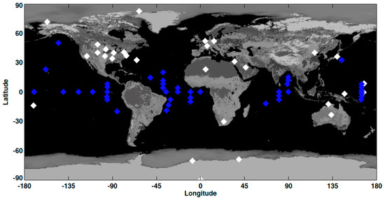
Figure 1.
Geolocations of 43 buoys (blue diamond) and 30 land-surface sites (white diamond) where downward irradiances used in validation were taken (after Rutan et al. [5]).
2.1. Uncertainty in the Net Surface and Atmospheric Irradiances
Monthly mean surface downward irradiances from the EBAF-surface product agree with observations to within 5 Wm−2 for shortwave and 2 Wm−2 for longwave when monthly mean irradiances are averaged over 46 ocean and 36 land sites [6] (uncertainties shown under global annual in Table 1). These are within the reported uncertainty of observed surface irradiances of ~5 Wm−2 [11,12,13,14,15,16]. However, the world infrared standard group calibration that is used to calibrate BSRN pyrgeometers is biased low up to 5 Wm−2 depending on column water vapor amount (i.e., revising the calibration increases longwave irradiances up to 5 Wm−2) [16]. Although the correction of archived longwave irradiance is not straightforward, the work is in progress [16].

Table 1.
Uncertainty in regional (1° × 1°) monthly and global annual downward, upward, and net shortwave, longwave, and total surface irradiances.
Previously, uncertainty in the net surface irradiance has been estimated with the assumption that errors in four irradiance components used to compute the net irradiance are perfectly correlated or uncorrelated [17]. Although the correlation is not perfect, we expect that errors are correlated because variables (e.g., temperature, specific humidity, clouds, and aerosols) that affect downward irradiances also affect upward irradiances. To estimate the covariance of surface irradiance errors, we need the sensitivity of surface irradiance components to atmospheric, cloud and surface properties. To understand the sensitivity, we utilize the adjustment of surface irradiance components used in the final process of producing the EBAF-surface irradiances. As mentioned earlier, atmospheric, surface, cloud, and aerosol properties are adjusted to match CERES-derived TOA shortwave and longwave irradiances. Subsequently, adjustments of surface irradiances are computed with the adjustments of atmospheric, cloud, aerosols, and surface properties multiplied by their respective radiative kernels [18]. If we consider that the adjustments of atmospheric, surface, cloud, and aerosol properties are to correct their bias, adjustments to the surface irradiances contains the information of how errors in atmospheric, surface cloud, and aerosol properties affect all surface irradiance components.
Table 1 shows correlation coefficients of regional and global monthly mean perturbations of surface irradiances along with uncertainties of surface irradiances from Kato et al. [6]. Because the correlation coefficient depends on region (Appendix A), temporal regional correlation coefficients are computed with upward and downward or shortwave and longwave monthly mean irradiance adjustments for every 1° × 1°grid box using 16 years of data from March 2000 through February 2016. Resulting correlation coefficients for 1° × 1° grids are averaged over different regions, separated into ocean and land. Ocean is defined as the percentage of ocean area greater than or equal to 90% in an equal area grid box [19]. Land is defined as percentages with permanent snow and oceans are, respectively, less than or equal to 10% and less than 90%. Latitudes greater than 75° are excluded in computing values in Table 1 because of the large variability of surface albedo with season. Similarly, correlation coefficients for global mean adjustments are computed by averaging adjustments of surface irradiance components globally and then computing temporal correlation coefficients with averaged adjustments using the 16 years of data.
The uncertainty U in the net irradiance is (e.g., [20] (Section 4))
where F indicates the surface irradiance, r is the correlation coefficient between upward and downward irradiance adjustments, subscript x is either shortwave or longwave, and superscripts and indicate, respectively, upward and downward irradiances. Similarly, the uncertainty in net shortwave plus longwave (total) irradiance is
where rnet is the correlation coefficient between net shortwave and net longwave irradiance adjustments. Resulting uncertainties are listed in Table 1. The regional uncertainty of monthly surface net shortwave and longwave irradiances are, respectively, 5 Wm−2 and 13 Wm−2 over ocean and 20 Wm−2 and 21 Wm−2 over land. These uncertainties combined with correlation coefficients between shortwave and longwave net irradiance adjustments lead to the uncertainty of monthly mean regional net total surface irradiance of 13 Wm−2 over ocean and 30 Wm−2 over land. When global annual mean irradiances combined with correlation coefficients are used in a similar way, the uncertainty in the annual global net total irradiance is 10 Wm−2 (Table 1).
In order to estimate the uncertainty in regional net atmospheric irradiance defined as the net TOA irradiance minus net surface irradiance, we need the uncertainty in regional TOA irradiances. The uncertainty in regional TOA irradiances estimated by Loeb et al. [2] is caused by three sources, (1) diurnal correction, (2) radiance to irradiance conversion, and (3) CERES instrument calibration. The uncertainty in regional TOA shortwave irradiance due to diurnal correction is 1.9 Wm−2. The irradiance conversion error is 1 Wm−2 [3] and instrument calibration uncertainty is 1% (1σ) or 1 Wm−2. When these uncertainties are used, the uncertainty in regional TOA shortwave irradiance is approximately 2.5 Wm−2 [2]. Similar to the shortwave, the uncertainty in regional TOA longwave irradiance is also 2.5 Wm−2. If shortwave and longwave errors are independent and the uncertainty in insolation is ignored, the uncertainty in the regional net TOA irradiance is 3.5 Wm−2.
If errors in net TOA and surface irradiances are independent, the uncertainty in the regional net atmospheric irradiance over ocean is (13.02 + 3.52)1/2 = 13.5 Wm−2. While this gives mean uncertainty in regional monthly net atmospheric irradiance, uncertainty in the surface and TOA irradiance highly depends on region. Because most buoys and land sites used for validation of EBAF-surface irradiances are, respectively, in the tropics and mid-latitudes (Figure 1), the uncertainty over ocean likely represents tropical ocean and the uncertainty over land likely represents midlatitude land.
2.2. Uncertainty in Surface Irradiance Trend and in Observing Decadal Surface Irradiance Change
Similar to the uncertainty estimate in monthly mean net surface irradiances, we use surface observations to estimate the uncertainty in anomalies and trends derived from EBAF monthly mean surface irradiances. With use of the uncertainty in the trends, we also determine the uncertainty in inferring decadal surface irradiance change. The first step is to compare anomaly time series calculated with computed and observed surface irradiances. One issue in deriving anomaly time series from observed surface irradiances is that surface observations taken at most sites cover only a part of the 20-year time period of CERES observations. Therefore, constructing anomaly time series with surface observations for the entire time period of CERES observations and comparing with the time series derived from EBAF surface irradiances requires multiple steps. If a time series of observed surface irradiances is derived by combining all surface sites, the variability might be driven by the number of sites changing with time. Because the climatological mean surface irradiance depends on geolocation, it should be subtracted from the corresponding monthly mean irradiance at each site to compute the anomaly. Therefore, we first deseasonalize the observed downward shortwave or longwave irradiances , where x indicates either shortwave or longwave, at each site by subtracting climatological monthly mean irradiances ,
where and subscripts i and j indicate, respectively, each month and site. Second, we divide the anomaly time series at each site by its standard deviation of anomalies. Third, for a given month, we add all available normalized anomalies and divide by the square root of the number of available sites. Fourth, we divide resulting mean anomalies by their standard deviation and multiply by the standard deviation of monthly anomalies over global land, ocean or land+ocean computed with the EBAF-surface product σg. The second through fourth steps are, therefore,
where m is the number of available sites for the month ti, and . The anomaly time series from the EBAF-surface product is also derived in the same way by matching geolocations and time periods of surface observations.
Because geolocation-dependent mean surface irradiance at available sites is removed in the first deseasonalizing process, this method is less prone to be affected by a variable number of sites. However, if the observation time series at one site is composed of multiple instruments (as is the case at buoy locations), calibration differences among the instruments can introduce artifacts. Even when one instrument is used, frequent calibration is necessary to avoid calibration drift [16]. It is difficult to unambiguously determine whether an unusually large anomaly is real or due to an instrument problem. Therefore, we do not apply any screening by the size of anomalies. Instead, we require for surface observations to be included in the time series: (1) at a given site and a month, instruments need to be operated more than 90% of the month and (2) multiple years (more than two years) of observations need to be available for a given site to assure reasonable ability to deseasonalize the monthly mean values.
While this method produces time series by minimizing the impact of variable number of sites, the trend derived from the combined time series by linear regression is not the same as the mean slopes derived from individual sites. If all sites have the same observation length, cover the entire time series, and all sites have the same trend, then the trend derived from combined time series is the square root of the number of sites times the trend. Other than this ideal case, the trend of combined monthly anomalies depends on record lengths and time of observation periods of individual sites, in addition to trends at individual sites. For land time series, 17 and 18 out of 30 sites cover at least 80% of the 19-year shortwave and longwave time period (228 months), respectively. Therefore, the trend of the combined time series is primarily driven by trends that exist in observations (real or not), not by variable number of sites with time. Observation lengths over oceans are shorter. However, as shown later in this Section, differences in the time series derived from observations and EBAF over oceans are similar to those derived over land, suggesting that the trend of combined time series over oceans is also driven by trends in observations.
Figure 2 and Figure 3 show, respectively, downward shortwave and downward longwave monthly irradiance anomaly time series derived with this method for ocean plus land (a), ocean (b), and land (c). Generally, EBAF time series correlate quite well with observed time series, particularly the land time series with a correlation coefficient near 0.88. Distributions of correlation coefficients derived from individual sites are discussed in Appendix B. The root-mean-square (RMS) difference of observed and EBAF anomalies are shown in Table 2. The RMS difference may be considered as the uncertainty in EBAF downward irradiance anomalies. The trends of downward longwave irradiance over ocean (Figure 3b) and shortwave irradiance over land (Figure 2c) derived from EBAF anomaly time series are within the 95% confidence interval of the trend derived from observed anomaly time series. Using EBAF and observed time series, we estimate the uncertainty in the trend derived from EBAF anomaly time series by sum of the difference of slopes derived from EBAF and observations and uncertainty of the slope derived from EBAF and observations,
where b is the slope of the linear regression line, and are defined as [21]
Fi,x,anom is the monthly anomaly of irradiance x, t is the number of months counted from the beginning of the time series, and a is the intercept of the linear regression line and subscript y is either EBAF or obs. Slopes derived from EBAF and observed surface deseasonalized anomalies as well as 95% confidence interval (2σ) of the slopes are shown in Table 2. In Equation (5), in addition to the difference of slopes estimated from EBAF and observations (first term on the right side of Equation (5)), the measure of goodness of fit to EBAF (second term on the right side of Equation (5)) and observed (third term on the right side of Equation (5)) anomalies defined by Equation (6) are added based on the confidence interval. Equation (6) states that if the record length n is sufficiently long (e.g., 20 years or longer), then the uncertainty of the slope of the linear regression is proportional to the standard deviation of irradiance deseasonalized anomalies and inversely proportional to Therefore, the second and third terms on the right side of Equation (5) become small compared to the first term as the time series gets longer.
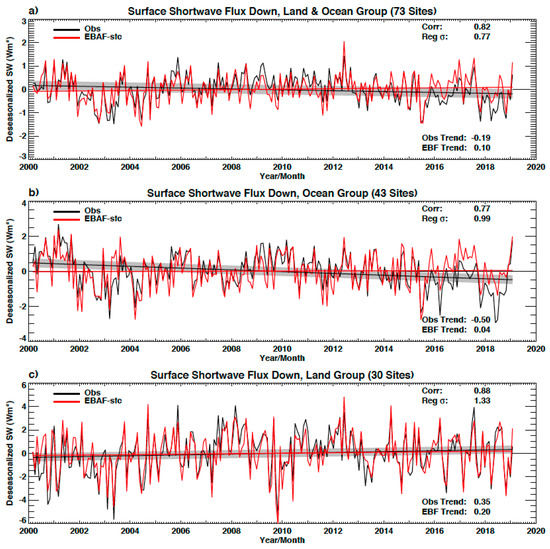
Figure 2.
(a) Deseasonalized monthly surface downward shortwave anomalies computed with observed irradiances shown at 43 buoys and 30 land sites. Black and red lines are observed and energy balanced and filled (EBAF)-computed irradiance anomalies. Linear regression lines are also shown with the same color. A 95% confidence interval of the observed trend is shown by shade. “Corr” and “Reg(ional)” indicate correlation coefficient and standard deviation. The slope of the linear regression line shown on bottom right is Wm−2 decade−1. (b,c) plots show anomaly time series for, respectively, 43 buoys and 30 land sites separately.
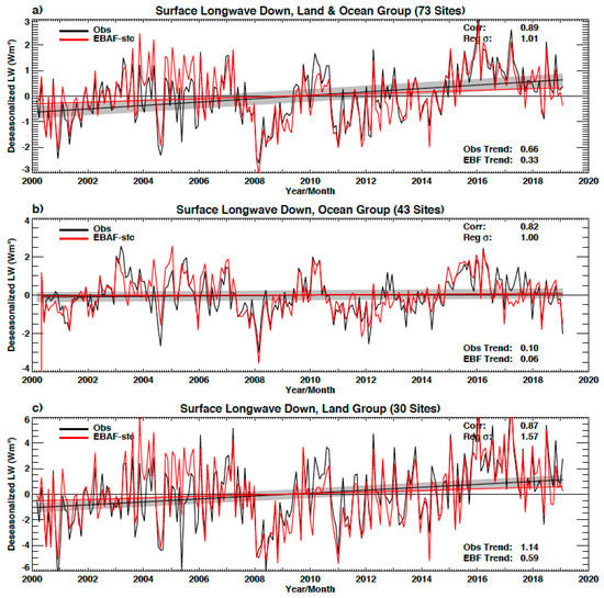
Figure 3.
(a–c) Same as Figure 1 but for downward longwave irradiance.

Table 2.
Surface downward shortwave and longwave anomaly root-mean-square (RMS) differences, trends and their 95% confidence intervals.
Table 3 shows the uncertainty computed with Equation (5). The downward longwave irradiance over ocean, shortwave irradiance over land, and downward shortwave irradiance over land+ocean values are less than 0.5 Wm−2 per decade. If we assume that the uncertainties in anomalies for both decades are the same and the error in the first decade is not correlated with the error in the second decade, the uncertainty (1σ) in detecting the change with two decadal mean irradiances is times the uncertainty of the slope, i.e., . Therefore, if differences of decadal global mean downward shortwave and longwave irradiances are, respectively, greater than 0.45 Wm−2 and 0.52 Wm−2, then the difference is significant.

Table 3.
Trend error and overall uncertainty in estimating trend in Wm−2 decade−1.
For the time series of 20 years, the uncertainty caused by linear regression (the second and third terms on the right side of Equation (5)) is small so that given by Equation (5) is dominated by the slope difference between EBAF and observed anomalies. The measure of goodness of fit represents how well the liner regression line represents the trend, assuming that anomalies are correct. However, if the goal is to evaluate anomalies and their trend, the goodness of fit is not a measure of the uncertainty. We need separate data to assess the uncertainty in anomalies. We used surface observations to assess the uncertainty in EBAF surface irradiance anomalies [6]. Comparisons with surface observations are one way to assess the error in satellite derived surface irradiances and their trends. In the next section, however, we show that there is a limitation of surface observations in evaluating computed surface irradiances.
3. Impact of New Generation Geostationary Satellites on Compute Surface Irradiances
Although we used surface observations to estimate the uncertainty in Section 2.1 and Section 2.2, the number of surface observation sites is limited. In addition, land sites are located predominately in the northern hemisphere mid-latitudes and the buoys are located in the tropics. In this section, we demonstrate the consequence of using the limited number of surface sites in estimating the uncertainty in trends.
New generation geostationary satellites with a MODIS-like imager (i.e., an imager with many spectral channels) are replacing existing geostationary satellites with fewer channels. Those new generation geostationary satellites include Himawari-8, GOES-16, and GOES-17. Himawari-8 replaced MTSAT-2 on July 6 2015. GOES-16 replaced GOES-14 on January 1 2018. These satellites are used in producing surface irradiance for CERES data products by providing the diurnal cycle of cloud fraction, optical thickness, emissivity, top temperature, top and base heights, phase, and particle size [22,23,24,25]. Differences depend on cloud type, but generally cloud fraction derived from Himawari-8 is larger than the cloud fraction derived from MTSAT-2. In addition, visible cloud optical thickness, IR emissivity and cloud top temperature derived from Himawari-8 are smaller than those derived from MTSAT-2. Optically thinner clouds, in part, compensate for larger cloud fraction, resulting in a smaller downward shortwave irradiance discontinuity. However, the combined effect of higher cloud top heights (i.e., smaller cloud top pressures) and optically thinner clouds is higher cloud top bases. As a result, downward longwave irradiances computed with cloud properties derived from Himawari-8 are smaller than downward irradiances computed with cloud properties derived from MTSAT-2, especially over regions with large viewing zenith angles (i.e., from mid-latitude to 60° latitude, Figure 4). Although the effect is apparent in the regional map shown in Figure 4, the exact error in regional downward surface irradiances is difficult to quantify. This is because, as Figure 4 shows, some of differences are real. For example, anomalies shown around 60° S over the Pacific are not entirely caused by the MTSAT-2 to Himawari-8 difference. Although the broader feature following the geostationary boundary is an artifact, smaller spatial scale anomalies are due to clouds. Quantification of the error in monthly anomalies of the downward longwave irradiance is, therefore, difficult. Similar to the mean surface irradiances, some of the large changes in the downward longwave irradiance in a time series appears to be real. For example, a large decrease in the global monthly downward longwave irradiance anomalies that occurred after March 2016 in the anomaly time series shown in Figure 5 is largely due to the end of a strong El Nino.
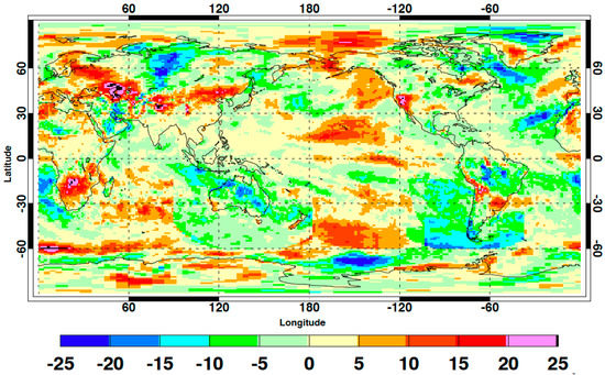
Figure 4.
Regional anomalies of longwave surface downward irradiance in Wm−2 for July 2018. Anomalies are computed as the difference between July 2018 regional downward longwave irradiance minus regional July downward longwave irradiance climatology (average from July 2005 through June 2015). Himawar-8 covers 60°N–60°S 90°E–180°E and GOES-16 covers 60°N–60°S 35°W–105°W.
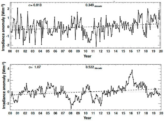
Figure 5.
Global monthly deseasonalized anomaly time series of surface downward (top) shortwave and (bottom) longwave irradiances. Two numbers shown at the top of each plot are the standard deviation of anomalies (σ) and slope regression line (dashed line).
To understand a potential impact of Himawari-8 on the regional monthly anomaly time series, Figure 6 shows the comparison of downward longwave and shortwave irradiance monthly anomalies using EBAF irradiances and observed irradiances at buoys located within the region where Himawari-8 observations are used to derive cloud properties. The result indicates that the effect of MTSAT2 to Himawari-8 in July 2015 is not decisively apparent, probably because the variability is large compared with the downward longwave anomaly discontinuity. In addition, the systematic differences occur predominately in southern hemisphere mid-latitude to 60°S over ocean where surface sites are absent. However, as multiple new generation geostationary satellites are used after January 2018, the effect to the global mean downward longwave irradiance is probably inevitable. There are some approaches that can mitigate the discontinuities associated with instrument changes. Potentially, an improved time series could be realized by reducing the number of channels used in retrieving cloud properties with new generation geostationary satellites to better match older geostationary satellites. Adaption of such an approach is a trade-off between more stable time series and accurate monthly mean surface irradiances.
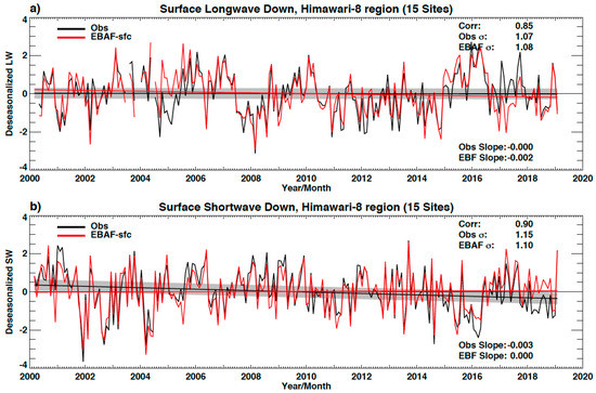
Figure 6.
Deseasonalized anomaly time series of surface downward (a) longwave and (b) shortwave irradiances from buoys and a land site within the region covered by Himawari-8. Included surface sites are, in the Pacific Ocean 8-TAO buoys, in the Indian Ocean 5-RAMA buoys, in the N Pacific the Kuroshio Current Buoy (KEO) and a ground site at Alice Springs, AU. Anomalies at individual sites are normalized by the standard deviation (see text for the detail). Black and red lines are observed and EBAF irradiance anomalies. Linear regression lines are also shown with the same color. A 95% confidence interval of the observed trend is shown by shade. Himawari-8 replaced MTSAT2 on 6 July 2015.
4. Consistency Check Using Energy Balance
While excluding all artifacts from surface radiation budget data products is very difficult in the foreseeable future, the anomaly time series of radiation budget is useful to understand how energy fluxes change with time and to assess the quality of multiple flux data products. For example, when a radiation budget time series derived from the EBAF data product is compared with an anomaly time series of diabatic heating by precipitation, the comparison can provide a quality assessment of both data products. We show one example of energy flux anomaly comparison that helps us to monitor large artifacts in producing EBAF surface irradiances.
Figure 7 shows the time series of global (90°N to 90°S) monthly anomalies of diabatic heating due to precipitation and sensible heat flux by the blue line. In addition, the red line is global monthly anomalies of net atmospheric irradiance multiplied by −1. Diabatic heating anomalies are derived from Edition 2.3 Global Precipitation Climatology Project (GPCP, [26]), surface sensible heat flux anomalies are derived from ERA5 [27], and net atmospheric irradiance anomalies are derived from Edition 4.1 EBAF data products. Standard deviations of deseasonalized anomalies with a 12-month moving window of diabatic heating due to precipitation, sensible heat flux, and net atmospheric irradiance are, respectively, 0.58 Wm−2, 0.16 Wm−2, and 0.51 Wm−2. The net annual energy input to the atmosphere is very close to 0 when fluxes are averaged over the entire globe. The balance is achieved by diabatic heating by precipitation, sensible heat flux at the surface, and radiative cooling. However, when satellite derived data products are used, the residual of the atmospheric energy balance averaged over 10 years (from July 2005 through June 2015) is −14 Wm−2, where the means of net atmospheric irradiance, diabatic heating by precipitation, and sensible heat flux are, respectively, −109 Wm−2, 78 Wm−2, and 17 Wm−2. Even though the global annual mean atmospheric energy budget derived from these products has the residual, the anomaly time series derived from GPCP+ERA5 and EBAF data products are reasonably consistent with a correlation coefficient of 0.46. Given that precipitation and radiation are derived independently from different instruments, this agreement is encouraging. As longer time series become available and more energy flux components are observed by many different instruments, the energy balance can be a useful tool to assess the quality of data products or derive missing flux components.
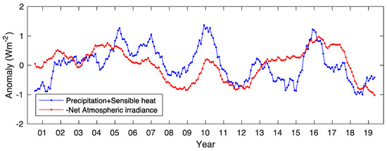
Figure 7.
Global monthly deseasonalized anomaly time series of (blue) the sum of diabatic heating due to precipitation and sensible heat flux and (red) −1 time radiative cooling in the atmosphere. Anomalies are averaged with a 12-month moving window.
5. Discussion and Conclusions
We estimated the uncertainty in regional net surface shortwave and longwave irradiances, as well as the uncertainty in the net total irradiance. We also estimated the uncertainty in anomalies, trends and in detecting changes in downward shortwave and longwave irradiances averaged over a decade. The results indicate that the uncertainty in estimating changes is much smaller than the uncertainty in mean irradiances. While the smaller uncertainty in the trends is encouraging for using surface radiation budget data products for climate studies, we do face some challenges. As the record becomes longer, it is composed of observations taken by multiple instruments. As a result, observations taken by new instruments are combined with existing observations. We showed one example of how cloud properties derived from the new generation geostationary satellites influence the downward longwave irradiance regionally. Discontinuities are apparent in a map of downward longwave irradiance anomalies. However, separating artifacts from real anomalies and quantifying artifacts is difficult. In addition, the effect on anomaly time series is even harder to quantify because of the larger variability of surface irradiance when compared with the discontinuity. Furthermore, the effect is difficult to detect in the evaluation of time series by surface observations because most surface sites are located where the effect is relatively small. As Equation (5) defines, we used the difference of the slope derived from EBAF and observed anomalies and the goodness of fit by the linear regression as the uncertainty. As the time series becomes longer, the uncertainty is dominated by the difference of the slope derived from EBAF and surface observations. We therefore emphasize the importance of having validation sites in as wide a range of geolocations as possible and provide a caveat using the trend uncertainty estimated in this study to, for example, polar regions.
The uncertainty in the trend estimated from the Edition 4.1 EBAF data product is small compared to the uncertainty in monthly mean irradiances. It is also instructive to compare this trend uncertainty to that expected under climate change scenarios. According to AR4 climate models, for a 1 K surface temperature change the net atmospheric irradiance decreases 2 Wm−2, which balances by a 1.7% to 2% precipitation change [28]. Although recent CERES observations indicate that the TOA net irradiance is increasing with time, if we assume that the TOA net irradiance does not change, net surface irradiance needs to decrease 2 Wm−2 per 1 K surface temperature increase. A study by Ramaswamy et al. [29] indicates that global mean net surface irradiance change is predominately due to the net longwave irradiance change. For the surface temperature of 290 K, the upward longwave irradiance increases by 5.5 Wm−2, which suggests that the downward longwave irradiance increases by 3.5 Wm−2 per 1 K increase of surface temperature. The surface temperature increases with a rate of 0.2 K per decade under the Representative Concentration Pathway (RCP) 6.0 scenario [30], which gives a rate of increase of 0.7 Wm−2 global mean downward longwave irradiance per decade. The uncertainty in estimating decadal change of downward longwave irradiance derived in Section 2.2 is smaller than the predicted decadal change of global mean downward longwave irradiance change. We must, however, mitigate the discontinuity caused by changing instruments.
Author Contributions
Conceptualization, S.K. and D.A.R.; methodology, S.K. and D.A.R.; software, D.A.R., F.G.R., T.E.C., S.-H.H., A.R., T.J.T. and D.F.; validation, D.A.R., A.V.-M.; formal analysis, S.K., D.A.R. and F.G.R.; writing—original draft preparation, S.K.; writing—review and editing, D.A.R., S.-H.H., T.J.T., X.H. All authors have read and agreed to the published version of the manuscript.
Funding
This research has been supported by the NASA Clouds and he Earth’s Radiant Energy System project.
Acknowledgments
We would like to thank the Editor Norman Loeb and William Smith Jr. for helpful discussions. The Ed4.1 CERES EBAF-surface (doi:10.5067/TERRA+AQUA/CERES/EBAF-SURFACE_L3B004.0) EBAF–TOA (doi:10.5067/TERRA+AQUA/CERES/EBAF-TOA_L3B004.0), and SYN1deg-Month (doi:10.5067/TERRA+AQUA/CERES/SYN1degMonth_L3.004) dataset was downloaded from https://ceres.larc.nasa.gov/order_data.php. Surface observations of downward irradiances were collected from a number of sources. For land-based observations we include 17 sites from the Baseline Surface Radiation Network (BSRN, [7,8]), available at www.bsrn.de. Eight surface sites come from NOAA’s Global Monitoring Division (GMD) and SURFRAD network at NOAA’s Air Resources Laboratory/Surface Radiation Research Branch [9], and are available from www.esrl.noaa.gov/gmd/grad. Five surface sites come from the US Dept. of Energy’s Atmospheric Radiation Measurement (ARM) program and are available from www.arm.gov/data. Buoy observations come from two sources though separate projects. The Upper Ocean Processes group at Woods Hole Oceanographic Institute maintain the Stratus, North Tropical Atlantic Site (NTAS) and Hawaii Ocean Time Series (HOTS) buoys providing valuable time series of observations in climatically important regions of the ocean. Data are available at http://uop.whoi.edu/. We would also like to acknowledge the Tropical Atmosphere Ocean/Triangle Trans-Ocean Buoy Network (TAO/TRITON) Project Office of NOAA’s Pacific Marine Environmental Labs (PMEL) where three groups of buoy data were downloaded: In the Pacific, the TAO/TRITON data, from the tropical Atlantic Ocean, the Prediction and Research Moored Array in the Tropical Atlantic (PIRATA), the Research Moored Array for African-Asian-Australian Monsoon Analysis and Prediction (RAMA) in the Indian Ocean, and the Kuroshio Current and PAPA buoy sites. All data are made available at www.pmel.noaa.gov/.
Conflicts of Interest
The authors declare no conflict of interest.
Appendix A
As discussed in Section 2.1, perturbations of upward and downward surface irradiances corresponding atmospheric, surface, cloud, and aerosol properties are computed by radiative kernels. Perturbations are computed regionally in 1° × 1° grids over 16 years from March 2000 through February 2016. Figure A1 shows temporal correlation coefficients of shortwave downward and upward irradiance perturbations, longwave downward and upward irradiance perturbations, and shortwave and longwave net perturbations. If the uncertainty in surface properties (albedo or emissivity) is small, such as shortwave over ocean, the correlations of downward and upward irradiance perturbations are large because uncertainty in atmosphere, cloud, and aerosol properties affect both downward and upward irradiances. When the uncertainty in surface properties is large, however, the correlation coefficient is small. Therefore, correlation coefficients over land for both shortwave and longwave tend to be smaller than those over ocean.
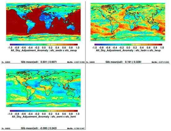
Figure A1.
Temporal correlation coefficients of (top left) shortwave downward and upward irradiance perturbations, (top right) longwave downward and upward irradiance perturbations, and (bottom left) shortwave and longwave net perturbations in 1° × 1° grids. Sixteen years of data from March 2000 through February 2016 are used.
Appendix B
Combined anomaly time series are used in Section 2.2. In this appendix, we show the difference of correlation coefficients, anomalies, and their slopes derived from observations and EBAF at individual sites (Figure A2 and Figure A3). Anomaly time series derived for individual sites are not normalized by the standard deviation of anomalies.
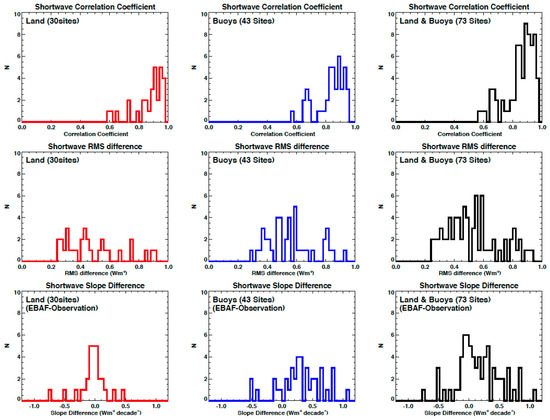
Figure A2.
Histogram of (top row) correlation coefficients, (middle row) root-mean-square (RMS) differences, and (bottom row) slope differences derived from ground-based observations and EBAF at individual sites for downward shortwave irradiance anomalies.
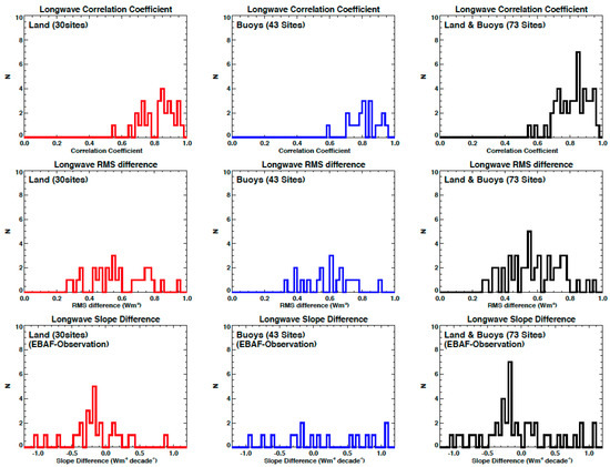
Figure A3.
Same as Figure A2 but for downward longwave irradiance anomalies.
References
- Johnson, G.C.; Lyman, J.M.; Loeb, N.G. Loeb, Improving estimates of Earth’s energy imbalance. Nat. Clim. Chang. 2016, 6, 639–640. [Google Scholar] [CrossRef]
- Loeb, N.G.; Doelling, D.R.; Wang, H.; Su, W.; Nguyen, C.; Corbett, J.G.; Liang, L.; Mitrescu, C.; Rose, F.G.; Kato, S. Clouds and the Earth’s Radiant Energy System (CERES) Energy Balanced and Filled (EBAF) top-of-atmosphere (TOA) Edition-4.0 data product. J. Clim. 2018, 31, 895–918. [Google Scholar] [CrossRef]
- Su, W.; Corbett, J.; Eitzen, Z.; Liang, L. Next-generation angular distribution models for top-of-atmosphere radiative flux calculation from CERES instruments: Validation. Atmos. Meas. Tech. 2015, 8. [Google Scholar] [CrossRef]
- Loeb, N.G.; Wielicki, B.A.; Doelling, D.R.; Smith, G.L.; Keyes, D.F.; Kato, S.; Manalo-Smith, N.; Wong, T. Toward optimal closure of the Earth’s top-of-atmosphere radiation budget. J. Clim. 2009, 22, 748–766. [Google Scholar] [CrossRef]
- Rutan, D.A.; Kato, S.; Doelling, D.R.; Rose, F.G.; Nguyen, L.T.; Caldwell, T.E.; Loeb, N.G. CERES synoptic product: Methodology and validation of surface radiant flux. J. Atmos. Ocean. Technol. 2015, 32, 1121–1143. [Google Scholar] [CrossRef]
- Kato, S.; Rose, F.G.; Rutan, D.A.; Thorsen, T.J.; Loeb, N.G.; Doelling, D.R.; Huang, X.; Smith, W.L.; Su, W.; Ham, S.-H. Surface irradiances of Edition 4.0 Clouds and the Earth’s Radiant Energy System (CERES) Energy Balanced and Filled (EBAF) data product. J. Clim. 2018, 31. [Google Scholar] [CrossRef]
- Ohmura, A.; Dutton, E.; Forgan, B.; Frohlich, C.; Gilgen, H.; Hegne, H.; Heimo, A.; Konig-Langlo, G.; McArthur, B.; Muller, G.; et al. Baseline Surface Radiation Network (BSRN/WCRP): New precision radiometry for climate change research. Bull. Am. Meteorol. Soc. 1998, 79, 2115–2136. [Google Scholar] [CrossRef]
- Driemel, A.; Augustine, J.; Behrens, K.; Colle, S.; Cox, C.; Cuevas-Agulló, E.; Denn, F.M.; Duprat, T.; Fukuda, M.; Grobe, H.; et al. Baseline Surface Radiation Network (BSRN): Structure and data description (1992-2017). Earth Syst. Sci. Data 2018, 1491–1501. [Google Scholar] [CrossRef]
- Augustine, J.A.; DeLuisi, J.J.; Long, C.N. SURFRAD—A national surface radiation budget network for atmospheric research. Bull. Am. Met. Soc. 2000, 81, 2341–2358. [Google Scholar] [CrossRef]
- Ackerman, T.P.; Stokes, G.M. The atmospheric radiation measurement program. Phys. Today 2003, 56, 38–44. [Google Scholar] [CrossRef]
- Colbo, K.; Weller, R.A. Accuracy of the IMET sensor package in the subtropics. J. Atmos. Ocean. Technol. 2009, 26, 1867–1890. [Google Scholar] [CrossRef]
- Michalsky, J.J.; Dutton, E.; Rubes, M.; Nelson, D.; Stoffel, T.; Wesley, M.; Splitt, M.; DeLuisi, J. Optimal measurement of surface shortwave irradiance using current instrumentation. J. Atmos. Ocean. Technol. 1999, 16, 55–69. [Google Scholar] [CrossRef]
- Michalsky, J.J.; Dolce, R.; Dutton, E.G.; Haeffelin, M.; Major, G.; Schlemmer, J.A.; Slater, D.W.; Hickey, J.R.; Jeffries, W.Q.; Los, A.; et al. Results from the first ARM diffuse horizontal shortwave irradiance comparison. J. Geophys. Res. 2003, 108, 4108. [Google Scholar] [CrossRef]
- Dutton, E.G.; Long, C.N.; Wild, M.; Ohmura, A.; Groebner, J.; Roesch, A. Chapter 5: Long-Term In-Situ Surface Flux Data Products, in GEWEX Radiative Flux Assessment, Volume 1: Assessment. World Clim. Res. 2012, 12, 135–158. [Google Scholar]
- Vuilleumier, L.; Hauser, M.; Félix, C.; Vignola, F.; Blanc, P.; Kazantzidis, A.; Calpini, B. Accuracy of ground surface broadband shortwave radiation monitoring. J. Geophys. Res. Atmos. 2014, 119, 13,838–13,860. [Google Scholar] [CrossRef]
- Nyeki, S.; Wacker, S.; Grobner, J.; Finsterle, W.; Wild, M. Revising shortwave and longwave radiation archives in view of possible revisions of the WSG and WISG reference scales: Methods and implications. Atmos. Meas. Tech. 2017, 10, 2057–3068. [Google Scholar] [CrossRef]
- Kato, S.; Loeb, N.G.; Rutan, D.A.; Rose, F.G.; Sun-Mack, S.; Miller, W.F.; Chen, Y. Uncertainty estimate of surface irradiances computed with MODIS-, CALIPSO-, and CloudSat-derived cloud and aerosol properties. Surv. Geophys. 2012, 33. [Google Scholar] [CrossRef]
- Thorsen, T.J.; Kato, S.; Loeb, N.G.; Rose, F.G. Observation-Based Decomposition of Radiative Perturbations and Radiative Kernels. J. Clim. 2018, 31, 10039–10058. [Google Scholar] [CrossRef]
- Doelling, D.R.; Loeb, N.G.; Keyes, D.F.; Nordeen, M.L.; Morstad, D.; Nguyen, C.; Wielicki, B.A.; Young, D.F.; Sun, M. Geostationary enhanced temporal interpolation for CERES flux products. J. Atmos. Ocean. Technol. 2013, 30, 1072–1090. [Google Scholar] [CrossRef]
- Mandel, J. The Statistical Analysis of Experimental Data; Dover: New York, NY, USA, 1984; pp. 58–77. [Google Scholar]
- Wilks, D.S. Statistical Methods in the Atmospheric Sciences; Academic Press: Oxford, UK, 2011; pp. 215–225. [Google Scholar]
- Minnis, P.; Nguyen, L.; Palikonda, R.; Heck, P.W.; Spangenberg, D.A.; Doelling, D.R.; Ayers, J.K.; Smith, W.L., Jr.; Khaiyer, M.M.; Trepte, Q.Z.; et al. Near-real time cloud retrievals from operational and research meteorological satellites. In Proceedings of the SPIE Remote Sens. Clouds Atmos. XIII, 7107-2, Cardiff, Wales, UK, 15–18 September 2008; p. 8, ISBN 9780819473387. [Google Scholar]
- Minnis, P.; Bedka, K.; Trepte, Q.; Yost, C.R.; Bedka, S.T.; Scarino, B.; Khlopenkov, K.; Khaiyer, M.M. A consistent long-term cloud and clear-sky radiation property dataset from the Advanced Very High Resolution Radiometer (AVHRR). In Proceedings of the Climate Algorithm Theoretical Basis Document (C-ATBD), CDRP-ATBD-0826 Rev 1 AVHRR Cloud Properties—NASA, NOAA CDR Program, Silver Spring, MD, USA, 19 September 2016; p. 159. [Google Scholar] [CrossRef]
- Minnis, P.; Sun-Mack, S.; Chen, Y.; Chang, F.-L.; Yost, C.R.; Smith, W.L., Jr.; Heck, P.W.; Arduini, R.F.; Trepte, Q.Z.; Ayers, K.; et al. CERES MODIS cloud product retrievals for Edition 4, Part 1: Algorithm changes. IEEE Trans. Geosci. Remote Sens. 2020. under review. [Google Scholar]
- Trepte, Q.Z.; Minnis, P.; Sun-Mack, S.; Yost, C.R.; Chen, Y.; Jin, Z.; Hong, G.; Chang, F.-L.; Smith, W.L., Jr.; Bedka, K.; et al. Global cloud detection for CERES Edition 4 using Terra and Aqua MODIS data. IEEE Trans. Geosci. Remote Sens. 2019, 57, 9410–9449. [Google Scholar] [CrossRef]
- Adler, R.F.; Gu, G.; Huffman, G.J. Estimating climatological bias errors for the Global Precipitation Climatology Project (GPCP). J. Appl. Meteor. Climatol. 2012, 51, 84–99. [Google Scholar] [CrossRef]
- Hersbach, H.; de Rosnay, P.; Bell, B.; Schepers, D.; Simmons, A.; Soci, C.; Abdalla, S.; Alonso-Balmaseda, M.; Balsamo, G.; Bechtold, P.; et al. Operational Global Reanalysis: Progress, Future Directions and Synergies with NWP; ERA Report Series; European Centre for Medium Range Weather Forecasts: Shinfield, UK, 2018. [Google Scholar] [CrossRef]
- Held, I.M.; Soden, B.J. Robust responses of the hydrological cycle to global warming. J. Clim. 2006, 19, 5686–5699. [Google Scholar] [CrossRef]
- Ramaswamy, V.; Collins, W.; Haywood, J.; Lean, J.; Mahowald, N.; Myhre, G.; Nail, V.; Shine, K.P.; Soden, B.; Stenchikov, G.; et al. Radiatie forcing of climate: The historical evolution of the radiative forcing concept, the forcing agents and their quantification, and applications. Meteorol. Monogr. 2019, 59, 14.1–14.101. [Google Scholar] [CrossRef]
- Taylor, K.E.; Stouffer, R.J.; Meehl, G.A. An overview of CMIP5 and the experiment design. Bull. Am. Meteorol. Soc. 2012, 485–498. [Google Scholar] [CrossRef]
© 2020 by the authors. Licensee MDPI, Basel, Switzerland. This article is an open access article distributed under the terms and conditions of the Creative Commons Attribution (CC BY) license (http://creativecommons.org/licenses/by/4.0/).