Abstract
The linear structures in synthetic aperture radar (SAR) images can provide important geometric information regarding the illuminated objects. However, the linear structures of various objects sometimes disappear in traditional SAR images, which severely affects the application in automated scene analysis and information extraction techniques. This paper proposes a parametric SAR image recovery method for linear structures of extended targets. By extracting the spatial phase distribution feature in image domain, the proposed method is used to identify the endpoints among all of the scattered points in SAR images and reconstruct the disappeared linear structures based on the scattering model. The method can be generally divided into three procedures: endpoints and point targets classification, linear structures recognition, and linear structures reconstruction. In the first step, the endpoints of linear structures and point targets are classified by setting a threshold related to the spatial phase distribution feature. Afterwards, the linear structures recognition method is used to determine which two endpoints can be formed into a linear structure. Finally, the parametric scattering models are used to reconstruct the disappeared linear structures. Experiments are conducted on both computer simulations and the data that were acquired by microwave anechoic chamber experiment, tower crane radar experiment, and unmanned vehicle radar experiment in order to validate the effectiveness and robustness of the proposed method.
1. Introduction
With its all-weather, all-day, and high-resolution capabilities, synthetic aperture radar (SAR) has been widely applied in automatic targets recognition and information extraction techniques. Unlike ordinary optical images, an important feature of distributed targets in SAR images is that the scattering features are often highly varying in different observation angles.
To illustrate this phenomenon, take the linear structure as an example. Figure 1 shows the radar imaging results of a football gate at different observation angles, where E1 and E2 are the two endpoints of the crossbar, respectively. Aperture CD is directly in front of the football gate and aperture AB is on the left side of the football gate. The crossbar of the football gate can only be completely imaged when the radar sweeps over the normal direction of the crossbar shown in Figure 1d. Otherwise, the linear structure of the crossbar completely disappears, except for its endpoints in the SAR image, as shown in Figure 1c. According to the local field principle in geometric diffraction theory, under high-frequency conditions, such as radar systems, the diffraction field only depends on the physical and geometrical properties in a small area near the diffraction point [1,2]. Therefore, in SAR images, the linear structures of various targets, such as combat vehicles and buildings, always appear as the superposition of several scattering centers. The linear structures of various objects in images contain a lot of information, and the disappearance of linear structures will visually degrade the appearance of images [3,4]. The disappearance of linear structures caused by anisotropy in SAR images might severely diminish the performances of automated scene analysis and information extraction techniques [5,6,7,8,9,10,11,12,13]. For these reasons, identifying the scattered points and recovering the disappeared targets linear structures is of crucial importance for a number of applications [14,15,16].
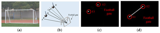
Figure 1.
Football gate images. (a) optical image. (b) observation geometry. (c) synthetic aperture radar (SAR) image of aperture AB. (d) SAR image of aperture CD.
To recover the disappeared linear structures in SAR images, several types of techniques have been reported in the literature. The most popular technique found in the literature that can recover the linear structures of targets is multi-aspect SAR imaging. The multi-aspect SAR imaging methods designed to take advantage of the anisotropy of the scattering characteristics of targets. By coherent or incoherent processing, this technique can combine scattering characteristics of different observation angles to provide more information for anisotropic objects. As a typical coherent multi-aspect SAR imaging technique, the circular SAR processes the full-angle echoes inorder to obtain the complete scattering characteristics of the illuminated scene based on its unique track advantage [17]. However, the extremely special observation geometry of circular SAR makes it difficult to apply to most SAR systemsm, such as spaceborne SAR systems. Unlike circular SAR imaging, multi-aspect SAR image fusion is an incoherent multi-aspect imaging technique that makes full use of the information contained in multiple different images to form a new image [18,19]. The new image can describe the target or scene more accurately, comprehensively, and reliably. Unfortunately, the non-coherent processing methods, such as image fusion, have strict requirements on the distribution of observation angles. If the distribution of observation angles is not suitable, then the information will be lost. As indicated in [20], the main energy of a linear structure is only concentrated on an extremely narrow angle, i.e., the normal angle. The linear structure can be completely imaged only when the radar sweeps over the normal direction of the structure. Otherwise, the linear structures completely disappear, except for its endpoints in the SAR image. Take the football image that is shown in Figure 1 as an example, if the data of the aperture AB are collected whereas the data of the aperture CD are neglected, then it is impossible to preserve the linear structure of the crossbar in the fused image. In addition to multi-aspect SAR imaging, a new feature enhancement approach for linear structures has attracted the attention of researchers working in the field of the restoration of SAR images. This approach can extract the anisotropic characteristics of scattered points in the wide-angle SAR image that is based on the iterative re-weighted Tikhonov regularization (IRWTR) [21]. Afterwards, the incomplete linear structures of the illuminated targets are restored based on the extracted anisotropic scattering behaviours. Unfortunately, this approach needs wide-angle SAR data, which may not be satisfied in some cases.
In this paper, we propose a linear structures recovery method for a SAR image based on spatial phase distribution feature. This method has the ability to identify the endpoints of the linear structures from the scattered points in SAR image via two side-observations and reconstruct linear structures that are based on the parametric scattering model. The main process of the proposed method can be divided into three steps. The first one is to classify the endpoints and scattered points in SAR image. It is achieved by setting a threshold related to the spatial phase distribution feature of endpoints. The spatial phase distribution feature is discovered through the parametric scattering model and it is a novel feature of endpoints that can effectively describe the essential difference between the endpoints of linear structures and isolated point targets. The second step is to determine which two endpoints can be formed into a linear structure. It is achieved by using the phase characteristics between two endpoints that belong to the same linear structure. At last, after estimating the parameters of the scattering model, the linear structures are reconstructed by adding the model-based echoes into the original radar echoes. The performance of the proposed method is also discussed in the aspect of complexity and robustness to noise. First, the dependence of complexity on the number of scattered points (formed by either point targets or linear structures) is discussed. Second, the performance of the proposed method under different levels of additive white Gaussian noises and speckle noises is discussed.
The remainder of this paper is organized, as follows. Section 2 describes the anisotropic phenomenon and scattering model of the linear structures. In Section 3, the main idea of the proposed linear structures reconstruction method is presented. In Section 4, the performance of the proposed reconstruction method for linear structures under different levels of noise corruption is presented. To evaluate the effectiveness and robustness of the proposed method, extensive microwave anechoic chamber experiment, tower crane radar experiment, and unmanned vehicle radar experiment are conducted in Section 5. Conclusions are drawn in Section 6 with some further discussions.
2. Problem Statement
2.1. Anisotropy of Linear Structures
As a basic geometric configuration, linear structure is an important component of vehicle, aircraft, railings and other targets. Unlike isotropic targets, the scattering feature of linear structure in SAR images is highly varying in different observation angles. To illustrate this anisotropic phenomenon, the backscattered data of a metal rob with different observation angles are simulated by CST. Figure 2 shows the observation geometry and corresponding imaging result. The main energy of a linear structure is only concentrated on an extremely narrow angle, i.e., the normal angle. The linear structure can be completely imaged only when the radar sweeps over the normal direction of it. Otherwise, the linear structure of target become two scattered points, which are at the end of the linear structure. Consequently, the linear structures and point targets are easily confused. This anisotropic phenomenon will visually degrade the appearance of SAR images.
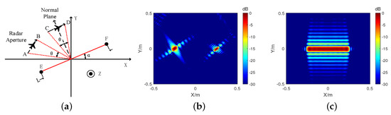
Figure 2.
Observation geometry and imaging result of a linear structure. (a) The observation geometry of Radar aperture AB and CD; (b) Imaging result of aperture AB; and, (c) Imaging result of aperture CD.
2.2. Scattering Models
SAR is an active acquisition instrument that generates radiation and captures signals backscattered from the illuminated scene [22]. For extended target, the resolution cell contains several scatterers, and none of which yield a reflected signal that is much stronger than the others, shown in Figure 3. In addition, these scatterers are uniformly distributed.
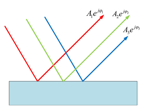
Figure 3.
The scattering model for an extended target.
With the assumptions of far-field and plane-wave propagation, the high-frequency radar backscattering features of a linear structure of extended target, as shown in Figure 4a, can be well modelled as incoherent sum of several backscattered waves, as follows [23,24,25,26,27]:
where c is the speed of light; is the reflection coefficient; is the azimuth time; represents the frequency range where denotes the carrier frequency; and, B denotes the bandwidth. The slant range represents the distance between the center of linear structure and the radar platform at azimuth time ; This integral formula (1) can be simplified to (2):
where is the azimuth angle of the radar; are the central positions of the linear structure; is the complex-valued amplitude of the linear structure related to length L, reflection coefficient and the unknown initial phase of the linear structure ; and, the R is the slant range between the center of the linear structure and radar platform. It can be described as:
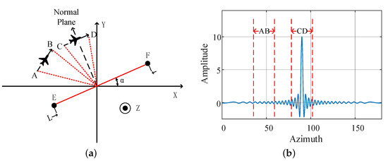
Figure 4.
Observation geometry and the echoes of a linear structure in azimuth time range frequency domain. (a) The observation geometry of a linear structure with length L and orientation . (b) The echoes of a linear structure in azimuth time range frequency domain and it can be described as a sinc function. The red lines are the azimuth boundaries of the radar apertures AB and CD.
The scattering feature of a linear structure is highly varying under different observation angles, as shown in Figure 2. This anisotropic feature can be described as a Sinc function along azimuth in range frequency domain according to (2), as shown in Figure 4b. The received echoes are on the main lobe of the Sinc function, when the radar passes through the normal plane of the linear structure. In this case, the linear structure can be completely imaged, as shown in Figure 2c. Otherwise, the received radar echoes are on the sidelobes of the Sinc function. In this case, the SAR image of the linear structure always appears as two isolated scattered points at the end of the linear structure, as shown in Figure 2b;
Assume that there is a linear structure located at . The coordinates of the endpoints E and F are and . The length and orientation of the linear structure is L and . The echo of point E and F can be expressed, as follows:
where is the reflection coefficient of point E and F; denotes the initial phase of the point scatterers; Additionally, , represent the slant range between the radar platform and point E and F. This formula can be simplified, as follows:
where denotes a complex-valued amplitude; By comparing, it is obvious that (5) is similar to the sidelobes of (2). This is the reason that the echoes of linear structure are so similar to the two-point target echoes when the radar does not sweep over the normal plane of the linear structure.
3. Linear Structures Recovery Method
3.1. Target Classification
Because the echo of a linear structure can be described by the scattering model, the phase feature in image domain can be obtained. Moreover, this feature can be utilized to classify the linear structures and point targets [28,29,30]. The BP algorithm deals with the time-domain signal after pulse compression. This algorithm can basically be understood as the coherent superposition of radar echo and the echo of an ideal point scatterer on the imaging grid. The value on the imaging grid can be expressed as:
where is the received radar echo; R is the slant range between the imaging grid and radar platform; is the azimuth time; represents the frequency range where denotes the carrier frequency; and, B denotes the bandwidth.
Assume that there is an isolated ideal point scatterer located on with reflection coefficient and unknown initial phase . The radar echo at azimuth time can be described, as follows:
By substituting (7) into (6), the peak value of the point scatterer in image domain is:
where is a constant. According to (7), is a complex number independent of the radar observation angle, as shown in Figure 5.
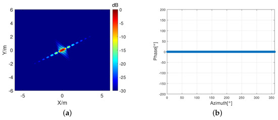
Figure 5.
The phase feature and SAR image of a point target. (a) SAR image of a point target. (b) The phase feature extracted from image under different observation angle.
Assume that there is a linear structure that is located on with length L, orientation reflection coefficient and unknown initial phase . The azimuth angle of radar is . The endpoints of the linear structure are point E and point F, and their coordinates are and . The coordinates of these two endpoints should comply with the following equation:
The parametric scattering model of this linear structure can be obtained by (2):
By substituting (10) into (6), the peak value of the endpoints E and F in image domain is:
where is a constant; denotes the carrier frequency; B denotes the bandwidth; represents the azimuth of radar; and, represents the orientation of the linear structure. Equation (11) shows that the peak value of the endpoint is a complex number and its imaginary part is closely related to the azimuth of radar and the orientation of the linear structure. When the the azimuth of radar changes, the imaginary part of the peak value may changes from a positive number to a negative one, which causes the phase of the complex number to mutate a lot. Moreover, there is a mutation in the phase when the radar platform passes through the normal plane of the linear structure, as shown in Figure 6. In Figure 6c, the red line represents the phase of endpoint E measured at aperture AB. In Figure 6d, the red line represents the phase of endpoint E measured at aperture CD. The spatial phase distribution feature of endpoints in image domain is different from the isolated point scatterers obviously by when comparing Figure 5 with Figure 6. Moreover, the phase difference between endpoint E and endpoint F is according to (11).
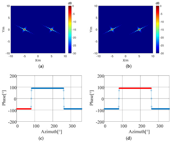
Figure 6.
The proposed spatial phase distribution feature in image domain. (a) SAR image of aperture AB. (b) SAR image of aperture CD. (c) The phase feature of endpoint E in aperture AB. The red line represents the phase of endpoint E measured at aperture AB. (d) The phase feature of endpoint E in aperture CD. The red line represents the phase of endpoint E measured at aperture CD.
Because the phase of endpoints change abruptly along the azimuth of radar, an identification algorithm of a endpoints and point targets is proposed using a spatial phase distribution feature. Figure 7 shows the location of radar platform and observed scene. It is worth noting that aperture AB and aperture CD should be located on the left and right sides of the linear structure normal plane. According to Figure 7b, the SAR image of aperture AB and aperture CD can be obtained by BP algorithm obviously. Based on and , the phase and amplitude of scattered points can be extracted, as follows:
where i is the index number of the scattered points in image and ; represent the coordinates of the target; means to extract the phase; and, means to extract the amplitude of scattered points. The spatial phase distribution in image and can be obtained by
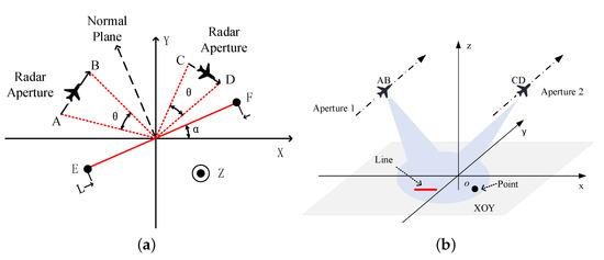
Figure 7.
The observation geometry where aperture AB and aperture CD should lay on the left and right sides of the linear structure normal plane. (a) The observation geometry. (b) The illuminated scene.
The endpoints and the ordinary point targets can be identified by comparing their spatial phase distribution feature with a threshold, as follows
where is the threshold; Equation (14) indicates that, if the is greater than the threshold , the scattered points in SAR images are endpoints. Otherwise, the scattered points are point targets. Because there are always some estimation errors under the noisy condition, and the phase is uniformly distributed within , the threshold is generally set to . After the above steps, the set of point targets and the set of endpoints can be classified. The detailed procedure of the endpoints and isolated point targets identification algorithm is illustrated as in Algorithm 1.
| Algorithm 1 Target Identification Method |
| Input: Received radar echoes and . |
| 1: Obtain images and by BP imaging algorithm. |
| 2: Estimate coordinates of the scattered points from and . The set of all scattered points are . Extract phase and of point from and . |
| 3: for do |
| 4: Compute the phase mutation values of point-like target . . |
| 5: If , the point-like target is a endpoint. Otherwise, it is a isolated point scatterer. |
| 6: end for |
| Output: The set of endpoints . |
3.2. Linear Structures Recognition
Next, the linear structures recognition algorithm is proposed to determine which two endpoints can be formed into a linear structure [31,32,33]. Let be the set of endpoints that belongs to linear structure and linear structure . Let , , , be the phase of endpoints, respectively. Obviously, there are six cases to form linear structures: (1) EF, (2) EG, (3) EH, (4) FG, (5) FH, and (6) GH. Because the phase difference between two endpoints that belong to the same linear structure is according to (11), we can set the threshold as . Case 1, 3, 4, and 6 must comply with this conditions whereas case 2 and case 5 can be excluded. In case 1, 3, 4, and 6, case 1 and 6 are true, while others are false Case 3 and 4 can be excluded according to relevant operation, as follows
where is the linear structure echo generated by scattering models based on the estimated parameters of endpoints; denote the complex conjugate; represents the received radar echo; denotes correlation of the -th case to form a linear structure; and, is the threshold. The detailed procedure of the linear structures recognition algorithm is illustrated as in Algorithm 2.
| Algorithm 2 Linear Structures Recognition Algorithm |
| Input: The set of endpoints . |
| 1: for do |
| 2: for do |
| 3: if then |
| 4: Compute by substituting , into (18), (19) and (20) |
| 5: Compute according to (2) |
| 6: Compute and by substituting into (15) and (16) |
| 7: If , and can form a linear structure. Otherwise, it is discarded |
| 8: end if |
| 9: end for |
| 10: end for |
| Output: The set of linear structure . |
3.3. Linear Structures Reconstruction
Since all of the scattered points in SAR images have been identified based on the spatial phase feature, the parameters of the linear structure can be roughly estimated based on the coordinates of the scattered points. Moreover, the disappeared linear structure scattering feature can be reconstructed based the parametric scattering model of linear structure in the previous section [34,35,36,37,38,39,40,41,42,43]. In this paper, we suppose that the illuminated scene of interest only contains point scatterers and linear structures. Some linear structures are only presented as two endpoints in the SAR image due to the observation angle. Suppose that the n-th endpoint and the m-th endpoint in the set of endpoints are judged as two endpoints of linear structure , the parameter set of can be presented as , according to (2). A rough estimation for can be obtained by
where and are the coordinates corresponding to the peak amplitudes of the m-th and n-th endpoints in the SAR image, respectively.
Next, the linear structure can be recovered based on the estimated scattering model [44]. Additionally, the parameter f is the frequency range; is the estimated length of the linear structure; is the azimuth time; is the estimated orientation of the linear structure; and, is a designed virtual azimuth angle of radar platform that passes through the normal plane of the linear structure. By adding the established virtual SAR image into the real SAR image of radar platform, the disappeared linear structure scattering feature can be reconstructed. Hence, by repeating the above steps, all of the disappeared linear structures can be reconstructed. At last, the procedure of proposed linear structures reconstruction method is summarized in Algorithm 3 for clarity.
| Algorithm 3 Linear Structures Reconstruction Method |
| Input: The set of linear structure and received radar echoes and . |
| 1: Obtain images and by BP imaging algorithm. |
| 2: Compute linear structures echoes based on the scattering models for the set of linear structure . |
| 3: Obtain virtual SAR images by BP imaging algorithm based on the . |
| Output: The Reconstructed SAR image is . |
4. Performance Analyses
4.1. Complexity Analysis of Linear Structures Recognition
Assume that there are N scattered points in the SAR image. The cases of connection between the endpoints is a permutation and combination problem. The number of all cases can be expressed as:
In the case of the raising number of the scattered points N, the number of cases to be judged will swiftly increase, which will bring a great calculation complexity. If the characteristics of two end points that belong to the same linear structure with a phase difference of 180 degrees are taken into account, the number of cases that need to be judged will become half of the original.
Although this can reduce the number of cases that need to be judged to some extent, the problem is still an exponential distribution. If the prior information of the target size is taken into account, that is, for a certain endpoint, only the other endpoints within a certain scale are considered, the total number of judgments required will drop sharply. In this case, the problem becomes a linear distribution, which can reduce the computational complexity to a certain extent. Figure 8 shows the simulation results.
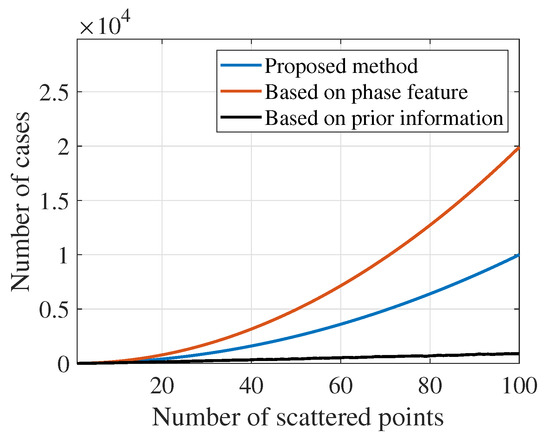
Figure 8.
The relationship between the number of scattered points and the numberof cases that need to be judged.
4.2. Robustness to Noise
There are lots of noises in real-world scenarios from the environment, radar system, and others. Therefore, the robustness to noise is also a highly desired requirement of the proposed method. To test the performance of the proposed method under noise corruption, different types and levels of noises are added to the echoes according to the preset signal-to-noise ratio (SNR), defined as follows.
where denotes strongest pixel of the original SAR image and is the variance of AWGN. In order to assess the performance of the phase mutation feature, we define the relative error (RE) of the phase, as
where K is the number of runs; is the phase extracted from images; and, is the truth value. Based on the Bayes decision rule, we adopt the minimum probability of error to describe the accuracy of the proposed method.
where is the conditional probability denotes that the probability of deciding when is true; is the prior probability. Assume that and represent the case of linear structure and point scatterers, respectively. The prior probability and are both equal to 0.5. The probability of error can be described, as follows
where N denotes the number of the simulation experiments; represents the number of deciding i when j is true in the entire experiments. We set under different SNRs in the following part.
First, to analyse the relationship between probability of error and additive noises, different levels of additive white Gaussian noises (AWGN) are added to the echoes and the performances are plotted in Figure 9. It is obvious that, with the SNR increasing, the and the relative error continuously decrease. When the SNR is lower than 18 dB, the reaches 0.4 and the relative error rise significantly, which indicates that linear structures and point targets are difficult to distinguish in this case. When SNR reaches 25 dB, the Pe drops to near 0 significantly, which means that, as long as the SNR is greater than 25 dB, the linear structures and points scatterers can be easily identified.
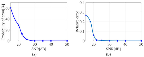
Figure 9.
Performance under different levels of AWGN. (a) Relationship between and SNRs. (b) Relationship between relative error and SNRs.
The value of the SAR image is modulated by the real RCS of objects by a multiplicative speckle noise. Next, different levels of speckle noises are added to the echoes to evaluate the relationship between probability of error and multiplicative noises. The stained SAR image can be described as
where I is the SAR image; X is the real RCS of objects in the illuminated scene; and, n is uniformly distributed random noise with mean 0 and variance V. The equivalent number of looks (ENL) can effectively measure the speckle noise level of the SAR image. The ENL of an intensity image is defined as
where is defined as
where denote the mean of the number. The symbol x is the intensity value of a large area in SAR image. Figure 10 shows the relationship between probability of error and multiplicative speckle noises. The result reveals that the speckle noise does not have a large impact on the error probability and the phase when SNR is higher than 20 dB.
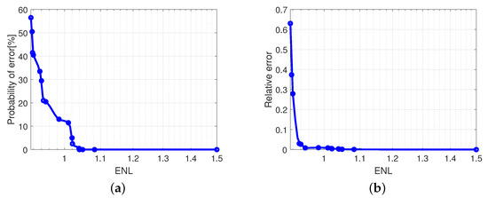
Figure 10.
Performance under different levels of speckle noises. (a) Relationship between and ENL. (b) Relationship between relative error and ENL.
5. Experimental Results
5.1. Computer Simulation
Several linear structures and isolated points targets are placed in the illuminated scene in order to verify the effectiveness of the proposed linear structures reconstruction method, and their parameter sets are shown in Table 1. In addition, the peak amplitudes of the SAR images from the linear structure and points are set equal to eliminate the influence caused by amplitudes. The corresponding radar parameters are listed in Table 2, where the two sub apertures located on the left and right sides of the linear structure normal plane, respectively. The received radar echoes from linear structures and isolated point scatterers are generated by (2). and the corresponding SAR images and obtained from the left-sided and right-sided apertures are shown in Figure 11. The results clearly show that the disappearance of linear structure AB and linear structures CD when the radar platform miss the normal plane of the lines and it is difficult to identify the scattered points. Table 3 shows the coordinates and phase of the scattered points extracted from images and .

Table 1.
Targets parameters.
Table 2.
Radar parameters.
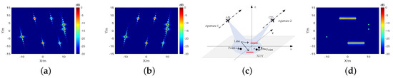
Figure 11.
Simulation results. (a) SAR image of left-sided aperture. (b) SAR image of right-sided aperture. (c) The observation geometry of the computer simulations. (d) The reconstructed SAR image based on scattering models.
Table 3.
Estimation results of the scattered points.
By comparing the spatial phase distribution feature with threshold rad, point A, B, C, and D are identified as endpoints, point E, F, and G are identified as point scatterers. Obviously, there are three cases to form linear structures: (1) AB, CD; (2) AC, BD; and, (3) AD, BC. Because the phase difference between two endpoints of the same linear structure is according to (11), case 3 is excluded. The can be obtained by (15), (16) and (17): , , , , , , , . By setting th threshold as , case 2 can be excluded and the case 1 is the final identification result. Based on (2) and the estimation result according to (18)∼(20), the virtual echoes and images can be generated. After adding the virtual images into the image , the reconstructed SAR image can be obtained, as shown in Figure 11d.
Furthermore, when considering the experiments at a lower signal-to-noise (SNR) ratio, the Gaussian noise with specific variance is added into the received echoes. The SNRs indicates the ratio of the peak power of the signal to the noise power in the CBP SAR images. The SNRs in the images is about 26 dB, and the corresponding imaging results have been deteriorated significantly when compared with Figure 11, as shown in Figure 12. The reconstructed results show that the 26-dB SNR does not have a significant impact on the identification and reconstruction of the targets.
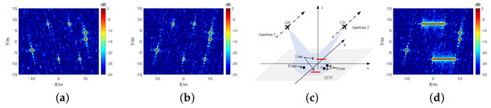
Figure 12.
Simulation results at SNR ≈ 26 dB. (a) SAR image of left-sided aperture. (b) SAR image of right-sided aperture. (c) The observation geometry of the computer simulations. (d) The reconstructed SAR image based on scattering models.
5.2. Real Data Experiments
5.2.1. Microwave Anechoic Chamber Experiment
As a preliminary verification, the effectiveness of the spatial phase distribution feature of the endpoints of linear structure is first examined in a microwave anechoic chamber. A metal cylinder and two metal spheres are placed on a foam column, respectively, as shown in Figure 13. The metal cylinder represents the linear structure, while the metal spheres represent the point scatterers. To simulate the rotation of the radar platform, the foam column and targets are placed on a two-dimensional turntable. The distance between the two same spheres approximately equals the length of the cylinder, and the length and radius of the metal cylinder are m and m. There is an absorbing material wall between the antenna and the foam column to eliminate the influence of the foam column. Figure 13c shows the observation geometry. The distances from the transmitting antenna and receiving antenna to the target center are 9.17 m and 9.33 m, respectively, and the angle between the transmitter and receiver is . Table 4 shows the radar parameters.
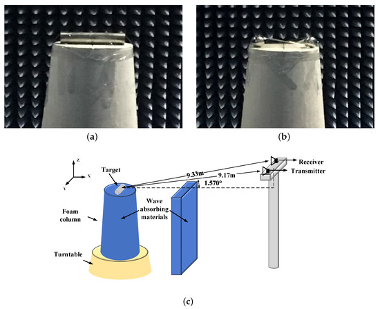
Figure 13.
The optical image of the illuminated targets. (a) The metal cylinder represents linear structure scatterers. (b) The metal spheres represent point scatterers. (c) The observation geometry in microwave anechoic chamber.
Table 4.
Radar parameters.
The corresponding imaging results are shown in Figure 14. Figure 14a,b show the CBP image of cylinder from the left-sided and right-sided observation, respectively. Figure 14c,d show the CBP image of spheres from the left-sided and right-sided observation, respectively. In these images, we can see that the CBP SAR images of cylinder and spheres are both strong points that are easily confused. However, there is still some difference between the real data and computer simulations. The target in the middle of two isolated points in Figure 14 might be clutter caused by the foam column. The spatial phase distribution of endpoints extracted from Figure 14a,b are rad and rad. The spatial phase distribution of spheres extracted from Figure 14c,d are rad and rad. Based on the phase mutation feature, the spheres and the endpoints of cylinder can be correctly identified by setting the threshold rad.
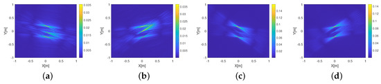
Figure 14.
The imaging results of the metal cylinder and spheres in the microwave anechoic chamber. (a) Image of cylinder at the left-sided observation. (b) Image of cylinder at the right-sided observation. (c) Image of sphere at the left-sided observation. (d) Image of sphere at the right-sided observation.
Furthermore, the Gaussian white noise with a certain variance is added into the data to produce noise-polluted echoes. The corresponding imaging results show that the targets have been severely distorted in Figure 15. The spatial phase distribution of endpoints that are extracted from Figure 15a,b are rad and rad. The spatial phase distribution of spheres extracted from Figure 15c,d are rad and rad. Based on the phase mutation feature, the spheres and the endpoints of cylinder can be correctly identified. Figure 16a shows the relationship between phase of spheres and SNRs and Figure 16b shows the relationship between phase of endpoints and SNRs. These results indicate that the phase feature of cylinder and spheres are not sensitive to noise. In Figure 16c, when SNRs dB, the will reach and below. The above experiment results demonstrate that the robustness of the phase mutation feature and verify that our proposed method can not only reconstruct the cylinder and spheres effectively, but also have a high success rate under the influences of noise.
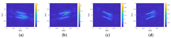
Figure 15.
The imaging results of the cylinder and spheres at SNR ≈ 26 dB in the microwave anechoic chamber. (a) Image of cylinder at the left-sided observation. (b) Image of cylinder at the right-sided observation. (c) Image of sphere at the left-sided observation. (d) Image of sphere at the right-sided observation.
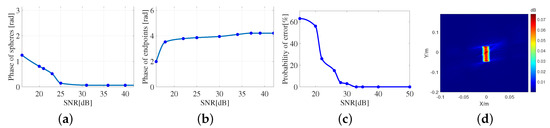
Figure 16.
The performance of proposed method. (a) Relationship between phase of spheres and SNRs. (b) Relationship between phase of endpoints and SNRs. (c) Relationship between and SNRs. (d) Reconstructed SAR image.
5.2.2. Tower Crane Radar Experiment
The tower crane radar experiment based on MIMO radar is conducted to further validate the performance of proposed method. The target observed in this experiment is a metal railing and multiple corner reflectors. Some absorbing materials are used to cover the pedestal in order to eliminate the influence of the pedestal on the scattering characteristics of the metal railing. In this experiment, the MIMO radar is mounted on the boom of a tower crane and the corresponding illuminated scene is shown in Figure 17. Table 5 shows the parameters of the MIMO radar.
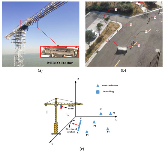
Figure 17.
The MIMO radar and the illuminated scene. (a) The MIMO radar. (b) The illuminated scene. (c) The observation geometry of the MIMO radar experiment.
Table 5.
Radar parameters.
There are five corner reflectors and a metal railing in the illuminated scene, as shown in Figure 17b. We use P1∼P5 to represent the five corner reflectors, and use E1 and E2 to represent the two endpoints of the metal railing in order to distinguish these scattered points in SAR images. To obtain the image of the metal railing under different observation, the metal railing is rotated along its center. Figure 18 shows the CBP images. These imaging results show that when the MIMO radar is on the normal plane of the metal railing, the entire metal railing can be imaged completely. However, when the MIMO radar is on the left side or right side of the normal plane, the linear structure scattering features disappears. This phenomenon proves the theory that is mentioned in the previous sections. Table 6 shows the phase mutation features extracted from the CBP images. The endpoints E1 and E2 are identified as endpoints of linear structure and P1∼P5 are identified as point scatterers, which matches the actual situation. The parameter set can be obtained by the coordinates of the endpoints: . Based on the parametric scattering model, the disappeared linear structure scattering feature can be reconstructed, as shown in Figure 18d.
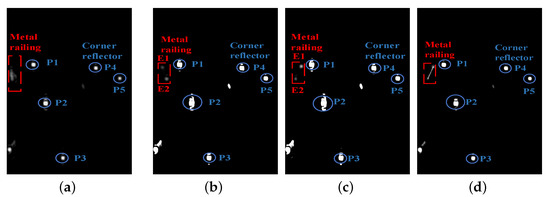
Figure 18.
The SAR image and reconstructed result of the tower crane radar experiment. (a) Observation on the normal plane, the entire metal railing can be imaged completely. (b) Observation on the left-side. (c) Observation on the right-side. (d) The reconstructed image.
Table 6.
Estimation results of the scattered points.
5.2.3. Unmanned Vehicle Radar Experiment
In this experiment, the MIMO radar is installed on a unmanned vehicle, and the illuminated targets are a football gate and multiple corner reflectors. The gate is rotated along its geometric center while the other corner reflectors were not moved in order to obtain the echoes for the football gate at multiple observation angles. In order to distinguish these scattered points in SAR images, we use P1∼P3 to represent the corner reflectors, and use E1 and E2 to represent the two endpoints of the football gate. Figure 19 shows the observation geometry and the CBP image. The phase mutation features extracted from the CBP images are shown in Table 7. It can be clearly seen that the linear structure scattering characteristics of the football gate disappear. By setting the threshold as 2 rad, the endpoints E1 and E2 are identified as endpoints of linear structure. The scattered points P1 and P3 are identified as point scatterers, which matches the actual situation. It is worth noting that the point target 2 is wrongly judged as the end point of the linear structure. However, the phase difference between the scattered points P2 and endpoint E1 or endpoint E2 cannot reach 180 degrees, so P2 and E1 or E2 cannot form a linear structures. Therefore, only E1 and E2 can form a linear structure. The scattering characteristics of the football gate can be reconstructed based on the parametric scattering model. Figure 20 shows the original BP image and reconstructed image.
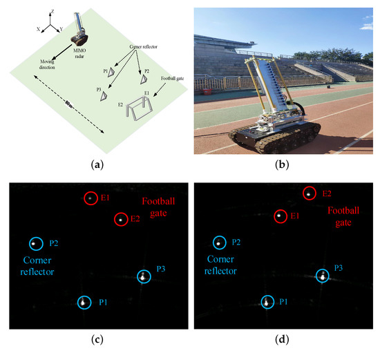
Figure 19.
The observation geometry and imaging results of the football gate. (a) The observation geometry. (b) The MIMO radar. (c) Observation on the left-side. (d) Observation on the right-side.
Table 7.
Estimation results of the scattered points.
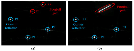
Figure 20.
The original BP image and reconstructed image of the football gate. (a) The original BP image. It can be clearly seen that the linear structure scattering characteristics of the football gate disappeared. (b) The reconstructed image of the football gate. The scattering characteristics of the football gate can be reconstructed.
6. Conclusions
This paper proposed a parametric SAR image recovery method for linear structures for distributed targets. The proposed method could efficiently distinguish the endpoints and isolated point targets via two side-observations and reconstruct the disappeared scattering features in SAR images. By extracting the spatial phase distribution feature in image domain, the proposed method is used to identify the endpoints among all of the scattered points and reconstruct the linear structures based on the parametric scattering model. The method can be generally divided into three procedures: endpoints and point targets classification, linear structures recognition, and linear structures reconstruction. The endpoints of linear structures and point targets are firstly identified by setting a threshold related to the spatial phase distribution feature. Subsequently, the spatial phase based linear structures recognition method is used to determine which two endpoints can be formed into a linear structure. The reconstructed images can be obtained by recovering the disappeared linear structure scattering features based on the parametric scattering models.
Computer simulations are first conducted to validate the effectiveness of the proposed method. Afterwards, three experiments, including microwave anechoic chamber experiment, tower crane radar experiment, and unmanned vehicle radar experiment, are conducted to further verify the effectiveness and robustness of the proposed method. The microwave anechoic chamber experiments examine the effectiveness of the spatial phase distribution feature. The results show that the spatial phase distribution feature in SAR image is a very discriminative feature for the recognition of linear structures and point targets. A further validation is performed based on tower crane radar experiment and unmanned vehicle radar experiment. The proposed method can reconstruct the disappeared linear structures with higher efficiency and effectiveness. The relative error of the proposed method is very low when SNR is higher than 28 dB, which demonstrates its superior effectiveness and robustness.
Future work will be focused on developing scattering characteristics of more types of targets to improve the universality of the proposed method.
Author Contributions
Conceptualization, Y.W. (Yuhan Wen), Y.W. (Yan Wang) and T.Z.; methodology, Y.W. (Yuhan Wen), Y.W. (Yan Wang) and X.C.; software, Y.W. (Yuhan Wen); validation, Y.W. (Yan Wang), X.C. and Z.D.; formal analysis, Y.W. (Yuhan Wen); investigation, Y.W. (Yuhan Wen) and X.C.; resources, Z.D. and T.Z.; data curation, Y.W. (Yuhan Wen); writing—original draft preparation, Y.W. (Yuhan Wen); writing—review and editing, Y.W. (Yan Wang); visualization, Y.W. (Yuhan Wen); supervision, Y.W. (Yan Wang) and X.C.; project administration, Y.W. (Yan Wang) and Z.D.; funding acquisition, Y.W. (Yan Wang) and T.Z. All authors have read and agreed to the published version of the manuscript.
Funding
This work was supported by the National science Fund for Distinguished Young Scholars (No. 61625103), the Beijing Natural Science Foundation (4202067), and by the Key Program of National Natural Science Foundation of China (No. 11833001, No.61931002).
Acknowledgments
The authors would like to thank the anonymous referees and the Associate Editor for useful comments that have helped to improve the presentation of this paper.
Conflicts of Interest
The authors declare no conflict of interest.
References
- Keller, J.B. A Geometrical Theory of Diffraction. Calc. Var. Appl. Proc. Symp. Appl. Math. 1958, 8, 27–52. [Google Scholar]
- Keller, J.B. Geometrical Theory of Diffraction. J. Opt. Soc. Am. 1962, 52, 116–130. [Google Scholar] [CrossRef]
- von Gioi, R.G.; Jakubowicz, J.; Morel, J.; Randall, G. LSD: A Fast Line Segment Detector with a False Detection Control. IEEE Trans. Pattern Anal. Mach. Intell. 2010, 32, 722–732. [Google Scholar] [CrossRef]
- Aggarwal, N.; Karl, W.C. Line detection in images through regularized hough transform. IEEE Trans. Image Process. 2006, 15, 582–591. [Google Scholar] [CrossRef]
- Argenti, F.; Lapini, A.; Bianchi, T.; Alparone, L. A Tutorial on Speckle Reduction in Synthetic Aperture Radar Images. IEEE Geosci. Remote Sens. Mag. 2013, 1, 6–35. [Google Scholar] [CrossRef]
- Fan, J.; Tomas, A. Target Reconstruction Based on Attributed Scattering Centers with Application to Robust SAR ATR. Remote Sens. 2018, 10, 655. [Google Scholar] [CrossRef]
- Lee, J.-S. Digital image enhancement and noise filtering by use of local statistics. IEEE Trans. Pattern Anal. Mach. Intell. 1980, PAMI-2, 165–168. [Google Scholar] [CrossRef]
- Frost, V.S.; Stiles, J.A.; Shanmugan, K.S.; Holtzman, J.C. A model for radar images and its application to adaptive digital filtering of multiplicative noise. IEEE Trans. Pattern Anal. Mach. Intell. 1982, PAMI-4, 57–166. [Google Scholar] [CrossRef] [PubMed]
- Kuan, D.T.; Sawchuk, A.A.; Strand, T.C.; Chavel, P. Adaptive noise smoothing filter for images with signal-dependent noise. IEEE Trans. Pattern Anal. Mach. Intell. 1985, PAMI-7, 165–177. [Google Scholar] [CrossRef] [PubMed]
- Lopès, A.; Nezry, E.; Touzi, R.; Laur, H. Maximum a posteriori speckle filtering and first order texture models in SAR images. In Proceedings of the 10th Annual International Symposium on Geoscience and Remote Sensing, College Park, MD, USA, 20–24 May 1990; pp. 2409–2412. [Google Scholar]
- Lopès, A.; Nezry, E.; Touzi, R.; Laur, H. Structure detection and statistical adaptive speckle filtering in SAR images. Int. J. Remote Sens. 1993, 14, 1735–1758. [Google Scholar] [CrossRef]
- Lee, J.-S. Digital image smoothing and the sigma filter. Comput. Vis. Graph Image Process. 1983, 24, 255–269. [Google Scholar] [CrossRef]
- Lee, J.-S. A simple speckle smoothing algorithm for synthetic aperture radar images. IEEE Trans. Syst. Man Cybern. 1983, SMC-13, 85–89. [Google Scholar] [CrossRef]
- Ding, B.; Wen, G.; Huang, X.; Ma, C.; Yang, X. Data Augmentation by Multilevel Reconstruction Using Attributed Scattering Center for SAR Target Recognition. IEEE Geosci. Remote Sens. Lett. 2017, 14, 979–983. [Google Scholar] [CrossRef]
- Ding, B.; Wen, G.; Huang, X.; Ma, C.; Yang, X. Target Recognition in Synthetic Aperture Radar Images via Matching of Attributed Scattering Centers. IEEE J. Sel. Topics Appl. Earth Observ. Remote Sens. 2017, 10, 3334–3347. [Google Scholar] [CrossRef]
- Samadi, S.; Çetin, M.; Masnadi-Shirazi, M.A. Multiple Feature-Enhanced SAR Imaging Using Sparsity in Combined Dictionaries. IEEE Geosci. Remote Sens. Lett. 2013, 10, 821–825. [Google Scholar] [CrossRef]
- Ishimaru, A.; Chan, T.-K.; Kuga, Y. An imaging technique using confocal circular synthetic aperture radar. IEEE Trans. Geosci. Remote Sens. 1998, 36, 1524–1530. [Google Scholar] [CrossRef]
- Zeng, T.; Ao, D.; Hu, C.; Zhang, K.; Zhang, T. Multi-angle BiSAR images enhancement and scatting characteristics analysis. In Proceedings of the 2014 International Radar Conference, Lille, France, 13–17 October 2014; pp. 1–5. [Google Scholar]
- Zeng, T.; Ao, D.; Hu, C.; Zhang, T.; Liu, F.; Tian, W.; Lin, K. Multiangle BSAR Imaging Based on BeiDou-2 Navigation Satellite System: Experiments and Preliminary Results. IEEE Trans. Geosci. Remote Sens. 2015, 53, 5760–5773. [Google Scholar] [CrossRef]
- Fan, Y.; Chen, X.; Wei, Y.; Ding, Z.; Wang, Y.; Wen, Y.; Tian, W. The Distributed SAR Imaging Method for Cylinder Target. In Proceedings of the IGARSS 2019–2019 IEEE International Geoscience and Remote Sensing Symposium, Yokohama, Japan, 28 July–2 August 2019; pp. 2921–2924. [Google Scholar]
- Gao, Y.; Xing, M.; Guo, L.; Zhang, Z. Extraction of Anisotropic Characteristics of Scattering Centers and Feature Enhancement in Wide-Angle SAR Imagery Based on the Iterative Re-Weighted Tikhonov Regularization. Remote Sens. 2018, 10, 2066. [Google Scholar] [CrossRef]
- Duan, H.; Zhang, L.; Fang, J.; Huang, L.; Li, H. Pattern-Coupled Sparse Bayesian Learning for Inverse Synthetic Aperture Radar Imaging. IEEE Signal Process. Lett. 2015, 22, 1995–1999. [Google Scholar] [CrossRef]
- Jackson, J.A.; Rigling, B.D.; Moses, R.L. Canonical Scattering Feature Models for 3D and Bistatic SAR. IEEE Trans. Aerosp. Electron. Syst. 2010, 46, 525–541. [Google Scholar] [CrossRef]
- Bhalla, R.; Ling, H.; Moore, J.; Andersh, D.J.; Lee, S.W.; Hughes, J. 3D scattering center representation of complex targets using the shooting and bouncing ray technique: A review. IEEE Antennas Propag. Mag. 1998, 40, 30–39. [Google Scholar] [CrossRef]
- Wright, J.; Yang, A.Y.; Ganesh, A.; Sastry, S.S.; Ma, Y. Robust Face Recognition via Sparse Representation. IEEE Trans. Pattern Anal. Mach. Intell. 2009, 31, 210–227. [Google Scholar] [CrossRef] [PubMed]
- Potter, L.C.; Moses, R.L. Attributed scattering centers for SAR ATR. IEEE Trans. Image Process. 1997, 6, 79–91. [Google Scholar] [CrossRef] [PubMed]
- Chiang, H.-C.; Moses, R.L.; Potter, L.C. Model-based classification of radar images. IEEE Trans. Inf. Theory 2000, 46, 1842–1854. [Google Scholar] [CrossRef]
- Liu, H.; Jiu, B.; Li, F.; Wang, Y. Attributed Scattering Center Extraction Algorithm Based on Sparse Representation with Dictionary Refinement. IEEE Trans. Antennas Propagat. 2017, 65, 2604–2614. [Google Scholar] [CrossRef]
- Cong, Y.; Chen, B.; Liu, H.; Jiu, B. Nonparametric Bayesian Attributed Scattering Center Extraction for Synthetic Aperture Radar Targets. IEEE Trans. Signal Process. 2016, 64, 4723–4736. [Google Scholar] [CrossRef]
- Jackson, J.A.; Moses, R.L. Synthetic Aperture Radar 3D Feature Extraction for Arbitrary Flight Paths. IEEE Trans. Aerosp. Electron. Syst. 2012, 48, 2065–2084. [Google Scholar] [CrossRef]
- Wei, Y.; Chen, X.; Fan, Y.; Ding, Z.; Wen, C. Analysis and identification of continuous line target in SAR echo based on sidelobe features. J. Eng. 2019, 2019, 5979–5981. [Google Scholar] [CrossRef]
- El-Darymli, K.; Gill, E.W.; Mcguire, P.; Power, D.; Moloney, C. Automatic Target Recognition in Synthetic Aperture Radar Imagery: A State-of-the-Art Review. IEEE Access 2016, 4, 6014–6058. [Google Scholar] [CrossRef]
- Yu, M.; Dong, G.; Fan, H.; Kuang, G. SAR Target Recognition via Local Sparse Representation of Multi-Manifold Regularized Low-Rank Approximation. Remote Sens. 2018, 10, 211. [Google Scholar]
- Dai, E.; Jin, Y.; Hamasaki, T.; Sato, M. Three-Dimensional Stereo Reconstruction of Buildings Using Polarimetric SAR Images Acquired in Opposite Directions. IEEE Geosci. Remote Sens. Lett. 2008, 5, 236–240. [Google Scholar]
- Rigling, B.D.; Moses, R.L. Three-dimensional surface reconstruction from multistatic SAR images. IEEE Trans. Image Process. 2005, 14, 1159–1171. [Google Scholar] [CrossRef] [PubMed]
- Xu, F.; Jin, Y. Automatic Reconstruction of Building Objects from Multiaspect Meter-Resolution SAR Images. IEEE Trans. Geosci. Remote Sens. 2007, 45, 2336–2353. [Google Scholar] [CrossRef]
- Xing, S.; Li, Y.; Dai, D.; Wang, X. Three-Dimensional Reconstruction of Man-Made Objects Using Polarimetric Tomographic SAR. IEEE Trans. Geosci. Remote Sens. 2013, 51, 3694–3705. [Google Scholar] [CrossRef]
- Ding, B.; Wen, G. Target Reconstruction Based on 3-D Scattering Center Model for Robust SAR ATR. IEEE Trans. Geosci. Remote Sens. 2018, 56, 3772–3785. [Google Scholar] [CrossRef]
- Zhu, X.X.; Shahzad, M. Facade Reconstruction Using Multiview Spaceborne TomoSAR Point Clouds. IEEE Trans. Geosci. Remote Sens. 2014, 52, 3541–3552. [Google Scholar] [CrossRef]
- Ertin, E.; Moses, R.L.; Potter, L.C. Interferometric methods for three-dimensional target reconstruction with multipass circular SAR. IET Radar Sonar Navigat. 2010, 4, 464–473. [Google Scholar] [CrossRef]
- Wu, J.; Liu, F.; Jiao, L.C.; Wang, X. Compressive Sensing SAR Image Reconstruction Based on Bayesian Framework and Evolutionary Computation. IEEE Trans. Image Process. 2011, 20, 1904–1911. [Google Scholar] [CrossRef]
- Ponce, O.; Prats-Iraola, P.; Scheiber, R.; Reigber, A.; Moreira, A.; Aguilera, E. Polarimetric 3-D Reconstruction From Multicircular SAR at P-Band. IEEE Geosci. Remote Sens. Lett. 2014, 11, 803–807. [Google Scholar] [CrossRef]
- Feng, D.; Chen, W. Structure Filling and Matching for Three-Dimensional Reconstruction of Buildings from Single High-Resolution SAR Image. IEEE Geosci. Remote Sens. Lett. 2016, 13, 752–756. [Google Scholar] [CrossRef]
- Gerry, M.J.; Potter, L.C.; Gupta, I.J.; van der Merwe, A. A parametric model for synthetic aperture radar measurements. IEEE Trans. Antennas Propagat. 1999, 47, 1179–1188. [Google Scholar] [CrossRef]


© 2020 by the authors. Licensee MDPI, Basel, Switzerland. This article is an open access article distributed under the terms and conditions of the Creative Commons Attribution (CC BY) license (http://creativecommons.org/licenses/by/4.0/).