Mapping Benthic Habitats by Extending Non-Negative Matrix Factorization to Address the Water Column and Seabed Adjacency Effects

Abstract

Monitoring of coastal areas by remote sensing is an important issue. The interest of using an unmixing method to determine the seabed composition from hyperspectral aerial images of coastal areas is investigated. Unmixing provides both seabed abundances and endmember reflectances. A sub-surface mixing model is presented, based on a recently proposed oceanic radiative transfer model that accounts for seabed adjacency effects in the water column. Two original non-negative matrix factorization ($NMF$)-based unmixing algorithms, referred to as $WADJUM$ (Water ADJacency UnMixing) and $WUM$ (Water UnMixing, no adjacency effects) are developed, assuming as known the water column bio-optical properties. Simulations show that $WADJUM$ algorithm achieves performance close to that of the $NMF$-based unmixing of the seabed without any water column, up to 10 m depth. $WUM$ performance is lower and decreases with the depth. The robustness of the algorithms when using erroneous information about the water column bio-optical properties is evaluated. The results show that the abundance estimation is more reliable using $WADJUM$ approach. $WADJUM$ is applied to real data acquired along the French coast; the derived abundance maps of the benthic habitats are discussed and compared to the maps obtained using a fixed spectral library and a least-square ($LS$) estimation of the seabed mixing coefficients. The results show the relevance of the $WADJUM$ algorithm for the local analysis of the benthic habitats.

1. Introduction

Remote measurement of benthic reflectance addresses a range of compelling environmental challenges, such as monitoring coral reefs [1], seagrass [2], or invasive seaweed [3], which serve key roles for coastal populations and the global environment. Coastal and inland waters are generally complex environments, whose remotely sensed reflectance may be highly variable due to simultaneous changes in bathymetry, water quality, seabed type, water surface and atmospheric conditions. In shallow waters, the decoupling of these effects has been shown to be more accurate when using hyperspectral data instead of multispectral data [4,5,6]. This is because a higher number of spectral bands, as well as an increased spectral resolution, allow reducing confounding effects between optically active parameters, e.g., by detecting the subtle changes in reflectance that originate from narrow absorption regions potentially present in seabed albedo [7,8]. Therefore, hyperspectral airborne remote sensing has been widely used for mapping water composition and bathymetry [9,10]. In coastal environments, hyperspectral remote-sensing methods that allow the simultaneous retrieval of bathymetry, water quality and benthic cover are often based on the inversion of a radiative transfer model that describes how light propagates into the water [11]. Semi-analytic parametric models [12,13], as well as numerical models such as Hydrolight [14], or more recently, the $OSOAA$ open source radiative transfer model [15], have been developed to describe the relationship between the seabed reflectance and remote-sensing reflectance by taking into account water attenuation. These models usually consider that four parameters affect the water-leaving radiance in addition to the water molecules: seabed depth and concentrations of three optically active constituents, namely chlorophyll ($Chl$), suspended non-algal particles ($SM$), and colored dissolved organic matter ($CDOM$) [16]. A classical approach could rely on estimating the parameters of the model, which provide the water column constituents (concentrations of chlorophyll, suspended matter, dissolved organic matter , and bathymetry). The retrieval of the bio-optical properties of the water column using an inversion algorithm is generally obtained using either look-up tables, iterative least-square (LS) [16], Maximum Likelihood (ML) [17,18], or Maximum A Posteriori (MAP) optimization [19,20].

In shallow water, the water column constituents estimation requires knowledge of the seabed reflectance spectrum. Generally, due to the spatial resolution of airborne or space sensors and to the complexity and variability of coastal areas, the seabed pixel reflectance is supposed to be a linear combination of endmember spectra.

When the seabed reflectance is not known but the endmember spectra are available, the coefficients of the linear mixing can be additionally estimated through the inversion process [21]. In the case when a sum-to-unity constraint is applied to the coefficients of the linear mixture, they represent the percentages of each spectrum in the considered pixel reflectance, also called abundance fractions (or abundances). This makes it possible to obtain abundance maps which provide understandable and clear information about the seabed composition. When only the shape of the endmember spectra is available, unknown scale factors are also necessary to provide the true endmember spectra. Then the mixing coefficients may depend both on those unknown scale factors as well as on the proportions of the materials, so the sum-to-unity constraint should not be applied, the estimation thus providing only coefficients maps for which the interpretation is not straightforward. Although the spectral library might not represent properly all the pure materials, it could be sufficiently comprehensive to be used as a basis. Then, the mixing coefficients may still be used to estimate the seabed spectrum. Note, however, that the coefficients derived for the latter case do not provide maps that are representative of the benthic species distribution.

When a spectral library is not available or not sufficiently representative of the benthic species, it is necessary to estimate both the mixing coefficients, and additionally the endmember signatures. Here, a difference is made between unsupervised unmixing, which we refer to estimating both mixing coefficients (abundances if the sum-to-unity constraint is applied), and endmember spectra in each observed pixel, and coefficient estimation, which we refer to estimating only the mixing coefficients, using a spectral library. Actually, due to natural variability, existing spectral libraries may not realistically represent the pure materials for a given observation, thus leading to erroneous abundance estimation. Interestingly, the non-negative matrix factorization ($NMF$) class of methods, broadcasted by Lee and Seung in the seminal articles [22,23], and extensively developed in [24], makes it possible to estimate both abundances and endmembers. Furthermore, such a method has shown to be able to adapt to various mixing models [25,26]. As an example, the case of multiple reflections between endmembers has been recently addressed using $NMF$ [27,28,29]. The consideration of the inter-pixel variability also remains a challenge for the community, and it has been addressed using unmixing methods [30,31,32].

In the case of seabed analysis, the influence of the water column needs to be included in the mixing model. Generally, the water constituents and the bathymetry are estimated. In [33], J. Goodman et al. introduced mixing coefficient estimation for seabed, using an adapted version of Lee’s parametric semi-analytical model [12,21,34], and linear mixing for seabed reflectance, using a known spectral library. They successively perform Lee’s inversion and estimate the seabed spectra mixing coefficients, in an algorithm called $LIGU$. A variant of $LIGU$ is also used in the $ZyCIAT$ toolbox by [35]. Seabed mapping is also developed in [36]. In [37], Maritorena’s radiative transfer model [13] has been used to combine iteratively $ML$ estimation and $NMF$ unmixing to obtain simultaneously the water parameters, the endmember spectra and the relative abundances. Recently a Bayesian approach has been proposed [20] for linear mixtures to jointly estimate the seabed reflectance and water optical properties while flexibly incorporating varied domain knowledge and in situ measurements, using Maritorena’s model, and simulations from Hydrolight radiative transfer code. A brief review of seabed analysis methods can be found in [38].

The adjacency effects represent the contamination of the radiance of a given target by photons scattered by the surrounding environment of this target. Most of the previous studies dealing with the adjacency effects in ocean color remote sensing, aimed at analyzing the influences of the atmosphere and/or of the neighboring land pixels on the radiance measured by a satellite sensor [39,40,41,42]. In [43], the authors propose an Alternating Direction Method of Multipliers ($ADMM$)-based unmixing method that takes into account adjacency effects in the atmosphere. Authors [44] have investigated the detection of adjacency effects in the ground implying water areas, as being a general unmixing problem, using several $NMF$-based methods. In [45], the focus is made for the first time on the analysis of the influence of the seabed adjacency effects; an analytical formulation of the radiative transfer equation is developed that includes the adjacency effects. The radiative transfer model developed in [45] has been used in a previous work [46], to introduce the new specific $NMF$-based unmixing method that is developed here.

The objectives of this paper are (i) to propose two sub-surface mixing models, either accounting for the adjacency effects or not, (ii) to develop two adapted $NMF$-based unmixing methods, in accordance with these models, iii) to analyze and quantify the efficiency of the proposed methods, by evaluating the impact of the adjacency effects on the results, and iv) to obtain abundance maps of the seabed from airborne hyperspectral images of a coastal area and assess their relevance.

To reach these objectives, the analytical formulation of the radiative transfer into the water column, recently proposed in [45], is taken into account as the original complete model, which is then adapted to the unmixing purpose. The adapted radiative transfer model and the mixed pixel decomposition are accounted for to derive a specific sub-surface mixing model. A new $NMF$-based unmixing method, hereafter referred to as $WADJUM$ (Water ADJacency UnMixing), is proposed. A simpler variant, referred to as $WUM$ (Water UnMixing) algorithm, which does not account for the adjacency effects induced by the seabed and the hydrosols present in the water column, is also presented. An analysis of the performance of the proposed unmixing methods is carried out by assessing the relative importance of the adjacency effects, and also the relative importance of the presence of a water column. Additionally, the impact of an error made on the water column composition is studied. Last, the $WADJUM$ algorithm is applied to real original data acquired on the coast of the Porquerolles Island, South of France. The resulting abundance maps are evaluated by comparison with a ground truth, and with coefficient maps that are obtained using an $LS$ coefficient estimation approach and a spectral library.

The paper is organized as follows: Section 2 is devoted to the theoretical developments. In Section 3, the unmixing performance is assessed by means of simulations that are performed using the $OSOAA$ open source radiative transfer model [15]. Section 4 provides results of the application of the proposed unmixing methods to real data, and Section 5 is devoted to a discussion.

2. Models and Methods

In this section, the underwater radiative transfer equation that was recently developed in [45] is briefly described. Such an analytic formulation has been established from the complete equation of the radiative transfer into the water column. This previous work has highlighted the influence of the adjacency effects induced by the seabed and by the hydrosols present in the water column.

The notations used in the paper are given in

Table 1. Notations used in the paper.

$\mathit{\delta }\uparrow$	Environment vector: contribution of the target pixel
	reflectance to diffuse upward radiance
$\delta$	Environment parameter, $\delta =mean(\delta \uparrow )$
${\mathbf{L}}_u$	Sub-surface upward radiance
${\mathbf{L}}_u^{dp}$	Radiance due to photons from the water column which have
	not interacted with the seabed
${\mathbf{L}}_{dir}$	Radiance due to photons directly transmitted by the water
	column after interaction with the seabed
${\mathbf{L}}_{dif}$	Radiance due to photons scattered after interaction with
	the seabed
${\mathbf{E}}_{tot}$	Incident downward flux that reaches the seabed
${\mathbf{E}}_{0-}$	Incident downward flux that reaches sub-surface level
${\mathbf{T}}_{dir}$	Direct upward transmittance of water column
${\mathbf{T}}_{dif}$	Diffuse upward transmittance of water column
${\mathit{\rho }}_t$	Reflectance of the target pixel
${\mathit{\rho }}_{env}$	Equivalent reflectance of the target pixel environment
	that contributes to the upward radiance, including the target
${\mathit{\rho }}_{adj}$	Equivalent reflectance of the pixels adjacent to the target
	that contributes to the upward radiance, not including the
	target
L	Number of wavelengths
I	Number of pixels in the whole image
J	Number of endmembers
${\mathbf{K}}_1$	Direct attenuation matrix of upward light for the whole
	image, with size $L\times I$
${\mathbf{K}}_2$	Diffuse attenuation matrix of upward light for the whole
	image, with size $L\times I$
${\mathbf{k}}_1$	Direct attenuation vector for one pixel
${\mathbf{k}}_2$	Diffuse attenuation vector for one pixel
$\mathbf{R}$	Matrix of observed sub-surface reflectance, with size $L\times I$
$\tilde{\mathbf{R}}$	Matrix $\mathbf{R}$ minus the water reflectance
$\mathbf{S}$	matrix containing endmember spectra, with size $L\times J$
$\mathbf{A}$	matrix containing abundance coefficients, with size $J\times I$
z	seabed depth(bathymetry), in m

.

2.1. Radiative Transfer Equation that Makes the Adjacency Effects Explicit

This work follows an in-depth analysis of various sources of photons that contribute to the sub-surface upward radiance radiative transfer phenomena within the water column, presented in [45]. From this paper, a schematic representation of the upward radiances corresponding to direct, diffuse, and water-leaving radiance is shown in Figure 1a. Let us note that the direct sun reflection on the water surface does not appear in this schematic representation, since aerial measurements are commonly acquired out of the sunglint geometry; at worse, the sunglint radiance contribution could be corrected from the data using dedicated sunglint correction algorithms [47].

The environment of the target pixel P of the seabed (for example, adjacent pixel M) contributes to the observed sub-surface radiance, due to the scattering of the light within the water column. Then, the total contributing seabed reflectance is not only associated with the target pixel, but also with its neighbors.

The observed sub-surface (depth $z=0-$) total upward radiance can be expressed as the sum of three main terms (Figure 1a):

$${\mathbf{L}}_u(P,0-)={\mathbf{L}}_{dir}(P,0-)+{\mathbf{L}}_{dif}(P,0-)+{\mathbf{L}}_u^{dp}(P,0-).$$

(1)

${\mathbf{L}}_u^{dp}$ is the radiance due to the upward photons that have not interacted with the seabed. Following the previous work in [45], the upward radiances ${\mathbf{L}}_{dir}$ and ${\mathbf{L}}_{dif}$ are both related to the downward flux, to the seabed reflectance and to the water column transmittance:

$${\mathbf{L}}_u(P,0-)=\frac{{\mathbf{E}}_{tot}\left(P\right)}{\pi }\odot {\mathbf{T}}_{dir}(0-)\odot {\mathit{\rho }}_t+\frac{{\mathbf{E}}_{tot}\left(P\right)}{\pi }\odot {\mathbf{T}}_{dif}(0-)\odot {\mathit{\rho }}_{env}+{\mathbf{L}}_u^{dp}(P,0-).$$

(2)

The symbol ⊙ denotes the elementwise product and each bold term corresponds to a spectral vector. ${\mathit{\rho }}_t$ and ${\mathit{\rho }}_{env}$ respectively refer to the target (pixel P) reflectance and the environment (P and adjacent pixels) reflectance.

2.2. Downward Flux ${\mathbf{E}}_{tot}$

The total incident downward flux that reaches the pixel P, ${\mathbf{E}}_{tot}\left(P\right)$, is the sum of four components, corresponding respectively to the direct, diffuse, coupling and reflected light (see Figure 1a):

$${\mathbf{E}}_{tot}={\mathbf{E}}_{dir}+{\mathbf{E}}_{dif}+{\mathbf{E}}_{coup}+{\mathbf{E}}_{ref}.$$

(3)

The coupling term ${\mathbf{E}}_{coup}$ depends on multiple reflections between the seabed and the water column. It therefore depends on the reflectance of the seabed environment, including the reflectance of the target pixel, through multiple products of seabed reflectances. To evaluate the importance of this non-linear effect in reflectance, a test case has been simulated, composed of 2400 various linear mixtures of four endmember spectra that are contained in the spectral library used for the experiments (shown in Section 3, Figure 5f, dotted spectra). The mixtures are representative of the spectral variability of seabed areas in the Porquerolles Alicaster Bay (Var, France). The objective is to evaluate the amount of variability of ${\mathbf{E}}_{tot}$ due to the multiple reflections between the seabed and the water column, described by the coupling term ${\mathbf{E}}_{coup}$. A variability index, defined as the maximum ratio over the wavelengths between the standard deviation and the mean value of the 2400 pixels reflectance, is found as $maxr\left(\mathbf{R}\right)=61\%$ for the seabed. The value of ${\mathbf{E}}_{tot}$ has been generated using $OSOAA$ model, including all the multiple reflections, for each pixel position and for three cases. The water quality is defined by the concentrations of the main optical constituents: chlorophyll-a, suspended matter, and colored dissolved organic matter. The clear water condition is defined as [$Chl=0.03{\mathrm{mg}·\mathrm{m}}^{-3},SM=0.01{\mathrm{mg}·\mathrm{L}}^{-1},CDOM=0.01{\mathrm{m}}^{-1}$], and the moderately turbid is defined as [$Chl=1{\mathrm{mg}·\mathrm{m}}^{-3}$, $SM=1{\mathrm{mg}·\mathrm{L}}^{-1}$, $CDOM=0.1{\mathrm{m}}^{-1}$]. The three considered cases are $c_1$: clear water, seabed depth $z=1\mathrm{m}$, $c_2$: moderately turbid water, $z=1\mathrm{m}$ and $c_3$: moderately turbid water, $z=10\mathrm{m}$. For each case, the standard deviation and the mean value of ${\mathbf{E}}_{tot}$ over the 2400 pixels have been calculated, and the resulting variability index, $maxr\left({\mathbf{E}}_{tot}\right)$, is reported in

Table 2. Maximum relative spread of the total downward radiance ${\mathbf{E}}_{tot}$ at the seabed level, due to the variability of the seabed reflectance and coupling illumination.

Water Column Condition	${\mathit{c}}_1$	${\mathit{c}}_2$	${\mathit{c}}_3$
$maxr\left({\mathbf{E}}_{tot}\right)$	$1.3\%$	$1\%$	$0.4\%$

.

The coupling term has the highest influence in the case of clear water and low depth. Out of all cases considered, a variability index of $61\%$ for the spectra of the seabed corresponds to a maximum variability index of $1.3\%$. Consequently, in the remainder of the paper, it is considered that the variation of ${\mathbf{E}}_{tot}$ with the seabed composition can be assimilated to (weak) noise. Then multiple reflections that cause the variations of ${\mathbf{E}}_{tot}$ can be neglected in the expression of the radiative transfer model of Equation (2). In the following of the paper ${\mathbf{E}}_{tot}$ is assumed to depend only on the water column bio-optical properties (bathymetry and turbidity), not on the seabed reflectance, so multiple products of seabed reflectances do not appear in the model.

2.3. Environment Function and Environment Reflectance Analysis

In [45], the authors make use of the environment function ${\mathbf{G}}_{env}$, as given in [42], also called $\delta \uparrow$. The environment function determines at each wavelength the weight of the target contributing to the upward diffuse radiance, relatively to its neighborhood. Typically, a value of one means that the target P contributes at $100\%$ to the sub-surface upward radiance; in other words, there is no adjacency effect from the neighborhood of the target for such a case. The environment function ${\mathbf{G}}_{env}$ depends on the size of the target, on the optical thickness of the water layer, and on the wavelength. It is lower for smaller targets, for a high number of scattering events of hydrosols, and for deep waters. For more details the reader is encouraged to refer to [45]. Here the notation $\delta \uparrow$ denotes its vectorial representation over the wavelengths, hereafter referred to as the ’environment vector’, which is plotted in Figure 1b for the case of moderately turbid water, a target pixel radius of 0.5 m, and various seabed depths. The variations of $\delta \uparrow$ with the wavelength are very smooth. In consequence it is assumed in the following that the spectral vector $\delta \uparrow$ can be replaced by its mean value over the wavelength domain, $\delta =\frac{1}{L}{\sum }_{\lambda =1}^L\delta \uparrow \left(\lambda \right)$, so-called the environment parameter. Please note that $\delta$, which provides the global contribution of the target pixel to the diffuse light in the range of 400 nm–700 nm, is approximately 72% for 5 m depth, whereas it is only 55% at 10 m, thus meaning that the adjacent pixels contribute 28% and 45% respectively to the diffuse light in these cases. Consequently, the contribution of pixels adjacent to the target pixel cannot be neglected in the diffuse sub-surface upward radiance.

Following [45], the equivalent environment reflectance of the seabed target pixel is developed as:

$${\mathit{\rho }}_{env}=\delta {\mathit{\rho }}_t+(1-\delta ){\mathit{\rho }}_{adj},$$

(4)

where ${\mathit{\rho }}_t$ is the target reflectance and ${\mathit{\rho }}_{adj}$ is the reflectance of the pixels adjacent to the target. To build the underwater mixing model, it is necessary to decompose ${\mathit{\rho }}_t$ and ${\mathit{\rho }}_{env}$ as mixtures of endmember spectra.

2.4. Decomposition of Target and Environment Reflectances

In this study, the assumption of linear mixing is made for the seabed sub-pixel decomposition. This is justified by the following considerations.

(i) The linear mixing model is currently used for seabed estimation with other methods (such as $LS$ inversion with a spectral library) [9,18,20,21,33,35,36,37,38,46].

(ii) As mentioned previously in Section 2.2, $OSOAA$ simulations have shown that non-linear interactions such as multiple reflections between the seabed and the water column do not significantly modify the downward flux ${\mathbf{E}}_{tot}$, and consequently the upward fluxes at the sea surface level. This is due to the water attenuation. At the sub-surface level, simulations showed that the only notable bottom interaction with the water column is the adjacency effect resulting from the scattering of photons by the water column, at the order one, given by the term ${\mathbf{L}}_{dif}$ shown in Figure 1a.

To consider a whole image instead of a single target pixel ${\mathit{\rho }}_t$, the target pixel index i is now introduced in the notation, for all the concerned variables. The target pixel reflectance is decomposed as :

$${\mathit{\rho }}_i=\sum _{j=1}^J{\mathbf{s}}_j{a}_{j,i}=\mathbf{S}{\mathbf{a}}_i,$$

(5)

where $a_{j,i}$ is the abundance fraction of the pure material (endmember) reflectance ${\mathbf{s}}_j$ in the target pixel i, and J is the number of endmembers. $\mathbf{S}$ is composed of the endmember spectra arranged in columns, and the vector ${\mathbf{a}}_i$ holds the abundances of each endmember in pixel i.

The approximation of a limited number of influencing neighboring pixels is relevant in this investigation. For the sake of clarity, the model is developed with a neighborhood given by the N nearest pixels (usually $N=4$ or $N=8$) and could be easily generalized to a wider neighborhood. Then ${\mathit{\rho }}_{adj}=\frac{1}{N}{\sum }_{n\in {\mathcal{V}}_t,n\ne t}{\mathit{\rho }}_n$, where ${\mathit{\rho }}_n$ is the reflectance of pixel n, in the neighborhood $\{{\mathcal{V}}_t,n\ne t\}$ of the target pixel.

Following Equation (4), the equivalent environment reflectance corresponding to a target pixel i of the sub-surface image is defined as:

$${\mathit{\rho }}_{env,i}={\delta }_i\sum _{j=1}^J{a}_{j,i}{\mathbf{s}}_j+(1-{\delta }_i)\frac{1}{N}\sum _{n\in {\mathcal{V}}_i,n\ne i}\sum _{j=1}^J{a}_{j,n}{\mathbf{s}}_j=\sum _{j=1}^J\left[\sum _{n\in {\mathcal{V}}_i}{p}_{n,i}{a}_{j,n}\right]{\mathbf{s}}_j=\mathbf{S}\mathbf{A}{\mathbf{p}}_i.$$

(6)

The coefficient $p_{n,i}$ is $p_{n,i}=\frac{1-{\delta }_i}{N}$ if $n\in {\mathcal{V}}_i,n\ne i$, $p_{n,i}={\delta }_i$ if $n=i$, and else $p_{n,i}=0$. $\mathbf{S}$ is the $L\times J$ matrix containing all the endmembers arranged in columns, $\mathbf{A}$ is the $J\times I$ abundance matrix, each of its rows corresponding to an endmember, and the $I\times 1$ vector ${\mathbf{p}}_i$ contains the coefficients $p_{n,i}$.

2.5. Sub-Surface Mixing Model Considering the Adjacency Effects

The last step to obtain the sub-surface mixing model consists of expressing the sub-surface reflectance as a function of the seabed endmembers spectra and abundances. The mixing model is derived from the radiative transfer equation (Equation (1)), jointly with the development of the environment reflectance proposed in Equation (6).

The contribution of the water column to the water upward radiance, namely ${\mathbf{L}}_u^{dp}$ (see Table 1 and Figure 1a), is subtracted from Equation (2), and the equation is divided by the downward illumination at surface level ${\mathbf{E}}_{0-}$ in order to obtain reflectance values (here the division ⊘ is elementwise). Equation (7) is obtained as follows:

$$\begin{array}{c}\hfill \left[{\mathbf{L}}_u-{\mathbf{L}}_u^{dp}\right]\oslash {\mathbf{E}}_{0-}={\mathbf{E}}_{tot}\oslash \pi {\mathbf{E}}_{0-}\odot {\mathbf{T}}_{dir}\odot {\mathit{\rho }}_t+{\mathbf{E}}_{tot}\oslash \pi {\mathbf{E}}_{0-}\odot {\mathbf{T}}_{dif}\odot {\mathit{\rho }}_{env}.\end{array}$$

(7)

For each pixel i of the whole data, the following notations are introduced:

$$\begin{array}{cc}{\tilde{\mathbf{r}}}_i& =[{\mathbf{L}}_u-{\mathbf{L}}_u^{dp}]\oslash {\mathbf{E}}_{0-};\hfill \\ {\mathbf{k}}_{1,i}& =\left[{\mathbf{T}}_{dir}\odot {\mathbf{E}}_{tot}\right]\oslash \pi {\mathbf{E}}_{0-};{\mathbf{k}}_{2,i}=\left[{\mathbf{T}}_{dif}\odot {\mathbf{E}}_{tot}\right]\oslash \pi {\mathbf{E}}_{0-}.\hfill \end{array}$$

(8)

By using the mixture decomposition of ${\mathit{\rho }}_{env}$ and ${\mathit{\rho }}_t$, provided in Equation (6), the expression in (7) becomes:

$${\tilde{\mathbf{r}}}_i={\mathbf{k}}_1\odot \left(\mathbf{S}{\mathbf{a}}_i\right)+{\mathbf{k}}_2\odot \left(\mathbf{S}\mathbf{A}{\mathbf{p}}_i\right).$$

(9)

For the entire scene containing I pixels and L wavelengths, the proposed sub-surface mixing model, denoted as $S{M}_{wadj}$ in the following, is then:

$$\tilde{\mathbf{R}}={\mathbf{K}}_1\odot \left(\mathbf{S}\mathbf{A}\right)+{\mathbf{K}}_2\odot \left(\mathbf{S}\mathbf{A}\mathbf{P}\right).$$

(10)

The $L\times I$ matrices $\tilde{\mathbf{R}},{\mathbf{K}}_1,{\mathbf{K}}_2$ are constructed with all the spectral vectors arranged in columns, and the matrix $\mathbf{P}$, which depends on the environment parameter ${\delta }_i$ at each pixel, is an $I\times I$ matrix. The adjacency effects caused by the photons scattered by the water column are described by the additive term ${\mathbf{K}}_2\odot \left(\mathbf{S}\mathbf{A}\mathbf{P}\right)$ in Equation (10).

Let us note that if the adjacency effects are not taken into consideration (i.e., assuming $\delta =1$), the matrix $\mathbf{P}$ becomes the identity, $\mathbf{P}={\mathbf{Id}}_{I\times I}$, so the following simpler sub-surface mixing model, denoted as $S{M}_{wnoadj}$, is obtained:

$$\tilde{\mathbf{R}}=({\mathbf{K}}_1+{\mathbf{K}}_2)\odot \left(\mathbf{S}\mathbf{A}\right).$$

(11)

2.6. Unmixing Method

The objective of the unmixing method consists of estimating both matrices $\mathbf{A}$ and $\mathbf{S}$. Here, the case where the water column characteristics are assumed to be known is being considered, i.e., that ${\mathbf{K}}_1$ and ${\mathbf{K}}_2$ are known and do not need to be determined. Such a case could be realistic when bio-optical measurements of the water column (i.e., water quality) have been carried out and when the bathymetry data are available from other means, for example using LiDAR techniques. Water composition parameters could also be estimated by using an $LS$ inversion method that would not require the accurate knowledge of the seabed (for example $SWIM$ code [48]), or alternatively by inversion using a fixed spectral library [36].

Then ${\mathbf{E}}_{0-},{\mathbf{E}}_{tot},{\mathbf{L}}_u^{dp},{\mathbf{T}}_{dir},{\mathbf{T}}_{dif},\delta$ can be numerically calculated for each pixel, using the $OSOAA$ radiative transfer model, to obtain the matrices ${\mathbf{K}}_1,{\mathbf{K}}_2,\mathbf{P}$. The matrix $\mathbf{P}$ is beforehand calculated for a chosen neighborhood size, which should depend on the pixel size and the scattering properties of the water column.

To solve the joint estimation of abundances and endmembers problem, a cost function $RQE$, defined in Equation (12), is minimized.

$$RQE=\parallel {\tilde{\mathbf{R}}}_{obs}-\tilde{\mathbf{R}}{\parallel }_{Fro}^2.$$

(12)

The $RQE$ is the Frobenius norm of the difference between the observed sub-surface reflectance modified according to (8) (see also Table 1), ${\tilde{\mathbf{R}}}_{obs}$, and the estimated one, $\tilde{\mathbf{R}}$, given by the expression of Equation (10). $\tilde{\mathbf{R}}$ depends on the variable matrices $\mathbf{A}$ and $\mathbf{S}$.

Since the unmixing problem is ill-posed, solutions from local minima of the cost function may be obtained, or many global minima could exist, possibly giving erroneous endmembers and abundances. Initialization is then a key step for the unmixing procedure. The application of constraints allows the range of solutions to be reduced. Generally, constraints are chosen according to some characteristics of the data which are then guaranteed to be preserved [49,50]. Two variants of $NMF$ are developed hereafter, respectively so-called $WADJUM$, corresponding to the mixing model $S{M}_{wadj}$ expressed in Equation (10), and $WUM$, corresponding to the mixing model $S{M}_{wnoadj}$ of Equation (11). The two variants are both based on the $Minidisco$ algorithm [50], which uses an alternate projected gradient descent with an Armijo-Lin-based rule [24,51], and optional regularization, such as the sum-to-unity constraint ($STU$) for the abundances, or the minimum dispersion constraint for the spectra [50]. The estimation of the matrices $\mathbf{A},\mathbf{S}$ is obtained following Equation (13):

$$\begin{array}{c}\hfill [{\mathbf{A}}_{est},{\mathbf{S}}_{est}]={argmin}_{(\mathbf{A},\mathbf{S})}\left[RQE(\mathbf{A},\mathbf{S})+\Lambda (\mathbf{A},\mathbf{S})\right].\end{array}$$

(13)

$\Lambda$ denotes regularization terms that can be added to the $RQE$ criterion. In our experiments, a soft constraint to encourage the sum-to-unity for abundances is used, ${\Lambda }_{STU}={\lambda }_{STU}({\mathbf{I}}_{1J}\mathbf{A}-{\mathbf{I}}_{1I}){({\mathbf{I}}_{1J}\mathbf{A}-{\mathbf{I}}_{1I})}^T$. The vector ${\mathbf{I}}_{1J}$ is composed of the values ’one’; the regularization coefficient ${\lambda }_{STU}$ is empirically set to $0.5$ after various trials.

For the $WADJUM$ algorithm, the gradients of $RQE$, relative to $\mathbf{A}$ and $\mathbf{S}$, are detailed in Equation (14), where ${}^t$ denotes the transpose.

$$\begin{array}{c}\nabla RQ{E}_{\mathbf{S}}=\left[{\mathbf{K}}_1\odot \left({\tilde{\mathbf{R}}}_{obs}-{\mathbf{K}}_1\odot \left(\mathbf{S}\mathbf{A}\right)-{\mathbf{K}}_2\odot \left(\mathbf{S}\mathbf{A}\mathbf{P}\right)\right)\right]{\mathbf{A}}^t+{\mathbf{K}}_2\odot \left[\left({\tilde{\mathbf{R}}}_{obs}-{\mathbf{K}}_1\odot \left(\mathbf{S}\mathbf{A}\right)-{\mathbf{K}}_2\odot \left(\mathbf{S}\mathbf{A}\mathbf{P}\right)\right)\right]{\left(\mathbf{A}\mathbf{P}\right)}^t\\ \nabla RQ{E}_{\mathbf{A}}={\mathbf{S}}^t\left[{\mathbf{K}}_1\odot \left({\tilde{\mathbf{R}}}_{obs}-{\mathbf{K}}_1\odot \left(\mathbf{S}\mathbf{A}\right)-{\mathbf{K}}_2\odot \left(\mathbf{S}\mathbf{A}\mathbf{P}\right)\right)\right]+{\mathbf{S}}^t\left[{\mathbf{K}}_2\odot \left({\tilde{\mathbf{R}}}_{obs}-{\mathbf{K}}_1\odot \left(\mathbf{S}\mathbf{A}\right)-{\mathbf{K}}_2\odot \left(\mathbf{S}\mathbf{A}\mathbf{P}\right)\right)\right]{\mathbf{P}}^t.\end{array}$$

(14)

In the $WADJUM$ unmixing algorithm, updates of $\mathbf{A}$, $\mathbf{S}$, and $\tilde{\mathbf{R}}$ are successively performed at each iteration. The values of $\mathbf{S}$ and $\mathbf{A}$ are restricted to vary between 0 and 1, by setting the negative values to 0 and setting to 1 the values greater than 1. The optimization is stopped after 1000 iterations or after a threshold error is attained ($1\%$ of relative variation of $\tilde{\mathbf{R}}$).

An additive regularization term for the endmembers could also be used for example to minimize the spread of the endmembers (or the volume of the endmember simplex) as defined in [50]. However in the case of underwater unmixing, this constraint is not appropriate, due to the shape of the water column attenuation that strongly mitigates the signal between 600 nm and 700 nm (see Figure 2), resulting in possibly flat estimated spectra in this range if this constraint is applied.

Please note that the simpler variant of the underwater unmixing method for which no adjacency effects are taken into consideration, referred to as $WUM$, is obtained from the same algorithm, by setting $\mathbf{P}={\mathbf{Id}}_{I\times I}$.

3. Analysis of Performance Based on Simulations

Simulations are carried out to evaluate the performance of the proposed $WUM$ and $WADJUM$ algorithms.

3.1. Evaluation Metric

The results are evaluated using the mean spectral angle mapper (SAM) and the mean normalized $RMSE$, defined as follows in Equation (15):

$$\begin{array}{c}\hfill SAM=\frac{1}{N_{\omega }}\sum _{\omega }{\left[\frac{1}{I}\sum _i\left({cos}^{-1}\left(\frac{\left({\mathbf{s}}_i^t{\widehat{\mathbf{s}}}_i\right)}{\left(\sqrt{{\mathbf{s}}_i^t{\mathbf{s}}_i}\sqrt{{\widehat{\mathbf{s}}}_i^t{\widehat{\mathbf{s}}}_i}\right)}\right)\right)\right]}_{\omega };N{M}_{RMSE}=\frac{1}{N_{\omega }}\sum _{\omega }{\left(\frac{\parallel \mathbf{M}-\widehat{\mathbf{M}}{\parallel }_{Fro}}{{\parallel \mathbf{M}\parallel }_{Fro}}\right)}_{\omega }.\end{array}$$

(15)

Here $\omega$ and i respectively refer to the realizations (different noise generation and random initialization) and to the pixels, ${\mathbf{s}}_i$ and ${\widehat{\mathbf{s}}}_i$ refer to the true and estimated spectra, respectively; $\mathbf{M}$ and $\widehat{\mathbf{M}}$ refer to the true and estimated matrix, respectively. The generic matrix $\mathbf{M}$ can be $\mathbf{A}$, $\mathbf{S}$, ${\mathbf{K}}_1$, or ${\mathbf{K}}_2$. As the solution of the unmixing method is obtained up to a permutation for the matrices $\mathbf{A}$ and $\mathbf{S}$, the best match between true and estimated endmembers is performed before calculating the normalized $RMSE$.

The benchmark for evaluating the performance of the proposed algorithms is to apply the unmixing method on the seabed in the absence of a water column, in order to compare the proposed underwater unmixing algorithms with a method from the literature that considers both abundance and endmember estimation. The results of the two sub-surface unmixing algorithms $WUM$ and $WADJUM$ are compared to those of the simple unmixing of the seabed with no water column, using the algorithm $Minidisco$ [50], hereafter referred to as `$NMF$, no water’, using the same random initialization. This reference allows the testing of only the influence of the perturbation due to the water column, because the gradient-based optimization used is the same as the one of $WADJUM$ and $WUM$.

3.2. Simulated Data

The influence of the water column optical properties (attenuation due to scattering and absorption by hydrosols) is accounted for using $OSOAA$ model simulations, using the selected water turbidity and depth as inputs of $OSOAA$. Please note that the approximations outlined in Section 2 to establish the model given in Equation (10) were not applied on simulated data, since the radiative terms ${\mathbf{L}}_u^{dp},{\mathbf{E}}_{tot},{\mathbf{E}}_{0-}$, ${\mathbf{T}}_{dir},{\mathbf{T}}_{dif},\delta \uparrow$ were calculated using the $OSOAA$ radiative transfer model, including all multiple reflections on the seabed and the water column. Some stationary white noise was also added to the sub-surface reflectance $\tilde{\mathbf{R}}$ to simulate environment and sensor noise, with an SNR value of 40 dB. The values of ${\mathbf{K}}_1$ and ${\mathbf{K}}_2$ determine the relative importance of the direct and scattered light, respectively. 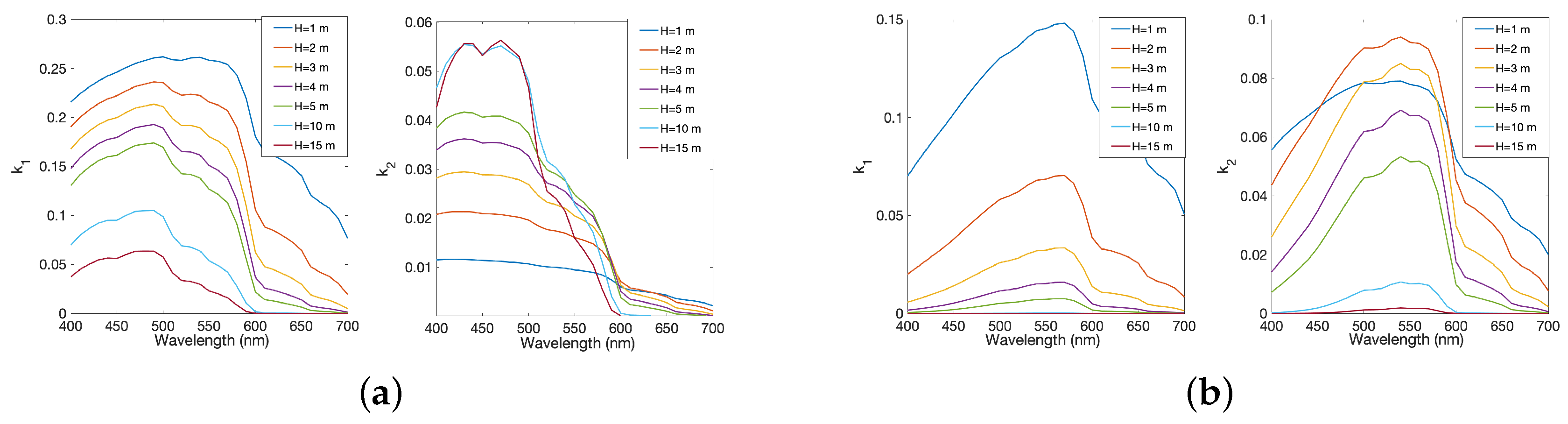Figure 2 shows the spectral variation of one column of the matrices ${\mathbf{K}}_1$ and ${\mathbf{K}}_2$ (respectively ${\mathbf{k}}_1$ and ${\mathbf{k}}_2$), corresponding to one pixel, for various depths ranging from 1 m to 15 m, and for two water turbidities (clear water, Figure 2a; moderately turbid water, Figure 2b).

The direct attenuation vector ${\mathbf{k}}_1$ always decreases with the depth whatever the wavelength, whereas the diffuse attenuation vector ${\mathbf{k}}_2$ shows a more complex behavior with depth. This is because the illumination ${\mathbf{E}}_{tot}$ at the seabed level and the direct transmittance ${\mathbf{T}}_{dir}$ both systematically decrease with depth, whereas the diffuse transmittance ${\mathbf{T}}_{dif}$ could either increase or decrease with depth, depending on the range of seabed depth and on the turbidity of the water. Therefore, the matrix ${\mathbf{K}}_2$ which is expressed as ${\mathbf{T}}_{dif}\odot {\mathbf{E}}_{tot}\oslash \pi {\mathbf{E}}_{0-}$, varies with depth following a compromise between depth and water turbidity. For very shallow water (e.g., seabed depth lower than 2 m), the direct attenuation term ${\mathbf{k}}_1$ contributes more than the diffuse attenuation term ${\mathbf{k}}_2$, so the influence of the adjacency effect induced by neighboring pixels may not be noticeable. However, in some cases, ${\mathbf{k}}_2$ is comparable to or even higher than ${\mathbf{k}}_1$, for example when the seabed depth z is greater than 10 m in clear water, and when z is greater than 2 m in the considered moderately turbid water. For those cases, the use of the model proposed in Equation (10)) for the unmixing is relevant because the adjacency effect has a significant impact on the total upward radiance.

Seabed reflectance data were generated using a random linear mixing of four endmember spectra representative of benthic species. These spectra were selected from a spectral library shown in Figure 5f (marked spectra) that had been measured during a field experiment that occurred in the Porquerolles Island, France, in September 2015. The measured spectra covered various types of seabed composition such as Caulerpa taxifolia algae, Posidonia seagrass, sand and substratum. They were sampled between 400 nm and 700 nm with a 10 nm step (31 wavelengths). The abundances were randomly generated using a maximum abundance of 85% for each endmember (no pure pixel), and some stationary white noise was added to the seabed image, in order to reach an SNR value of 40 dB at the seabed level. The hyperspectral image size is $(100\times 24)\mathrm{pixels}\times 31\mathrm{wavelengths}$.

3.3. Influence of the Consideration of the Adjacency Effects within a Seabed Unmixing Algorithm

The objective of this sub-section is to test the relevance of introducing the adjacency effects within the seabed unmixing method. To this end, a comparison is performed between the $WADJUM$ algorithm ($S{M}_{wadj}$ model), and the $WUM$ algorithm ($S{M}_{wnoadj}$ model). The unmixing method is also applied in the absence of a water column, using the $Minidisco$ algorithm [50], denoted as `$NMF$, no water’ in the figures. The results of $Minidisco$ serve as a benchmark for testing the influence of the water column on the unmixing results, using the same gradient-based optimization than the proposed NMF-based methods $WADJUM$ and $WUM$, without any influence of the water column.

The soft sum-to-unity constraint as defined in Section 2.6 is the only regularization process applied in the simulations, in order to avoid any interference with the evaluation of the influence of the adjacency effects on the unmixing algorithm.

The unmixing algorithm was initialized using biased endmembers, obtained using a random mixing of the true endmembers with other spectra from the spectral library shown in Figure 5f. Each initialization spectrum was composed of $80\%$ of the true endmember plus $20\%$ of a uniform random mixture of the true endmember and another one from the library. The abundances were then initialized using the $FCLS$ (Fully Constrained Least-Square) algorithm [52] applied to the seabed. The algorithms were developed in the $MATLAB$ language. $Minidisco$ ($NMF$, no water) converged in about 4 s on a standard laptop computer (Intel(R) Core(TM) i7-461, CPU $3.00$ GHz, 16 Mo RAM), whereas $WADJUM$ and $WUM$ running times were longer to attain the stopping condition (about 150 s). All the algorithms were initialized in the same manner.

Two water conditions were considered, clear water ($Chl$ = 0.03 mg·m${}^{-3}$, $SM$ = 0.01 mg·L${}^{-1}$, $CDOM$ = 0.01 m${}^{-1}$), and moderately turbid water ($Chl$ = 1 mg·m${}^{-3}$, $SM$ = 1 mg·L${}^{-1}$, $CDOM$ = 0.1 m${}^{-1}$). In very turbid water conditions, due to the water attenuation, the amount of information issued from the seabed is not sufficient to envisage blind unmixing application.

Figure 3 represents the spectral angle mapper value ($SAM$), the normalized root mean square error ($N{S}_{RMSE}$) on estimated endmember spectra, and the $N{A}_{RMSE}$ on estimated abundances, obtained for clear and moderately turbid waters, a pixel radius value of $0.5$ m and water depth z set to $[1,2,3,4,5,10]$ m. Each result is averaged over 10 realizations of noise and random initialization.

The results of the unmixing method using $Minidisco$, applied to the case where the water column is not present, show an angle error around $0.02$ rad, a normalized $RMSE$ around $3\%$ for the spectra, and around $10\%$ for the abundances. The presence of the water column expectedly degrades the performance of the unmixing methods. However, the range of errors remains acceptable for both algorithms; as an example, in the clear water case the angle error is around $0.03$ rad and the normalized $RMSE$ is around $6\%$ for spectra, and the $N{A}_{RMSE}$ is around $12\%$ for abundances. In clear water, the difference between $WUM$ and $WADJUM$ is not tremendous, because the direct term ${\mathbf{K}}_1$ is greater than the diffuse term ${\mathbf{K}}_2$, so the adjacency effect has small relative influence. In the case of moderately turbid water, the $WUM$ algorithm (no adjacency) gives very poor performance from z higher than 4 m, thus making this unmixing method not applicable (relative errors greater than $30\%$ for spectra and greater than $40\%$ for abundances), whereas the performance of $WADJUM$ remains about the same as the one obtained in clear water context. Standard deviations are comparable for the $WUM$ and $WADJUM$ algorithms in the case of clear water, whereas the $RMSE$ obtained using the $WUM$ algorithm appears to be unstable for moderately turbid waters at the intermediate seabed depth of 5 m. Therefore, the proposed $WADJUM$ algorithm allows efficient performance of the unmixing of the seabed with specifications close to those obtained when the unmixing is carried out in the absence of a water column. In moderately turbid water, it appears necessary that the unmixing method takes into consideration the adjacency effects to estimate the seabed endmembers and corresponding abundances.

3.4. Analysis of the Robustness of the Unmixing Methods with Respect to a Lack of Knowledge of the Water Column Properties

In the previous sections, ${\mathbf{K}}_1$ and ${\mathbf{K}}_2$ were supposed to be perfectly known. However, in real-world conditions, knowledge of the water attenuation is not perfect.

It is reminded here that the values of ${\mathbf{K}}_1,{\mathbf{K}}_2$ and $\delta$ (thus the matrix $\mathbf{P}$) depend both on the water quality, which is more or less homogeneous in small areas, and on the bathymetry, which could potentially vary from one pixel to another. To examine the impact of an error made on the water column optical properties, the true values of ${\mathbf{K}}_1$, ${\mathbf{K}}_2$ and $\delta$ are replaced by biased ones in the inputs of $WUM$ and $WADJUM$ algorithms. The way in which the errors on ${\mathbf{K}}_1,{\mathbf{K}}_2$ and $\delta$ are generated has a significant influence on the results. Although it is not possible to test all configurations, two cases are analyzed hereafter.

3.4.1. Error on the Bathymetry

Here the performance of the algorithms is evaluated when a random error on the bathymetry is applied, for two values of the true depth, $z_{true}=5.5$ m and $z_{true}=9.5$ m, in the case of moderately turbid water. The biased values of the bathymetry are obtained using a uniform random generation of the seabed depth, $\mathcal{U}[-0.5,0.5]$ m, centered on the true values. The corresponding biased values of ${\mathbf{K}}_1,{\mathbf{K}}_2$ and $\delta$, used for the input of the algorithms, are obtained by interpolating between the values given by $OSOAA$ simulations for $z=5$ m and $z=6$ m (resp. $z=9$ m and $z=10$ m). The performance of the unmixing methods is presented in

Table 3. Performance of $WUM$ and $WADJUM$ when a random error with an uniform law $\mathcal{U}[-0.5,0.5]$ m is added to the seabed depth, for a true seabed depth of $5.5$ m and of $9.5$ m, in the case of moderately turbid water.

True Depth	$\mathit{NK}{1}_{\mathit{RMSE}}$	$\mathit{NK}{2}_{\mathit{RMSE}}$	${\mathit{NS}}_{\mathit{RMSE}}$$\mathit{WUM}$	$\mathit{WADJUM}$	${\mathit{NA}}_{\mathit{RMSE}}$$\mathit{WUM}$	$\mathit{WADJUM}$
$5.5$ m	$6\%$	$5\%$	$22\%\pm 7\%$	$4\%\pm 1\%$	$30\%\pm 11\%$	$14\%\pm 2\%$
$9.5$ m	$48\%$	$18\%$	$41\%\pm 3\%$	$22\%\pm 7\%$	$60\%\pm 7\%$	$29\%\pm 12\%$

.

When $z_{true}=5.5$ m, the relative error on ${\mathbf{K}}_1$ and ${\mathbf{K}}_2$ due to the error on bathymetry is not very high ($NK{1}_{RMSE}=6\%$, $NK{2}_{RMSE}=5\%$). However the unmixing results remain satisfactory for $WADJUM$ only ($N{S}_{RMSE}=4\%$, $N{A}_{RMSE}=14\%$), whereas the $WUM$ algorithm provides unsatisfactory estimate for spectra ($N{S}_{RMSE}=22\%$) and for abundances ($N{A}_{RMSE}=30\%$).

For the deepest seabed case ($z_{true}=9.5$ m), the random error on the depth leads to a significant error on the attenuation matrices, $NK{1}_{RMSE}=47\%$ and $NK{2}_{RMSE}=18\%$. This high error on the water attenuation results in degraded performance for both $WUM$ ($N{S}_{RMSE}=41\%$, $N{A}_{RMSE}=60\%$) and $WADJUM$ ($N{S}_{RMSE}=22\%$, $N{A}_{RMSE}=29\%$), although the estimation remains better for $WADJUM$.

In any case, the $WADJUM$ algorithm still provides better results than the $WUM$ algorithm, so the relevance of taking in consideration the adjacency effects for the unmixing is confirmed. In moderately turbid water, the $WADJUM$ algorithm is robust to a uniform error of amplitude 1 m on the bathymetry at a depth of $5.5$ m, but this error has a greater impact at a depth of $9.5$ m, thus limiting the field of application of the unmixing method in the case of biased knowledge of the bathymetry.

3.4.2. Error on the Knowledge of the Water Quality

The objectives of this paragraph are (i) to study the consequences of a bias on the knowledge of water quality, (ii) to verify if scenes with constant bathymetry are easier to map than scene with varying bathymetry.

The test image contains five areas of each $100\times 24$ pixels and 31 spectral bands, each area corresponding to one fixed depth, respectively $z=1\mathrm{m},2\mathrm{m},3\mathrm{m},4\mathrm{m},5\mathrm{m}$. The results obtained by the $WUM$ and $WADJUM$ algorithms, applied to each constant depth area separately, are compared to those obtained when the unmixing method is applied to the entire image composed of all five areas. This makes it possible to evaluate the method both when the depth is not constant and when the depth is fixed. For the entire image, the estimation of abundances is obtained globally but evaluated in each area separately, whereas the estimation and evaluation of endmember spectra is only global. The true water quality is the moderately turbid one. The erroneous values of ${\mathbf{K}}_1,{\mathbf{K}}_2,\delta$ are generated by interpolating between their respective values obtained for clear and moderately turbid water with a fixed proportion (resp. $5\%$ and $95\%$), for each depth. The relative $RMSE$ errors between true and biased values of ${\mathbf{K}}_1,{\mathbf{K}}_2$ are presented in

Table 4. Normalized $RMSE$ between the true ${\mathbf{K}}_{1,true},{\mathbf{K}}_{2,true}$ and the biased ${\mathbf{K}}_1,{\mathbf{K}}_2$, due to an erroneous knowledge for water quality, for $z=[1,2,3,4,5]\mathrm{m}$, and moderately turbid water.

$\mathit{z}\left(\mathit{m}\right)$	1	2	3	4	5
$NK{1}_{RMSE}$	$5\%$	$14\%$	$32\%$	$68\%$	$138\%$
$NK{2}_{RMSE}$	$4\%$	$4\%$	$3\%$	$3\%$	$3\%$

.

It can be seen that the normalized error on the direct term, $NK{1}_{RMSE}$, becomes significant when the depth increases, while $NK{2}_{RMSE}$ does not vary much with the depth. The results are reported in Figure 4.

For the case of separate constant seabed depth areas, due to the increasing error on ${\mathbf{K}}_1$ in deepest parts, the error on the endmember spectra estimate, $N{S}_{RSME}$, also increases with depth, although it is lower using $WADJUM$ than $WUM$. The endmember spectra cannot be accurately retrieved due to the bias on water attenuation. The abundance estimate on the separate areas remains quite good for all the depths despite the distorted retrieval of the endmember spectra, as observed in Figure 4. This could be explained by the constant depth in one area, which results in the same distortion for all spectra, thus still corresponding to distinguishable classes of benthic species.

On the contrary, for the entire image, the error on endmember spectra estimate, $N{S}_{RSME}$, shows an intermediate value between the performance obtained at lower and higher bathymetries on the separate parts. To interpret this result, it should be reminded that the parts of the global image corresponding to the deepest areas have the smallest reflectance values, due to the attenuation induced by the water column, so these parts contribute more weakly to the $RQE$, which is the criterion that is optimized during the unmixing process. Therefore, the global optimization essentially involves the shallowest parts of the entire image. Thus, the global endmember estimate remains relatively good. For the entire image, the errors on abundances obtained using $WUM$ and $WADJUM$ both increase slightly on the shallowest part when using the global unmixing method; this could be due to the degradation of the global endmember estimates at $z=1$ m. $WADJUM$ is more performing than $WUM$ in the deepest parts.

In conclusion, a small variation in the water quality knowledge may lead to quite a large bias on ${\mathbf{K}}_1$ at the largest seabed depths. The endmember estimation degrades with this bias and is not reliable for a relative error of the water attenuation greater than $14\%$ . The abundance estimation is more robust, the error remains acceptable (maximum $13\%N{A}_{RMSE}$) when using $WADJUM$ in the case of biased water attenuation knowledge. The difference between $WADJUM$ and $WUM$ performance may be not significant for constant depth areas. The performance of the abundance estimates could deteriorate when observing scenes characterized by highly variable seabed depths.

4. Application to Real Data

An airborne data campaign has been conducted by the Hytech Imaging company [53] on 13 September 2017, using the $HySpex$ sensor [54], over the Porquerolles Island coast (France). The hyperspectral images were corrected to obtain georeferenced reflectance images. The pixel size of the observed images is 0.5 m × 0.5 m, the wavelengths have been resampled to achieve a 10 nm resolution, and the images were analyzed in the spectral range from 410 nm to 700 nm. Sun glint [47] and the air/water interface [22] were corrected to finally obtain the sub-surface remote-sensing reflectance image $\tilde{\mathbf{R}}$ (in sr${}^{-1}$) by subtracting the water upward reflectance. In situ measurements were performed with the help of the PNPC (Parc National de Port Cros) [55] at six stations in the Alicaster Bay, where the seabed depth ranges from 2 m to 20 m. In situ data consisted of measuring chlorophyll-a ($Chl$), suspended matter ($SM$) and colored dissolved organic matter ($CDOM$) concentrations. A diver brought back samples of the benthic species from the seabed to measure their spectral signatures (Figure 5d,f). A Remotely Operated underwater Vehicle (ROV) data campaign has been carried out by the French Institute for Marine Exploration (Ifremer) [56] over a transect of $1500\times 2$ m surface, with a high spatial resolution ($2.3$ cm), to acquire $RGB$ images at the seabed level [57]. The images have been classified in three classes, namely sand, Posidonia, and Caulerpa taxifolia. The supervised classification method is based on color information, using a weighted combination of Euclidian and spectral angle distance, and reference spectra representative of each class. This classification allows the generation of an abundance map of $0.5$ m spatial resolution, which serves as a ground truth data for the evaluation of the unmixing results. A colored composition of the sub-surface image, with the vehicle’s path, is shown in Figure 5a, together with the bathymetry and an example of $ROV$ underwater image containing sand, Posidonia and Caulerpa taxifolia (Figure 5b,c).

The mean measured values of the concentrations of the water constituents in the Alicaster Bay were $Chl$ = 0.03 mg·m${}^{-3}$, $SM$ = 0.5 mg·L${}^{-1}$, $CDOM$ = 0.05 m${}^{-1}$. The bathymetry was provided by the $LITTO3D$ database, available in [58], supported by the $IGN$ (French National Institute for Geographical and Forestry Information) and the $SHOM$ (Marine Hydrographic and Oceanographic Service). Please note that the entire French coast bathymetry is available with a precision of $95\%$, and 1 m spatial resolution. The values of the water attenuation ${\mathbf{K}}_1$ and ${\mathbf{K}}_2$, and $\delta$, have been calculated beforehand using the OSOAA radiative transfer model, the mean measured values of the concentrations of water constituents, $Chl,SM,CDOM$, and the bathymetry.

4.1. Initialization of the Unmixing

Initial matrices ${\mathbf{S}}_{init}$ and ${\mathbf{A}}_{init}$ must be determined for the unmixing procedure. In order to find such matrices, two steps are performed.

Step one: a first sea column correction is carried out from a classical $LS$ method (lsqcurvefit function of $MATLAB$), using a chosen library ${\mathbf{S}}_0$, and the model $S{M}_{wnoadj}$ of Equation (11), to obtain the coefficient matrix ${\mathbf{C}}_{est}$ . Although the spectra in ${\mathbf{S}}_0$ should be representative of the local benthic habitat, they are not supposed to be the exact endmembers. Consequently, the sum-to-unity constraint is ignored in the inversion, in order to permit scale factors for the spectra. A preliminary estimate of the seabed reflectance, given by ${\mathbf{X}}_{inv}={\mathbf{S}}_0*{\mathbf{C}}_{est}$, is then recovered.

Step two : the initial matrix ${\mathbf{S}}_{init}$ is obtained by applying the $VCA$ algorithm [59] to ${\mathbf{X}}_{inv}$, and the initial abundance matrix ${\mathbf{A}}_{init}$ is obtained using the $FCLS$ algorithm [52] and ${\mathbf{S}}_{init}$.

4.2. Experiments on the Validation Zone

The validation data have been divided in two parts, Part 1 and Part 2, as shown in Figure 5a, in order to avoid the use of big matrices for calculation. A spectral library has been acquired in the Porquerolles area in June 2016, September 2016 and September 2017. Different spectra representative of sand, substratum and Posidonia are shown in Figure 6.

It can be seen that the Posidonia class can be represented by various spectral signatures, as well as sand or substratum. Moreover, organic surface deposits such as waste stems can be found on dark sand and substratum, so their reflectances are very close to those of brown Posidonia or shell colonized Posidonia. Consequently, in large areas such as the one covered by the robot transect, some confusion can be expected between Posidonia and dark sand or substratum classes. In the following, only estimated abundances (${\mathbf{A}}_{est}$) and coefficients (${\mathbf{C}}_{est}$) are shown, the estimated spectra being distorted due to the approximative knowledge of the water attenuation.

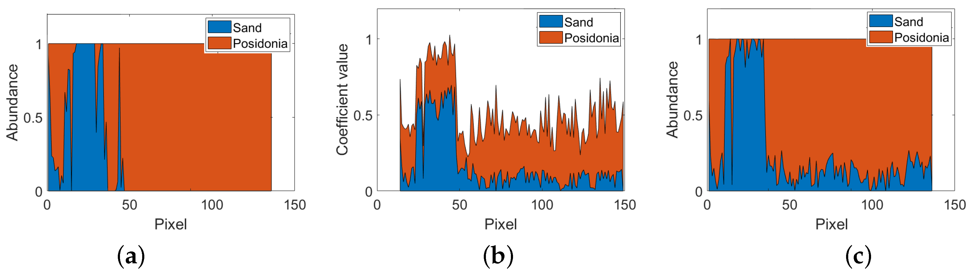
4.2.1. Abundance Estimation Performed on Part 1

In this area, only Posidonia seagrass and sand are present. We consider two reflectance spectra (green and brown) for the Posidonia class, and the clear sand spectrum for the sand, which is locally light and homogeneous (see Figure 6). The ground truth abundances ${\mathbf{A}}_{GT}$, the $LS$ estimated coefficients ${\mathbf{C}}_{est}$, and the $WADJUM$ estimated abundances ${\mathbf{A}}_{est}$ are respectively shown in Figure 7a–c, as a function of the pixel index. The abundances/coefficients of the two $Posidonia$ classes have been fused. The $N{A}_{RMSE}$ errors are calculated for the three unmixing methods: $VCA+FCLS$ performed on the reconstructed seabed ${\mathbf{X}}_{inv}$ with no water column, and $WUM$/$WADJUM$ performed on the sub-surface reflectance image $\tilde{\mathbf{R}}$.

It can be seen that for both $LS$ estimation and unmixing methods, some sand is detected where the ground truth indicates only Posidonia. This is due to the variability of the Posidonia reflectance, which can be colonized by shells, so with a spectral signature close to the sand’s one. The distributions of the abundances of the two classes estimated using $WADJUM$ better fit the ground truth than the $LS$ coefficients, which shows the interest of the unmixing method. The abundance errors obtained for the three unmixing methods are ${NA}_{RMSE}=22\%$ using $VCA+FCLS$ performed on ${\mathbf{X}}_{inv}$, ${NA}_{RMSE}=19\%$ using $WUM$ or $WADJUM$ performed on $\tilde{\mathbf{R}}$. As two classes are present, the error is the same for the sand and for the $Posidonia$. The error is not calculated for the coefficients ${\mathbf{C}}_{est}$, because they are not normalized.

4.2.2. Abundance Estimation Performed on Part 2

In the Part 2 of the validation area there is a $Caulerpa$ colonization surface, located in craters from ancient projectile testing. The bathymetry varies from 6 m to 14 m, and is around 10 m in the $Caulerpa$ location. As the monitoring of the $Caulerpa$ is an important issue for the PNPC, we focus on the estimation of such a benthic habitat. $Posidonia$ and sand/substratum are in the same class. Results are presented in Figure 8. Please note that the ground truth shows incomplete classification at pixel ca. 85 (Figure 8a).

The distribution of $Caulerpa$ given by the $LS$ coefficients ${\mathbf{C}}_{est}$ is more dispersed than the distribution given by ${\mathbf{A}}_{est}$, obtained using $WADJUM$. The difference between the initialization using $VCA+FCLS$ performed on ${\mathbf{X}}_{inv}$, and the output of $WUM$ and $WADJUM$ performed on $\tilde{\mathbf{R}}$, is not tremendous for the estimation of $Caulerpa$ abundance: $N{A}_{RMSE}=15\%$ using $VCA+FCLS$, $N{A}_{RMSE}=13\%$ using $WUM$, $N{A}_{RMSE}=12\%$ using $WADJUM$.

In conclusion, the validation shows a real improvement using an unmixing strategy instead of $LS$ coefficient estimation, and a slight improvement using $WUM$ or $WADJUM$ performed on the sub-surface images compared to the use of $VCA+FCLS$ performed on the reconstructed seabed with no water column. The difference between $WUM$ and $WADJUM$ performances is very low, according to the simulations results in clear water condition such as the clear water in Porquerolles area (see Section 3.3). Let note that both $VCA+FCLS$ and $WUM$ results should degrade in moderately turbid conditions, because these two methods do not take into account the adjacency effects. Furthermore, the water quality is not accurately known, further reducing the difference in performance between the $WUM$ and $WADJUM$ unmixing methods (see Section 3.4.2).

4.3. Experiment on Another Area

A small area of $200\times 530$ pixels (100 m × 265 m), delimited by a red rectangle in the Figure 5a, has been selected as shown in Figure 9b. This area shows a diversified seabed, and the bathymetry is in the range between 2 m and 6 m (Figure 9d). The endmembers used for the $LS$ inversion were dark green $Posidonia$, sand, substratum and photophilic algae, given in Figure 5f. Photophilic algae consist of a rich variety of algae conditioned by light penetration, often located on rocky areas. They constitute an important environmental issue. The environment parameter $\delta$, ${\mathbf{K}}_1,{\mathbf{K}}_2$ values and the water reflectance ${\mathbf{L}}_u^{dp}\oslash {\mathbf{E}}_{0-}$ were calculated in the same way as in Section 4.2. Because the size of the matrix $\mathbf{P}$ is too large for computation on $MATLAB$, the image has been split into five contiguous sub-images to run the $WADJUM$ algorithm, and the obtained abundances have been reassembled (Figure 9c). This presupposes the hypothesis of the same classes of pure materials being made for the five sub-images, and also that some variations in the spectra representative of one class could be permitted. Please note that the imperfect knowledge of the water column (i.e., the water quality) resulted in distorted endmember spectra as mentioned in Section 3 (not shown). As the substratum and brown $Posidonia$ Classes may overlap (see Section 4.2), a single class, denoted as Subs/Pos in Figure 9a,c is associated with both brown Posidonia and substratum classes.

The abundances estimated using $WADJUM$, as shown in Figure 9c, can be qualitatively evaluated by comparison with the sub-surface image (Figure 9b). The sand is correctly mapped. The green $Posidonia$ seagrass is observed in the middle of the area identified as substratum/brown $Posidonia$, and photophilic algae are located on the edge of the area of settlement of the $Posidonia$ and substratum. In conclusion, the qualitative examination of the seabed mapping indicates a distribution of the benthic habitat that is consistent with the observed sub-surface image.

The comparison between the coefficients given by ${\mathbf{C}}_{est}$ (Figure 9a) and the abundances obtained in ${\mathbf{A}}_{est}$ (Figure 9c), shows some differences in the spatial distribution of benthic habitat (apart from the scale, which is not the same for abundances and coefficients), circled in red. The green $Posidonia$ is erroneously detected on the seabed right corner of the coefficients in ${\mathbf{C}}_{est}$, and the substratum/brown $Posidonia$ could be confused with sand in ${\mathbf{C}}_{est}$.

5. Discussion

The first question addressed in this work is: is it relevant to perform seabed unmixing, due to attenuation by the water column?

An accurate model of the radiative transfer was necessary to overcome the low magnitude of the signal issued from the seabed at the sub-surface level. The $OSOAA$ model allowed us to select the radiative components from the complete equations of the radiative transfer inside the water column that were sufficiently impacting the sub-surface signal to be distinguished from noise. Although many non-linear interactions such as multiple reflections are present in the water column, an analysis of those contribution to the total bottom illumination showed that those non-linear phenomena do not significantly influence the upward radiance at the sub-surface level, for depths comprised between 1 m and 10 m. In consequence the only considered interactions of the bottom with the water column taken into consideration in this study are the adjacency effects. It should be highlighted that the consideration of adjacency effects within the unmixing method is the strength and the main originality of the proposed algorithm, relatively to previous studies.

Simulation results show that the $WADJUM$ unmixing algorithm (taking into account adjacency effects) is able to achieve satisfactory results, which are close to those obtained by unmixing the seabed without a water column, when the water column properties are perfectly known. However, the results depend on the abundance and endmember initialization matrices. A method for determining appropriate initialization matrices for real data has been proposed in Section 4.

The second question addressed is: when should adjacency effects be taken into consideration in the unmixing process?

The application of the unmixing technique using $WUM$ (which ignores the adjacency effects), is fairly inefficient when the bathymetry is greater than 4 m for moderately turbid water (spectra estimation degrades from 2 m), while in clear water the unmixing performed using $WUM$ and $WADJUM$ provided a similar performance. Another important parameter is the spatial resolution of the image, which depends on the sensor. The environment parameter $\delta$, which gives the relative importance of adjacency effects, significantly depends on the bathymetry and on the size of the pixel. For a pixel radius larger than 1 m and shallow moderately turbid waters ($z\le 1$ m), the environment parameter is $\delta \simeq 1$, meaning that the photons contributing to the upward radiance mainly originate from the seabed target itself. At a 5 m bathymetry, $\delta \simeq 0.75$, for a pixel radius of 1 m, and $\delta \simeq 0.65$ for a pixel radius of $0.5$ m. From these considerations and from the results shown in Figure 3, we conclude that it is necessary to take into account the adjacency effects for moderately turbid waters, bathymetry higher than 2 m, and for spatial image resolution lower than 2 m. It should also be mentioned that due to the complexity of the algorithm, the unmixing technique is not applicable at once on big areas. In our work we considered at most $2\times {10}^4$ pixels to process with the matrix $\mathbf{P}$.

In the case of biased knowledge of bathymetry and water quality, the performances of the $WADJUM$ and $WUM$ algorithms both decrease, and become more similar. The endmember estimation is corrupted by the erroneous water attenuation and is not reliable; however, the abundance estimation appears to be robust and remains acceptable using $WADJUM$ ($13\%$ of relative error in our simulations), especially for constant depth areas, and for the water attenuation relative error in the range of $14\%$ or less.

Both unmixing algorithms were applied to real airborne hyperspectral data from the Porquerolles Island coast (France). The estimated abundance maps were compared to a ground truth given by color images issued from a $ROV$, in a depth range of 5.5 m–14 m. For these real data, the clear water condition induced no significant difference between $WUM$ and $WADJUM$ performances; this is in accordance with the results obtained in the simulation using synthetic data, which showed that in clear water, the performances of $WUM$ and $WADJUM$ were similar up to 10 m depth, for abundance estimation. Furthermore, the imperfect knowledge of the water quality also reduces the difference between $WUM$ and $WADJUM$ performances. On the other hand, the comparison of the estimated abundances ${\mathbf{A}}_{est}$ with the coefficients ${\mathbf{C}}_{est}$ obtained using a fixed spectral library and a least-square estimation, showed the interest of an unmixing method to map the benthic habitat, in comparison with $LS$ coefficient estimation using a fixed spectral library. In the validation area, the comparison with initialization matrices showed a small improvement using $WADJUM$, which could be due to imperfect knowledge of the water bio-optical properties, and also to the clear water conditions.

6. Conclusions and Perspectives

In conclusion, we propose a strategy able to perform seabed unmixing for coastal areas analysis, with depths ranging from 1 m to 10 m, for clear or moderately turbid water, as long as enough knowledge of the water bio-optical properties is available. For clear waters or for pixel sizes higher than 2 m, the $WUM$ algorithm can be used, while for moderately turbid waters and pixel sizes lower than 2 m, $WADJUM$, which takes into consideration the adjacency effects in the water column, should be used. The interest of such a method resides in performing a precise seabed analysis in relatively small areas, while for very large areas coefficient estimation is more adapted, due to the calculus time.

Future works could be dedicated to improving the seabed unmixing method. First, the running time could be reduced by exploiting the sparsity of the matrix $\mathbf{P}$ that contains the environment parameter. Secondly, a method to improve the optimization strategy could be searched. For example, the Alternating Direction Method of Multipliers ($ADMM$) strategy has shown to be able to improve unmixing in difficult cases [43]. Such a strategy could be explored in the future. To improve the seabed unmixing method, the model could also evolve. Based on the presented analysis, the more adequate direction seems to take into consideration the spectral variability, as benthic habitat spectral signatures are subjected to seasonal changes.

Since the accuracy of the water composition knowledge is important for the quality of the unmixing, all methods that could improve this knowledge would be relevant to enhance the performance of $WADJUM$. Last, efforts for constructing a parametric model for the water attenuation could be made in the context of the proposed radiative transfer model with adjacency effects taken into consideration.