Article

Bias Correction of Satellite-Based Precipitation Estimations Using Quantile Mapping Approach in Different Climate Regions of Iran

by
Pari-Sima Katiraie-Boroujerdy
1,*,
Matin Rahnamay Naeini
2,3,
Ata Akbari Asanjan
2,3,4,
Ali Chavoshian
3,5,
Kuo-lin Hsu
2,3,6 and
Soroosh Sorooshian
2,3,6
1
Department of Meteorology, Faculty of Marine Science and Technology, Tehran North Branch, Islamic Azad University, Tehran 1651153311, Iran
2
Center for Hydrometeorology and Remote Sensing (CHRS), The Henry Samueli School of Engineering, Irvine, CA 92617, USA
3
Department of Civil and Environmental Engineering, University of California, Irvine, CA 92697, USA
4
Universities Space Research Association, Mountain View, CA 94043, USA
5
Regional Center on Urban Water Management (RCUWM-Tehran) under the Auspices of UNESCO, International Drought Initiative (IDI), Irvine, CA 92697, USA
6
Department of Earth System Science, University of California Irvine, 3200 Croul Hall, Irvine, CA 92697-2175, USA
*
Author to whom correspondence should be addressed.
Remote Sens. 2020, 12(13), 2102; https://doi.org/10.3390/rs12132102
Submission received: 29 May 2020 / Revised: 17 June 2020 / Accepted: 27 June 2020 / Published: 1 July 2020

Abstract

:
High-resolution real-time satellite-based precipitation estimation datasets can play a more essential role in flood forecasting and risk analysis of infrastructures. This is particularly true for extended deserts or mountainous areas with sparse rain gauges like Iran. However, there are discrepancies between these satellite-based estimations and ground measurements, and it is necessary to apply adjustment methods to reduce systematic bias in these products. In this study, we apply a quantile mapping method with gauge information to reduce the systematic error of the Precipitation Estimation from Remotely Sensed Information using Artificial Neural Networks-Cloud Classification System (PERSIANN-CCS). Due to the availability and quality of the ground-based measurements, we divide Iran into seven climate regions to increase the sample size for generating cumulative probability distributions within each region. The cumulative distribution functions (CDFs) are then employed with a quantile mapping 0.6° × 0.6° filter to adjust the values of PERSIANN-CCS. We use eight years (2009–2016) of historical data to calibrate our method, generating nonparametric cumulative distribution functions of ground-based measurements and satellite estimations for each climate region, as well as two years (2017–2018) of additional data to validate our approach. The results show that the bias correction approach improves PERSIANN-CCS data at aggregated to monthly, seasonal and annual scales for both the calibration and validation periods. The areal average of the annual bias and annual root mean square errors are reduced by 98% and 56% during the calibration and validation periods, respectively. Furthermore, the averages of the bias and root mean square error of the monthly time series decrease by 96% and 26% during the calibration and validation periods, respectively. There are some limitations in bias correction in the Southern region of the Caspian Sea because of shortcomings of the satellite-based products in recognizing orographic clouds.

Graphical Abstract

1. Introduction

Ground-based rain gauge datasets are widely used in water management and hydrological studies. However, the scarce distribution and/or poor coverage of rain gauges, especially in mountainous areas and sparsely populated dry regions, can hinder their application for high-resolution distributed studies. The advancement of remote sensing and computation technology have provided global scale precipitation datasets, which are important for many scientific and operational applications, such as hydrological studies, flood forecasting, water management, climate change studies and agriculture. The Satellite-based Precipitation Estimation (SPE) products that have been produced in the last twenty years can be categorized into two groups based on their applications. The first group includes the PERSIANN [1], Tropical Rainfall Measuring Mission (TRMM) [2] and Climate Prediction Center (CPC) morphing techniques (CMORPH) [3]; these products release data after a short lag time, or so-called real time (RT), making them useful for hydrological forecasting. The other kind of SPEs, such as Precipitation Estimation from Remotely Sensed Information using Artificial Neural Networks-Climate Data Record (PERSIANN-CDR), Tropical Rainfall Measuring Mission 3B42 algorithm Version 7 (TRMM3B42V7), Global Precipitation Climatology Project (GPCP) and the more recently released datasets such as Multi-Source Weighted-Ensemble Precipitation (MSWEP) [4] and Climate Hazards Group Infrared Precipitation with Station data (CHIRPS) [5], are gauge data-merged and are available after a few months. The latter two include reanalysis data.
RTs can be used for hydrological forecasting, and the products released after a lag time are useful for drought and climate studies. Obviously, the gauge data-merged products are more consistent with gauge data than the RT products but bounded by monthly gauge corrections. The SPEs with data latency are not suitable for tracking short-term extremes and flood forecasting. Therefore, an accurate real-time SPE with high spatiotemporal resolution is vital as input data for the hydrologic models to provide superior flood forecasts and related disaster-controlling decisions, as required for infrastructures such as reservoirs [6]. However, SPEs are subject to different types of errors [7,8], including errors from sensors [9], retrieval algorithms [10], etc. In addition, several studies show errors varying with cloud characteristics, the climate, season, geography and topography [11,12]. Therefore, SPEs need to be corrected before being used as input data to hydrological models for real-time or seasonal forecasting. The SPE errors originate from two sources: (1) random error, which is inherent in measurement records, and (2) systematic bias that is related to the algorithms and postprocessing procedures used to assimilate the available data over a specific region for a specific time. Nevertheless, the systematic bias can be reduced or eliminated by applying statistical bias correction methods to SPEs.
Several studies have addressed the performance of SPEs at the regional [13,14,15,16] and global scales [12,17,18] based on different temporal resolutions (daily, monthly and seasonal) compared with ground-based observations. The results show that the SPE performance highly depends on geography, as well as climate. For instance, Dinku et al. [19], Moazami et al. [20], Tang et al. [9] and Thiemig et al. [21] showed SPEs have poor performances in dry areas. A number of studies have also shown the poor performances of the SPEs in mountainous regions [22,23].
These statements agree with the previous studies of the SPEs over Iran. For example, Jvanmard et al. [24] and Katiraie-Boroujerdy et al. [25,26] showed that SPEs have poor performances over the mountainous areas of the coast of the Caspian Sea, as well as the mountainous area southwest of the Zagros Mountain Range. However, rain gauge measurements that are to be considered as “truth” have some limitations when rainfall data is extended from a point scale to a spatial scale, especially in mountainous areas and remote terrain with low density stations.
Several bias-correction methods have been developed to improve SPE products, ranging from commonly used simple scaling approaches to advanced distribution mapping [27]. The simple scaling method adjusts monthly precipitation values and corrects them with ground-truth values (using monthly correction factors). However, this approach does not adjust the standard deviation of daily precipitation amounts. In addition, in this method, SPEs need to be corrected by concurrent ground data, which is not available RT. A more advanced nonparametric quantile-mapping (QM) method can overcome this limitation by adjusting the standard deviation of the daily SPEs with respect to the daily reference data. Furthermore, the distribution mapping method uses only the historical daily precipitation data to map the empirical cumulative distribution function (CDF) of SPE values to the CDF of the reference ground-based data. The QM approach has already been successfully implemented not only for SPE bias correction [11,28,29] but, also, for the bias correction of general circulation models [30,31], as well as the daily precipitation of regional climate models [32,33]. Recently, Yang et al. [34] employed QM and a gaussian weighting interpolation scheme to adjust the biases in the Precipitation Estimation from Remotely Sensed Information using Artificial Neural Networks–Cloud Classification System (PERSIANN-CCS) [35], incorporating daily 0.04° × 0.04° rainfall data at every 1° × 1° box region over Chile. Their results showed that the proposed approach not only improved the accuracy of the PERSIANN-CCS daily precipitation estimation after the bias adjustment, but it also can be used to correct SPEs into the future without the need for additional ground-based data. However, the CDFs can be accurately approximated only for sufficiently large sample sizes. To enlarge the sample size in some gauge-scarce regions such as Saudi Arabia, which is an arid country with a sparse rain-gauge network, Alharbi et al. [36] used the QM for climate regions instead of a 1° × 1° box region. Their results showed that using climate regions (CR) led to more accurate CDF matching and a better bias correction of the PERSIANN-CCS compared to cases without climate regions.
In this study, the PERSIANN-CCS is evaluated and bias-corrected over different parts of Iran, which include high mountains and extended deserts. For this purpose, the country is divided into different CRs, as recommended by Alharbi et al. [36], and the empirical CDFs are derived for each CR. Then, we apply a filter with the QM method using the CDFs derived for each CR and season to reduce the systematic bias of the daily precipitation of the PERSIANN-CCS and generate a gridded bias-corrected PERSIANN-CCS. The SPE daily precipitation data are calibrated using more than 1100 rain-gauge data as the reference for the period 2009–2016 in each climate region. Then, the bias-corrected PERSIANN-CCS data are verified with a reference dataset for the years 2017–2018. The near-real-time SPEs are useful precipitation products for flood forecasting in areas with poor coverage and sparse gauge distributions, like Iran. The above method uses only historical data for the future bias correction, and it would be beneficial for the hydrologists and decision-makers of the country.
The rest of the paper is structured as follows. The descriptions of the study area and data are presented in Section 2. Section 3 details the methodology of the bias-correction approach and the evaluation metrics. Results are presented and discussed in Section 4. Finally, Section 5 draws the conclusions and remarks on the work.

2. Study Area and Data
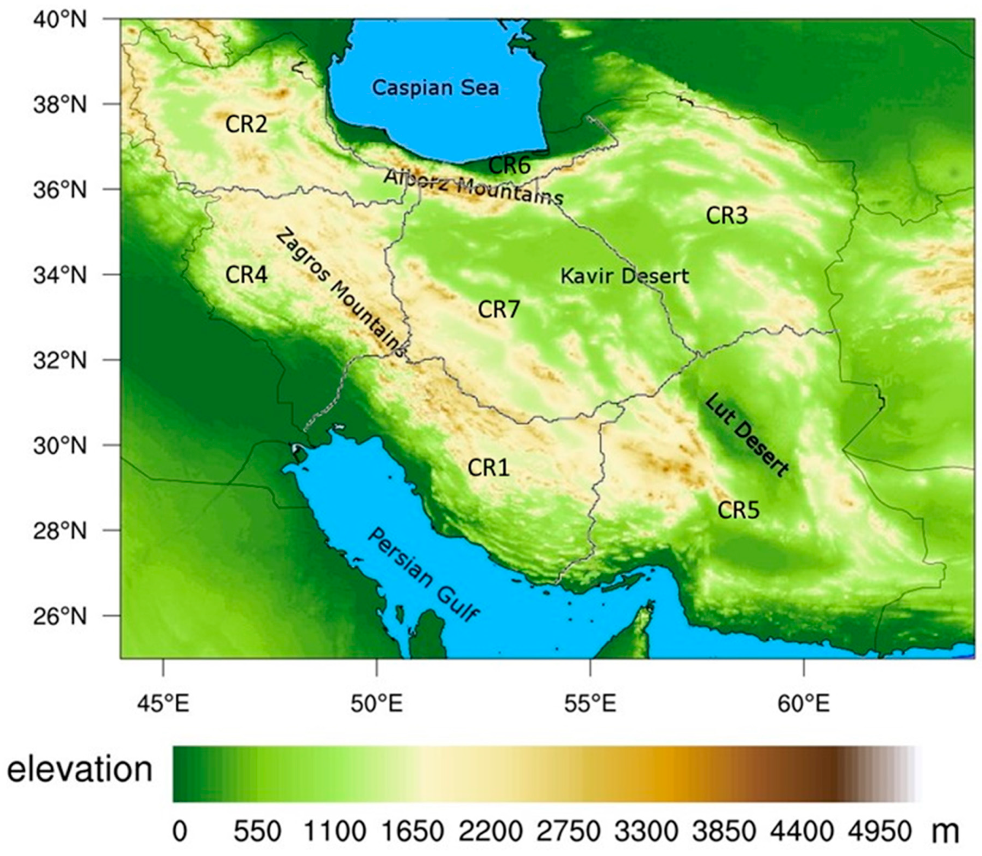
2.1. Study Area

Iran is located in a subtropical region between 25° N and 40° N and between 44° E and 64° E about 1,640,000 km2 (Figure 1). Based on the De Martonne [37] climate classification, the most central parts of the country (that are covered by two great deserts: Lut and Kavir) are categorized as arid and semiarid climates [38]. The country includes a high topography, so that altitudes vary from about 20 m below the mean sea level (on the coast of the Caspian Sea) and more than 5600 m above the mean sea level (in the Alborz Range), both in the Northern part of the country (Figure 1). The Zagros Range in the west and the Alborz Range in the north of the country have an important role in the spatial distribution of precipitation over different parts of Iran. While the mean annual precipitation in Iran is about 250 mm, it varies from less than 50 mm in desert areas to more than 1500 mm on the coast of the Caspian Sea. Most parts of the country have a precipitation regime with a strong seasonality, so that the most annual precipitation occurs in the winter and spring. The rainfall pattern over Iran is affected by the Mediterranean low-pressure system from the west, the Siberian high-pressure system from the north and the Sudan low-pressure from the southwest [39,40]. The synoptic systems, geographical location and complex topography cause a great diversity of climates and rainfall patterns in the region.

2.2. Data

The data employed in this study includes the PERSIANN-CCS rainfall estimates, which is a near-real-time (RT) and quasi-global dataset developed by the Center for Hydrometeorology and Remote Sensing, University of California, Irvine, CA, USA [1,35], as well as historical rain-gauge data. The PERSIANN-CCS algorithm applies an artificial neural network model to the infrared brightness temperature images provided by geostationary satellites and uses passive microwave observations from low-orbit satellites to update its parameters. Cloud patches are extracted from satellite imagery and used to prepare cloud classification groups. The rainfall rate in each pixel is then calculated from the brightness temperature using classified cloud cluster data, histogram matching and exponential regression techniques. The dataset provides hourly precipitation at a resolution of 0.04° × 0.04° over the globe (60° S–60° N), with a latency of about one hour, and it is available from January 2003 to the present.
The rain-gauge network in Iran is mainly operated by the Islamic Republic of Iran’s Meteorological Organization (IRMO) and the Iran Water Resources Management Co (IWRM). The rain-gauge dataset that we used in this study is obtained from these two agencies. Gauges with a large number of missing, unrealistic, erroneous and/or nonphysical values were removed during the preprocessing step. The preprocessing step included an outlier test and double-mass curve analysis. Among all the 1296 rain gauges from IRMO and 104 rain gauges from IWRM, 1130 homogenous gauges with lower density coverage over deserts were selected with a time period from December 2008 to November 2018.
In this study, winter includes December, January and February (DJF); spring includes March, April and May (MAM); summer includes June, July and August (JJA) and autumn includes September, October and November (SON). Therefore, the calibrations and validations started on December and ended at the end of November to include four full seasons for each year, allowing a seasonal analysis of the data for every year. Hence, the calibration period started from the beginning of December 2008 to the end of November 2016, and the validation period started from December 2016 to November 2018. As the accumulation time of gauged daily precipitation was in local time, 3-hourly PERSIANN-CCS data was converted to daily to match the local time.

3. Methods

In order to assess and remove the systematic error of the PERSIANN-CCS daily precipitation, we divided Iran into seven CRs. The accuracy of the QM approach depends on the sample size (number of rainy days in our study) that is used to calculate the CDF. Since Iran is a semi-arid region, the limited number of rainy days in most parts of the country can hinder constructing a reliable CDF for a single or few gauges and pixels. Therefore, to enlarge the sample size, we divided Iran into seven CRs based on the precipitation pattern of the rain gauges. Then, CDFs were generated for the daily rainfalls of each CR and season for both the gauge and PERSIANN-CCS data. Finally, we applied a low-pass filter along with the QM method using the CDFs derived in the previous step to generate the gridded bias-corrected PERSIANN-CCS, called the PERSIANN-CCS-Bias-Corrected. We employed multiple statistical metrics to evaluate the performance of the PERSIANN-CCS and PERSIANN-CCS-Bias-Corrected. Hereafter, the PERSIANN-CCS and PERSIANN-CCS-Bias-Corrected are referred to as the CCS and CCS-BC, respectively.

3.1. Climate Regions

Regionalization of the study area is a common practice in the spatiotemporal analysis of precipitation [39,40,41,42]. Several studies have divided Iran into multiple CRs using different approaches, leading to different CR maps. According to the spatial distribution of the seasonal precipitation regimes point of view, Raziei [43] showed that, from the 24 possible precipitation regimes over the globe, eight were found in Iran. The rainfall regionalization depends on the classification method, as well as the number of stations and spatial distributions of the employed rain gauges. However, despite the differences, some similarities exist in the resulting regionalization maps. For example, all the maps have the same CR by the Caspian Sea, a CR in the northwest of the country and a CR in the west of the country. Nevertheless, there are some differences between the regionalized maps in the center and eastern parts of the country due to the sparse distribution of the rain gauges. In this study, we applied a K-means procedure [44] to our ground data to distinguish seven CRs based on the amounts of precipitation and gauge locations, in addition to the topographic information. Here, we assigned more weight to the distance between the gauges in the K-means process to make sure that the distant gauges with similar precipitation patterns were not grouped together. The final results are shown in Figure 1, which are similar to Raziei [45], who applied the S-mode principal component analysis (PCA) and cluster analysis (CA) procedures, along with the T-mode PCA to 155 synoptic-station data, which resulted in five CRs. Although, using more CRs results in more homogenous precipitation areas, and we used only seven regions to have sufficient data for constructing CDFs for each region.
Figure 1 shows the seven different CRs used in this study. Table 1 shows the areal averages of the annual precipitation for the gauge observations, CCS and CCS-BC for the calibration period in each climate region. CR1 is located in the southwest of Iran along the Persian Gulf. It has a marked seasonality, so most of the annual precipitation falls in the winter and spring, with a very dry summer and moderate autumn [39]. The mid-tropospheric trough over Iraq and the Arabian anticyclone brings moisture from the Persian Gulf, as well as topographic effects that are responsible for the precipitation pattern in this region [39]. CR2 is covered by the high elevation Alborz and Zagros Ranges located in the northwest of the country. This region is mostly influenced by the mid-latitude Westerlies and the Siberian high-pressure system and experiences a high spring (MAM) rainfall. The area features a pronounced seasonality and dry season in the summer [43]. CR3 is located in the northeast of Iran. A trough with its axis over the Caspian Sea and the anticyclonic circulation from the Arabian Sea are responsible for precipitation in this area [39]. The seasonality of this region is very similar to CR1. CR4 is located in the western part of the study area and includes the mountainous areas of the Zagros Range. This region is strongly influenced by Mediterranean low pressures from the west and, sometimes, the atmospheric systems that migrate from the Red Sea [39]. The majority of the annual precipitation occurs in the winter and spring in this area. CR5 is an arid region with a long summer in the southeast of the country. Sometimes, the southern parts of this region experience high-intensity monsoon rainfalls. CR6 is a narrow coastal line along the coast of the Caspian Sea (in the north of the country), and it has the highest annual precipitation (Table 1) in the country, with a moderate seasonality, the highest precipitation in the autumn and the lowest portion of annual precipitation in the summer. The rainfall regime in this area is mostly orographic due to its closeness to the Caspian Sea and the Alborz Range. The summer precipitation is from warm convective clouds that rise over the Alborz Mountains. The pressure gradient due to the Asian high and thermal lows over the Caspian Sea that leads to Easterlies and North-easterlies is considered the reason for high precipitation during the autumn [40]. CR7 is an arid region that includes two large deserts located in the central part of the country. This region that covers a large portion of the country also includes some high elevation areas with rainfalls more abundant than in flat areas.

3.2. Nonparametric Quantile Mapping and Bias Corrections

The popular nonparametric quantile mapping method matches the empirical CDF of the satellite precipitation estimations to that of gauges using a transfer function. The method for calculating the empirical CDFs is explained by Wilks [46] and employed for the QM of daily precipitations from the climate models by Themeßl et al. [32]. In this study, the empirical CDFs are derived for every CR and dataset. Then, a CDF-matching procedure is performed to adjust the satellite-based precipitation data. The matching procedure employed here can be expressed mathematically as:
P CCS BC = CDF G 1 ( CDF CCS ( P CCS ) )
where P CCS BC is the corrected precipitation amount, P CCS is the precipitation amount to be corrected, CDF G 1 is the inverse of the seasonal empirical CDF of the rain-gauge observations and CDF CCS is the seasonal empirical CDF of the CCS. Using this procedure, the daily precipitations of the CCS at each quantile are replaced with the daily precipitations of rain gauges at the same quantile. In other words, the exceedance probability of the precipitation amount of the CCS is calculated using the empirical CDF derived for the CCS for that particular region. Then the empirical CDF of the ground observation are used to find the precipitation associated with the probability. Through this CDF-matching process, the amount of daily precipitation for each pixel of the CCS is adjusted according to the empirical CDF derived for the CCS and gauge observations for each region. This procedure adjusts not only the mean, standard deviation and quantiles of the satellite data but, also, preserves the extreme rainfall amounts [32]. The effects of seasonality is included in the study by generating seasonal CDFs for each region.

3.3. Low-Pass Quantile Mapping Filter

In this step, we apply a filter to generate the final CCS-BC product using a 0.6° × 0.6° filter along with the QM to generate smooth gridded data. Since the resolution of the CCS and CCS-BC are 0.04° × 0.04°, the filter size is selected to be a multiplier of this grid size. The concept of the employed filter is similar to a low-pass filter. However, rather than applying the filter to the values of the bias-corrected CCS, each filter applies the nonparametric QM method based on the convolved region. In other words, a 0.6° × 0.6° is constructed around each selected 0.04° × 0.04° pixel, and the selected 0.04° × 0.04° pixel is bias-corrected according to all the CRs covered by the filter (CDFs from the covering regions) using the nonparametric QM approach. These bias-corrected values are then weight-averaged according to the areas covered by the 0.6° × 0.6° filter and assigned as the bias-corrected value to the selected 0.04° × 0.04° pixel. We explored different filter sizes for this purpose. However, after multiple trials, we realized that using a very small filter led to distinct precipitation patterns for each CR, and using large filters affected the quality of the CCS-BC, especially for narrow regions like the southern part of the Caspian Sea (CR6). Hence, we selected a 0.6° × 0.6° box filter to address these issues and applied this filter to the whole study area.

3.4. Evaluation Metrics

The performances of the CCS and CCS-BC are evaluated using the root mean square error (RMSE), mean bias (BIAS) and correlation coefficient (CORR) between the SPE data and gauge observations as the reference. These metrics are derived as follows:
RMSE = i = 1 n ( S i G i ) 2 n
BIAS = i = 1 n ( S i G i ) n
CORR = c o v ( S , G ) v a r ( S )   v a r ( G )
where S = { S 1 , , S n } and G = { G 1 , , G n } denote the satellite rainfall and gauge rainfall, respectively. The cov() and var() represent the covariance and variance operators, respectively. Obviously, the increased CORR and reduced RMSE and BIAS after bias correction indicates that the CCS-BC outperforms the CCS and reveals the effectiveness of the approach. In addition, some categorical statistics, including the probability of detection (POD), false alarm ratio (FAR) and Heidke skill score (HSS), are derived for the daily evaluations [46].

4. Results

The study area includes a high spatial precipitation variability and high seasonality. Therefore, the calculations are required to be applied to seasonal temporal resolution and, also, CR spatial resolutions (Figure 1).
Therefore, the empirical CDF of the CCS daily precipitation for each 0.04° × 0.04° pixel, as well as the empirical CDF of the daily precipitation of the point scale rain-gauges, are constructed for each season and CR for the calibration. Then, we applied the low-pass QM filter using Equation (1) to bias-correct the CCS daily precipitation in each 0.04° × 0.04° pixel using the derived CDFs for each CR and season. The accuracy of the QM corrections in the spatial pattern and temporal spread are evaluated using statistical indices (Equations (2)–(4)) against the rain-gauge observations during the calibration and validation periods. Figure 2 represents the CDF of the seasonal daily precipitation for the CCS and gauge observations for the seven CRs and four seasons. Table 1 and Figure 2 both demonstrate the systematic bias of the CCS in comparison to the rain-gauge daily precipitation in each region. Table 1 shows the areal average of the mean precipitation for the CRs. These values show the average of the mean areal precipitation for the gauge observations, CCS and CCS-BC for each CR for the calibration period. The CCS generally overestimates the daily precipitation in most CRs and underestimates the daily precipitation in CR1 (winter), CR6 (summer and autumn) and CR4 (winter and autumn). This can also be observed in Figure 2. For instance, considering CR2 in the winter, the 95th percentile of the gauge observation is around 5 mm/day, while the 95th percentile of the CCS is around 15 mm/day. This shows that the CCS is overestimating the precipitation in this region for the winter. We further evaluated the spatial and temporal performances of the CCS and CCS-BC, subsequently.

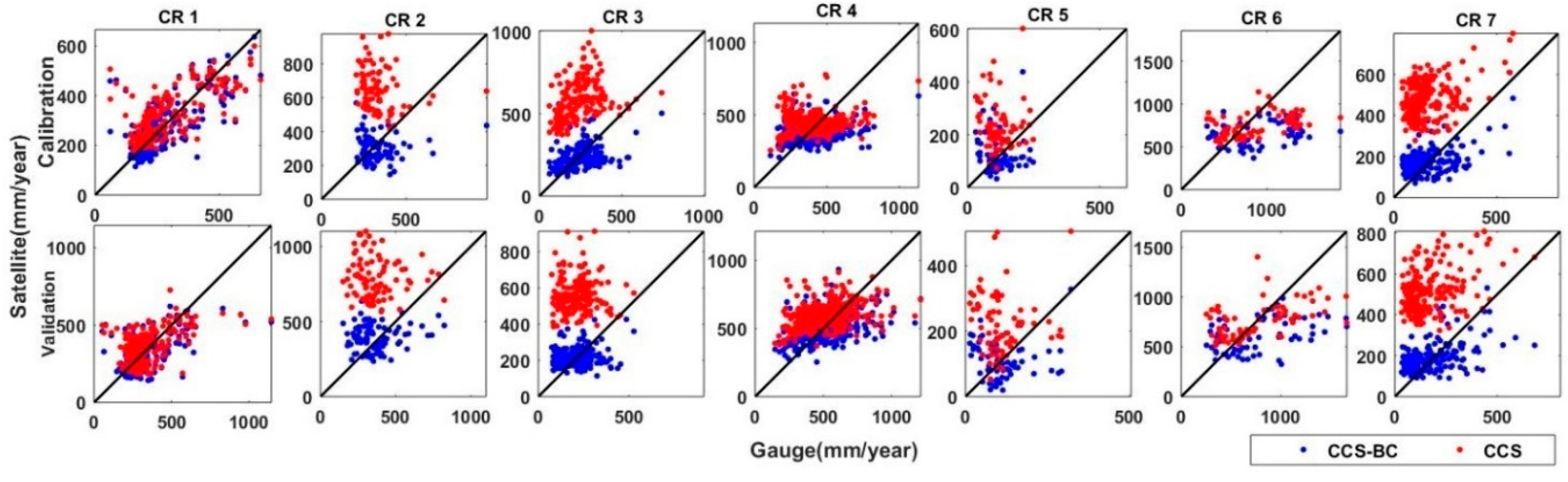
4.1. Spatial Evaluations

The average annual precipitation for the CCS, CCS-BC and gauge for the calibration and validation time periods are shown in Figure 3. These maps show that, in general, the CCS overestimated the annual precipitation in the northern parts of the country. As evident from the figure, the bias correction of the CCS improved the CCS spatial pattern of the mean annual rainfall for both the calibration and validation periods. On the other hand, CCS underestimates the mean annual precipitation over the coast of the Caspian Sea (CR6), especially in the western parts, even after the bias corrections. Many studies have mentioned the poor performance and significant underestimation of different satellite-based precipitation estimations over this region [20,24,25]. The narrow coastal region, which is the wettest part of the country, is located in the Southern part of the Caspian Sea and surrounded by the Alborz Range (more than 5000 m). The rainfall regime in this area is mostly orographic due to its closeness to the Caspian Sea and Alborz Range. Different studies [47,48,49] showed that satellite products have limitations in representing the warm rain processes associated with the convective–orographic cloud formations. Both the satellite and gauge datasets showed a significant difference between the annual precipitation of the Northern and Southern parts of the Alborz Range, since the Alborz Range behaves like a high wall and prevents moisture from passing the mountains. The gauge as the reference dataset showed high annual precipitation over the West of the Zagros Range (CR1 and CR4), especially in high elevation areas, which was captured by the CCS-BC (after bias correction). The overestimations of the CCS in the Central and the Southeastern parts of the country were corrected in the CCS-BC not only for the calibration period but, also, for the validation period, which showed the effectiveness of the applied method. To compare the annual rainfall from the satellite and gauge in each climate region, the scatter plots of the average annual rainfall at the gauged pixels versus the CCS, as well as the CCS-BC, for each CR are shown in Figure 4. The scatter plots illustrate that the QM bias correction approach enhances the annual rainfall amount in most CRs. A quantitative assessment of the spatial pattern of the CCS and CCS-BC annual averaged precipitations for the calibration and validation periods are presented in Table 2 and Table 3, respectively.
Figure 5 and Figure 6 show the spatial patterns of the mean seasonal precipitation for the CCS, CCS-BC and gauge in each CR for the calibration and validation periods, respectively. The gauge interannual distribution of the precipitation with a dry summer and autumn shows a severe seasonality in most parts of the country. However, most annual precipitations fall in the winter and spring in most CRs, but the autumn precipitation includes the highest portion of annual precipitation in CR6. Compared to the gauge, the CCS overestimates the winter and spring rainfall amounts over northern parts of Iran for both the calibration and validation periods. Figure 5, Figure 6, Figure 7 and Figure 8 indicate that the QM successfully reduces the systematic bias for seasonal precipitation not only for the calibration but, also, for the validation time periods (statistics are shown in Table 2 and Table 3). As presented in Table 1 and Table 2, the CCS overestimates the annual precipitation in most CRs, but it underestimates the annual precipitation in CR6. In this region, most of the annual precipitation falls in the autumn, and the CCS underestimates the autumn precipitation. As most of the rainfall over CR6 is from warm orographic clouds that are not effectively detected by satellites, the CCS has a poor performance in this region, and the improvement from the bias-correction approach is not significant. The CCS has a better performance in CR1 in comparison to other CRs (higher CORRs and lower RMSEs and BIASs), and the performance is improved after the bias correction. However, for the annual precipitation, the areal average (excluding CR6) of the RMSEs reduces by 137.5 mm/year (56%), and the areal average (excluding CR6) of the BIASs reduces by 179 mm/year (about 100%), but the CORRs show small increases in some regions (by about 7%) during the calibration period. The bias correction with respect to the annual precipitation improves the RMSEs in all the CRs (excluding CR6) from 5.4 mm/year (1.8% annual precipitation) for CR1 to 249 mm/year (155% mean annual precipitation) for CR7 for the calibration period. The bias correction with respect to winter precipitation improves the RMSEs from 2.8 mm/season (1.8% mean winter precipitation) for CR4 to 103.8 mm/season (182.5% winter precipitation) for CR7 for the calibration period. Similar results for RMSE enhancements for the spring precipitation in CR4 and CR7 indicate that the bias correction in relatively flat areas such as CR7 is more effective than in high topographic regions like CR4. Figure 6 shows the scatter plots of the areal averages of the seasonal precipitations for the CCS and CCS-BC with respect to the gauge data in each CR for the calibration period. The CCS overestimates most seasonal precipitations, which are dominant in CR2, CR3 and CR7, but, after the bias adjustments, the estimations significantly reduce to values close to the gauge seasonal precipitations. In CR6 (the wettest area among the other CRs), the bias-correction approach has slightly improved the performance of the CCS-BC, but it still underestimates the precipitation, especially for autumn, which is the most humid season in this area. This is due to the limitations of the SPEs, which are discussed in the methodology section.
Figure 7 shows the average seasonal precipitation map for the CCS, CCS-BC and gauge data. The maps show that the CCS substantially overestimates the spring precipitation in the northern half of the country during the validation period, which has been functionally corrected by the QM technique. The scatter plots of the areal mean of the seasonal precipitation for the CCS and CCS-BC against the gauge are shown in Figure 8. The quantities of the annual and seasonal statistics for the validation period are shown in Table 3. The areal average (excluding CR6) of the annual RMSEs and BIASs decrease significantly (157 mm/year and 220mm/year, respectively), whereas the areal average of CORRs show a slight change (Table 3 and Figure 3 and Figure 4). Similar to Figure 6 (calibration period), Figure 8 (validation period) shows that the CCS overestimates the winter and spring rainfall amounts (which comprise the majority of the annual rainfall) in CR2, CR3 and CR7. On the other hand, the CCS-BC has improved the winter and spring seasonal precipitation for these CRs compared to the gauge, even for the validation years. According to Table 3, the average (excluding CR6) annual precipitation RMSEs are reduced by 56%, and the average BIASs are decreased by 98% during the validation period. Although the seasonal average RMSEs and BIASs are reduced strongly after the bias correction, there are no significant changes for the CORR. As illustrated in Table 3, the mean seasonal CORRs increased by 111%, 59% and 17%; the RMSEs reduced by 54%, 65% and 66% and the BIASs decreased by 95%, 98% and 95% after the bias correction for CR2, CR3 and CR7, respectively. This means that the spatial disagreements between the satellite estimations and gauge observations decreased in CR2, CR3 and CR7 after the bias adjustment, which agrees with Figure 8.

4.2. Temporal Evaluations

In this section, we evaluate the time series of the areal mean of the monthly precipitation in the gauged pixels for the CCS and CCS-BC for each CR. Figure 9 shows the timeseries of the CCS, CCS-BC and gauge data for the calibration and validation periods. These timeseries are derived by areal averaging the monthly precipitation amounts for each CR and product. According to Figure 9, the CCS overestimates the monthly areal mean precipitations in most regions for both the calibration and validation periods. On the other hand, these systematic biases are removed effectively after the bias corrections in the CCS-BC. The relatively high temporal correlations between the CCS and gauge observations indicate that the temporal variations of the monthly precipitation estimations of the CCS are consistent with the gauge observations, even for the validation period. All statistics improved after the bias corrections. The average CORR, RMSE and BIAS for each calibration period for the CRs (excluding CR6) were 0.717, 31.5 and 16 mm/month and changed to 0.753, 14 and −1 mm/month, respectively. However, the CORRs reduced on average (except CR6) by 4%, and the average of the RMSEs and BIASs decreased by 47% and 96%, respectively, during the validation period.
The results of daily scale evaluations, including the CORR, RMSE and BIAS, as well as the categorical statistics (POD, FAR and HSS) for the calibration and validation periods, are shown in Table 4. A one-mm threshold is employed for deriving the categorical statistics for the timeseries of each region. The statistics are calculated from the timeseries of the areal average of the CCS and CCS-BC daily precipitation estimations in the gauged pixels in each climate region compared to the timeseries of the areal average of the gauge daily observations in the gauged pixels in the same CR. The CCS has a better performance in CR1 in comparison to other CRs (lowest BIAS and highest CORR) and a poor performance in CR6 for the calibration and validation periods. The CORRs of the CCS vary from 0.11 for CR6 to 0.71 for CR1 during the calibration period. There are small changes after the bias corrections. The average RMSE in the CRs (except CR6) reduced by 31% and 26% after the bias corrections for the calibration and validation periods, respectively. Moreover, the average BIAS in the CRs (except CR6) reduced by 106% and 96% after the bias correction for the calibration and validation periods, respectively. However, the mean FAR of the country (excluding CR6) improved slightly after the bias correction (decreases by 7% and 14% for the calibration and validation periods, respectively), but the average POD of the country (excluding CR6) reduced by about 9% and 21%, while the HSS reduced by 7% and 5% for the calibration and validation periods, respectively. The overall bias correction significantly improved the accuracy statistics (RMSE and BIAS) and categorical statistics (FAR and HSS) for the areal average of the daily precipitations.

5. Summary and Conclusions

The objective of this paper was to assess the QM method bias corrections of the PERSIANN-CCS daily precipitation estimations using daily rain gauge observations over Iran. The CCS is a real-time satellite-based dataset that can be used for flood forecasting and hydrological studies. The main findings of this study can be summarized as follows:
  • The QM bias correction approach is an effective method for the bias correction of satellite-based precipitation products upon availability of the ground-based precipitation observations.
  • The QM method can be trained on historical data to effectively bias-correct future remotely sensed observations.
  • The CCS have poor performances in representing the precipitation rates and patterns in the Northern part of Iran (CR6), and QM is not effective in bias-correcting the CCS in this region due to its orographic and climatic conditions.
The seasonal CDFs of the daily gauge observations, as well as the CCS daily precipitation estimations, are employed to remove the systematic bias from the CCS estimates in seven different climate regions. The CCS has a better performance in CR1 in comparison to other CRs, which means it can better detect clouds in this area than in other regions. The results of some regional studies indicate that the Southern water bodies such as the Persian Gulf, the Oman Sea and the North Indian Ocean are the main sources of cloud moisture in this region [50,51]. The results show that the spatial distribution of the satellite estimates effectively improves after the bias corrections for the mean annual and mean seasonal precipitations in most CRs (except CR6) not only for the calibration period but, also, for the validation period. The areal average of the annual RMSEs and BIASs reduced by 137.5 mm/year (56%) and 179 mm/year (100%), respectively, during the calibration period (2009–2016). Additionally, the average (excluding CR6) of the annual precipitation RMSEs reduced by 157 mm/year (56%), and the average BIAS decreased by 220 mm/year (98%) during the validation period. As the CCS overestimates the annual and seasonal (winter and spring) precipitations in the Northern half of the country, the improvement of the bias corrections is significant in CR2, CR3 and CR7. The CCS underestimated the annual precipitation in CR6 and had a poor performance after the bias corrections. Previous studies [20,24,25] have shown that different satellite products have poor performances over this area. In fact, most rainfall results from warm orographic clouds that rise above the Alborz Mountains are not captured by satellites.
The results for the validation period indicate that the historical rain gauge data and the QM bias correction method can be effective in reducing the systematic bias of the satellite precipitation estimations in the future. Obviously, more historical data that covers year-to-year precipitation variations would help to make more accurate CDFs and lead to further improvements for satellite estimates after bias corrections. In this bias correction method, we do not need concurrent rain gauge data, which are important for real-time SEPs. However, for constructing CDFs in each CCS pixel (0.04°), or even a 1° × 1° box (as used by Yang et al. [34]), sufficient samples are necessary, but rain gauges are sparse in mountainous and desert areas such as Iran. Therefore, using climate regions with homogenous precipitation patterns as employed in this study and other similar works [36] would be an appropriate method to overcome this restriction in similar areas. Furthermore, using climate regions revealed the distinguished effects of bias corrections in different climates. Overall, the QM method reduced the bias in the annual, seasonal and monthly scales, but random errors caused by day-to-day precipitation variations remained as expected.

Author Contributions

Conceptualization, P.-S.K.-B., M.R.N. and A.A.A.; methodology, P.-S.K.-B., M.R.N., A.A.A. and K.-l.H.; software, M.R.N.; resources, S.S.; data curation, A.C., P.-S.K.-B. and M.R.N.; supervision, S.S., K.-l.H. and P.-S.K.-B.; funding acquisition, S.S., K.-l.H., A.C. and P.-S.K.-B.; writing-original draft preparation, P.-S.K.-B.; writing-review and editing, P.-S.K.-B., M.R.N., A.A.A., A.C., K.-l.H. and S.S. All authors have read and agreed to the published version of the manuscript.

Funding

This work was partially funded by UNESCO G-WADI program (Contract 4500330747), UC Lab Research Program (Grant ID No. 116849) and a visiting scholar grant from the Islamic Azad University Tehran North Branch.

Acknowledgments

The authors acknowledge and thank the Islamic Republic of Iran’s Meteorological Organization (IRIMO) and the Iran Water Resources Management Co for providing the rain gauge data. This work was supported by a grant to the first author (P.S.K.B.) from the Islamic Azad University Tehran North Branch, while she stayed at CHRS, University of California, Irvine, CA, USA as a visiting researcher. The co-authors affiliated with CHRS acknowledge the partial support for the preparation of data and research support received for the UNESCO G-WADI program and the support received from the University of California, Irvine Henry Samueli School of Engineering.

Conflicts of Interest

The authors declare no conflicts of interest.

References

  1. Hsu, K.; Gao, X.; Sorooshian, S.; Gupta, H.V. Precipitation estimation from remotely sensed information using artificial neural networks. J. Appl. Meteorol. 1997, 36, 1176–1190. [Google Scholar] [CrossRef]
  2. Huffman, G.J.; Adler, R.F.; Stocker, E.; Bolvin, D.T.; Nelkin, E.J. Analysis of TRMM 3-hourly multi-satellite precipitation estimates computed in both real and post-real time. In Proceedings of the 12th Conference on Satellite Meteorology and Oceanography, Long Beach, CA, USA, 9–13 February 2003. [Google Scholar]
  3. Joyce, R.J.; Janowiak, J.E.; Arkin, P.A.; Xie, P. CMORPH: A method that produces global precipitation estimates from passive microwave and infrared data at high spatial and temporal resolution. J. Hydrometeorol. 2004, 5, 487–503. [Google Scholar] [CrossRef]
  4. Beck, H.E.; Van Dijk, A.I.J.M.; Levizzani, V.; Schellekens, J.; Gonzalez Miralles, D.; Martens, B.; De Roo, A. MSWEP: 3-hourly 0.25 global gridded precipitation (1979–2015) by merging gauge, satellite, and reanalysis data. Hydrol. Earth Syst. Sci. 2017, 21, 589–615. [Google Scholar] [CrossRef] [Green Version]
  5. Funk, C.C.; Peterson, P.J.; Landsfeld, M.F.; Pedreros, D.H.; Verdin, J.P.; Rowland, J.D.; Romero, B.E.; Husak, G.J.; Michaelsen, J.C.; Verdin, A.P. A quasi-global precipitation time series for drought monitoring. USA Geol. Surv. Data Ser. 2014, 832, 1–12. [Google Scholar]
  6. Chen, K.; Guo, S.; Wang, J.; Qin, P.; He, S.; Sun, S.; Naeini, M.R. Evaluation of GloFAS-Seasonal Forecasts for Cascade Reservoir Impoundment Operation in the Upper Yangtze River. Water 2019, 11, 2539. [Google Scholar] [CrossRef] [Green Version]
  7. AghaKouchak, A.; Mehran, A.; Norouzi, H.; Behrangi, A. Systematic and random error components in satellite precipitation data sets. Geophys. Res. Lett. 2012, 39. [Google Scholar] [CrossRef] [Green Version]
  8. Kimani, M.W.; Hoedjes, J.C.B.; Su, Z. An assessment of satellite-derived rainfall products relative to ground observations over East Africa. Remote Sens. 2017, 9, 430. [Google Scholar] [CrossRef] [Green Version]
  9. Tang, L.; Tian, Y.; Yan, F.; Habib, E. An improved procedure for the validation of satellite-based precipitation estimates. Atmos. Res. 2015, 163, 61–73. [Google Scholar] [CrossRef]
  10. Sadeghi, M.; Asanjan, A.A.; Faridzad, M.; Nguyen, P.; Hsu, K.; Sorooshian, S.; Braithwaite, D. PERSIANN-CNN: Precipitation Estimation from Remotely Sensed Information Using Artificial Neural Networks–Convolutional Neural Networks. J. Hydrometeorol. 2019, 20, 2273–2289. [Google Scholar] [CrossRef]
  11. Serrat-Capdevila, A.; Merino, M.; Valdes, J.B.; Durcik, M. Evaluation of the performance of three satellite precipitation products over Africa. Remote Sens. 2016, 8, 836. [Google Scholar] [CrossRef] [Green Version]
  12. Sun, Q.; Miao, C.; Duan, Q.; Ashouri, H.; Sorooshian, S.; Hsu, K. A review of global precipitation data sets: Data sources, estimation, and intercomparisons. Rev. Geophys. 2018, 56, 79–107. [Google Scholar] [CrossRef] [Green Version]
  13. Zhu, Q.; Xuan, W.; Liu, L.; Xu, Y.P. Evaluation and hydrological application of precipitation estimates derived from PERSIANN-CDR, TRMM 3B42V7, and NCEP-CFSR over humid regions in China. Hydrol. Process. 2016, 30. [Google Scholar] [CrossRef]
  14. Kimani, M.W.; Hoedjes, J.C.B.; Su, Z. Bayesian Bias Correction of Satellite Rainfall Estimates for Climate Studies. Remote Sens. 2018, 10, 1074. [Google Scholar] [CrossRef] [Green Version]
  15. Tan, M.L.; Ibrahim, A.L.; Duan, Z.; Cracknell, A.P.; Chaplot, V. Evaluation of six high-resolution satellite and ground-based precipitation products over Malaysia. Remote Sens. 2015, 7, 1504–1528. [Google Scholar] [CrossRef] [Green Version]
  16. Sohn, B.J.; Han, H.-J.; Seo, E.-K. Validation of satellite-based high-resolution rainfall products over the Korean Peninsula using data from a dense rain gauge network. J. Appl. Meteorol. Climatol. 2010, 49, 701–714. [Google Scholar] [CrossRef]
  17. Tapiador, F.J.; Turk, F.J.; Petersen, W.; Hou, A.Y.; García-Ortega, E.; Machado, L.A.T.; Angelis, C.F.; Salio, P.; Kidd, C.; Huffman, G.J. Global precipitation measurement: Methods, datasets and applications. Atmos. Res. 2012, 104, 70–97. [Google Scholar] [CrossRef]
  18. Nguyen, P.; Ombadi, M.; Sorooshian, S.; Hsu, K.; AghaKouchak, A.; Braithwaite, D.; Ashouri, H.; Thorstensen, A.R. The PERSIANN family of global satellite precipitation data: A review and evaluation of products. Hydrol. Earth Syst. Sci. 2018, 22, 5801–5816. [Google Scholar] [CrossRef] [Green Version]
  19. Dinku, T.; Ceccato, P.; Cressman, K.; Connor, S.J. Evaluating detection skills of satellite rainfall estimates over desert locust recession regions. J. Appl. Meteorol. Climatol. 2010, 49, 1322–1332. [Google Scholar] [CrossRef]
  20. Moazami, S.; Golian, S.; Kavianpour, M.R.; Hong, Y. Comparison of PERSIANN and V7 TRMM Multi-satellite Precipitation Analysis (TMPA) products with rain gauge data over Iran. Int. J. Remote Sens. 2013, 34, 8156–8171. [Google Scholar] [CrossRef]
  21. Thiemig, V.; Rojas, R.; Zambrano-Bigiarini, M.; Levizzani, V.; De Roo, A. Validation of satellite-based precipitation products over sparsely gauged African river basins. J. Hydrometeorol. 2012, 13, 1760–1783. [Google Scholar] [CrossRef]
  22. Guo, H.; Chen, S.; Bao, A.; Hu, J.; Gebregiorgis, A.S.; Xue, X.; Zhang, X. Inter-comparison of high-resolution satellite precipitation products over Central Asia. Remote Sens. 2015, 7, 7181–7211. [Google Scholar] [CrossRef] [Green Version]
  23. Dinku, T.; Ruiz, F.; Connor, S.J.; Ceccato, P. Validation and intercomparison of satellite rainfall estimates over Colombia. J. Appl. Meteorol. Climatol. 2010, 49, 1004–1014. [Google Scholar] [CrossRef]
  24. Javanmard, S.; Yatagai, A.; Nodzu, M.I.; BodaghJamali, J.; Kawamoto, H. Comparing high-resolution gridded precipitation data with satellite rainfall estimates of TRMM 3B42 over Iran. Adv. Geosci. 2010, 25. [Google Scholar] [CrossRef] [Green Version]
  25. Katiraie-Boroujerdy, P.-S.; Nasrollahi, N.; Hsu, K.-L.; Sorooshian, S. Evaluation of satellite-based precipitation estimation over Iran. J. Arid Environ. 2013, 97. [Google Scholar] [CrossRef] [Green Version]
  26. Katiraie-Boroujerdy, P.-S.; Akbari Asanjan, A.; Hsu, K.-L.; Sorooshian, S. Intercomparison of PERSIANN-CDR and TRMM-3B42V7 precipitation estimates at monthly and daily time scales. Atmos. Res. 2017, 193. [Google Scholar] [CrossRef] [Green Version]
  27. Fang, G.; Yang, J.; Chen, Y.N.; Zammit, C. Comparing bias correction methods in downscaling meteorological variables for a hydrologic impact study in an arid area in China. Hydrol. Earth Syst. Sci. 2015, 19, 2547–2559. [Google Scholar] [CrossRef] [Green Version]
  28. Huffman, G.J.; Bolvin, D.T.; Nelkin, E.J.; Wolff, D.B.; Adler, R.F.; Gu, G.; Hong, Y.; Bowman, K.P.; Stocker, E.F. The TRMM multisatellite precipitation analysis (TMPA): Quasi-global, multiyear, combined-sensor precipitation estimates at fine scales. J. Hydrometeorol. 2007, 8, 38–55. [Google Scholar] [CrossRef]
  29. Xie, P.; Xiong, A. A conceptual model for constructing high-resolution gauge-satellite merged precipitation analyses. J. Geophys. Res. Atmos. 2011, 116. [Google Scholar] [CrossRef]
  30. Katiraie-Boroujerdy, P.; Akbari Asanjan, A.; Chavoshian, A.; Hsu, K.; Sorooshian, S. Assessment of seven CMIP5 model precipitation extremes over Iran based on a satellite-based climate data set. Int. J. Climatol. 2019, 39, 3505–3522. [Google Scholar] [CrossRef]
  31. Piani, C.; Haerter, J.O.; Coppola, E. Statistical bias correction for daily precipitation in regional climate models over Europe. Theor. Appl. Climatol. 2010, 99, 187–192. [Google Scholar] [CrossRef] [Green Version]
  32. Themeßl, M.J.; Gobiet, A.; Heinrich, G. Empirical-statistical downscaling and error correction of regional climate models and its impact on the climate change signal. Clim. Chang. 2012, 112, 449–468. [Google Scholar] [CrossRef]
  33. Osorio, J.D.G.; Galiano, S.G.G. Assessing uncertainties in the building of ensemble RCMs over Spain based on dry spell lengths probability density functions. Clim. Dyn. 2013, 40, 1271–1290. [Google Scholar] [CrossRef]
  34. Yang, Z.; Hsu, K.; Sorooshian, S.; Xu, X.; Braithwaite, D.; Verbist, K.M.J. Bias adjustment of satellite-based precipitation estimation using gauge observations: A case study in Chile. J. Geophys. Res. Atmos. 2016, 121, 3790–3806. [Google Scholar] [CrossRef] [Green Version]
  35. Hong, Y.; Hsu, K.-L.; Sorooshian, S.; Gao, X. Precipitation estimation from remotely sensed imagery using an artificial neural network cloud classification system. J. Appl. Meteorol. 2004, 43, 1834–1853. [Google Scholar] [CrossRef] [Green Version]
  36. Alharbi, R.; Hsu, K.; Sorooshian, S. Bias adjustment of satellite-based precipitation estimation using artificial neural networks-cloud classification system over Saudi Arabia. Arab. J. Geosci. 2018, 11, 508. [Google Scholar] [CrossRef] [Green Version]
  37. De Martonne, E. Treite de Geographie Physique, 7th ed.; Colin, Librairie Armand: Paris, France, 1948. [Google Scholar]
  38. Khalili, A.; Hajjam, S.; Irannejad, P. The General Model of Water and the Climate of Iran, The Fourth Part of Weather Division; Jamab: Tehran, Iran, 1991. [Google Scholar]
  39. Raziei, T.; Mofidi, A.; Santos, J.A.; Bordi, I. Spatial patterns and regimes of daily precipitation in Iran in relation to large-scale atmospheric circulation. Int. J. Climatol. 2012, 32, 1226–1237. [Google Scholar] [CrossRef] [Green Version]
  40. Domroes, M.; Kaviani, M.; Schaefer, D. An analysis of regional and intra-annual precipitation variability over Iran using multivariate statistical methods. Theor. Appl. Climatol. 1998, 61, 151–159. [Google Scholar] [CrossRef]
  41. Modarres, R. Regional precipitation climates of Iran. J. Hydrol. (N. Z.) 2006, 13–27. [Google Scholar]
  42. Roushangar, K.; Alizadeh, F. A multiscale spatio-temporal framework to regionalize annual precipitation using k-means and self-organizing map technique. J. Mt. Sci. 2018, 15, 1481–1497. [Google Scholar] [CrossRef]
  43. Raziei, T. An analysis of daily and monthly precipitation seasonality and regimes in Iran and the associated changes in 1951–2014. Theor. Appl. Climatol. 2018, 134, 913–934. [Google Scholar] [CrossRef]
  44. Arthur, D.; Vassilvitskii, S. K-Means++: The Advantages of Careful Seeding. In Proceedings of the Eighteenth Annual ACM-SIAM Symposium on Discrete Algorithms, SODA ’07, New Orleans, LA, USA, 7–9 January 2007; pp. 1027–1035. [Google Scholar]
  45. Raziei, T. A precipitation regionalization and regime for Iran based on multivariate analysis. Theor. Appl. Climatol. 2018, 131, 1429–1448. [Google Scholar] [CrossRef]
  46. Wilks, D.S. Statistical Methods in the Atmospheric Sciences; Academic Press: Cambridge, MA, USA, 2011; Volume 100, ISBN 0123850223. [Google Scholar]
  47. Hong, Y.; Gochis, D.; Cheng, J.; Hsu, K.; Sorooshian, S. Evaluation of PERSIANN-CCS rainfall measurement using the NAME event rain gauge network. J. Hydrometeorol. 2007, 8, 469–482. [Google Scholar] [CrossRef] [Green Version]
  48. Sorooshian, S.; AghaKouchak, A.; Arkin, P.; Eylander, J.; Foufoula-Georgiou, E.; Harmon, R.; Hendrickx, J.M.H.; Imam, B.; Kuligowski, R.; Skahill, B. Advanced concepts on remote sensing of precipitation at multiple scales. Bull. Am. Meteorol. Soc. 2011, 92, 1353–1357. [Google Scholar] [CrossRef]
  49. Mehran, A.; AghaKouchak, A. Capabilities of satellite precipitation datasets to estimate heavy precipitation rates at different temporal accumulations. Hydrol. Process. 2014, 28, 2262–2270. [Google Scholar] [CrossRef]
  50. Evans, J.P.; Smith, R.B. Water vapor transport and the production of precipitation in the eastern Fertile Crescent. J. Hydrometeorol. 2006, 7, 1295–1307. [Google Scholar] [CrossRef] [Green Version]
  51. Chakraborty, A.; Behera, S.K.; Mujumdar, M.; Ohba, R.; Yamagata, T. Diagnosis of tropospheric moisture over Saudi Arabia and influences of IOD and ENSO. Mon. Weather Rev. 2006, 134, 598–617. [Google Scholar] [CrossRef]
Figure 1. The topography map of Iran and the seven climate regions.
Remotesensing 12 02102 g001
Figure 2. The seasonal cumulative distribution function (CDF) of the daily precipitation for the gauge and Precipitation Estimation from Remotely Sensed Information using Artificial Neural Networks-Cloud Classification System (PERSIANN-CCS) (CCS) estimations for the seven climate regions (CRs) for the calibration period.
Remotesensing 12 02102 g002
Figure 3. Mean annual precipitation for the CCS, PERSIANN-CCS-Bias-Corrected (CCS-BC) and gauge for the calibration and validation periods.
Remotesensing 12 02102 g003
Figure 4. Scatter plots of the CCS and CCS-BC mean annual precipitation versus the gauge mean annual precipitation in gauged pixels for each CR for the calibration and validation periods.
Remotesensing 12 02102 g004
Figure 5. Mean seasonal precipitations of the gauge observation and the CCS and the CCS-BC for the calibration period.
Remotesensing 12 02102 g005
Figure 6. Scatter plots of the CCS and CCS-BC mean seasonal precipitations versus the gauge mean seasonal precipitation in gauged pixels for seven CRs for the calibration period.
Remotesensing 12 02102 g006
Figure 7. Mean seasonal precipitation from the gauge observations and the CCS and the CCS-BC for the validation period.
Remotesensing 12 02102 g007
Figure 8. Scatter plots of the CCS and CCS-BC mean seasonal precipitations versus the gauge mean seasonal precipitation in gauged pixels for the seven CRs for the validation period.
Remotesensing 12 02102 g008
Figure 9. The areal average of the monthly precipitation timeseries in the gauged pixels in each CR for the calibration and validation periods.
Remotesensing 12 02102 g009
Table 1. The areal averages of the mean annual precipitations for the seven climate regions (CRs) for the calibration period. CCS: Precipitation Estimation from Remotely Sensed Information using Artificial Neural Networks-Cloud Classification System (PERSIANN-CCS) and CCS-BC: PERSIANN-CCS-Bias-Corrected.
Gauge (mm/year)CCS (mm/year)CCS-BC (mm/year)
CR1294.1318.6284.5
CR2333.2643.7297.8
CR3246.4593.5239.1
CR4407.7442.0366.6
CR5118.1237.1121.7
CR6882.2752.6653.7
CR7160.3476.7173.3
Table 2. Quantitative results of the spatial evaluations for the mean annual and mean seasonal precipitations of the CCS and CCS-BC compared to the gauge observations for the seven CRs for the calibration period. BIAS: mean bias, CORR: correlation coefficient and RMSE: root mean square error.
AnnualWinterSpringSummerAutumn
CCSCCS-BCCCSCCS-BCCCSCCS-BCCCSCCS-BCCCSCCS-BC
CR1CORR0.70380.73880.63890.68550.62420.58840.69200.64770.8110.8236
RMSE7.16.74.153.654.492.551.390.271.671.54
BIAS24.5−9.59−26.8−3.849.9−3.813−0.1−11.6−1.8
CR2CORR−0.1930.0118−0.323−0.001−0.198−0.1350.64650.6652−0.1600.0793
RMSE38.514.617.45.517.25.422.44.94.6
BIAS310.5−35.4143.38.2143.8−21.95.4−13.518.1−8.1
CR3CORR0.31150.34700.06050.08520.40560.29470.48880.49950.44140.4783
RMSE28.78.310.63.314.53.31.41.23.22
BIAS347.1−7.3123.52.1181.4−11.19.9−0.532.32.2
CR4CORR0.06000.1816−0.097−0.0590.17600.22950.56490.54690.30850.3770
RMSE8.88.24.34.14.12.90.40.22.32.1
BIAS34.4−41.12.1−10.249.7−175.40.04−22.8−13.9
CR5CORR−0.090−0.062−0.107−0.0810.08070.08370.62810.60370.16870.1893
RMSE19.210.48.1693.33.80.921.6
BIAS1193.731.31.860.7220.3−1.36.71.2
CR6CORR0.40.24300.10820.24620.47330.4211−0.147−0.2950.40430.2528
RMSE43.751.61411.821.16.812.711.239.128.6
BIAS−129.5−228.436.6−31.9164.7−24.8−86−59.6−244.8−112.1
CR7CORR0.37080.53670.18430.38170.18950.29360.69390.75630.45850.6250
RMSE23.25.98.22.5122.20.90.72.91.5
BIAS316.413110.16.3165.43.37.50.433.53
Table 3. Quantitative results of the spatial evaluations for the mean annual and mean seasonal precipitation of the CCS and CCS-BC compared to the gauge observations for the seven CRs for the validation period.
AnnualWinterSpringSummerAutumn
CCSCCS-BCCCSCCS-BCCCSCCS-BCCCSCCS-BCCCSCCS-BC
CR1CORR0.4870.5250.0290.1160.5840.0.576−0.023−0.0310.6150.703
RMSE139.2136.585.478.564.946.127.225.853.550.7
BIAS10.8−19.7−42.2−16.744.6−17.1−2−5.110.319.2
CR2CORR−0.0710.141−0.0460.1950.0390.1620.4450.380−0.0040.181
RMSE465151.7126.175.7267.273.52627.996.359.5
BIAS420.921.891.6−38.2254.642.7−0.6−12.575.329.8
CR3CORR−0.0160.082−0.094−0.0380.1800.1760.2480.2630.0090.147
RMSE367.110198.644.5224.147.713.614.365.233.6
BIAS343.55.782.9−15.4216.123.80.8−5.743.72.9
CR4CORR0.3610.4210.2790.3260.2700.2090.1240.1010.2120.353
RMSE183.616492.495.8133.388.326.727.565.564.6
BIAS73.2−5.2−38.8−48.4108.731.4−4.7−8.17.920
CR5CORR−0.043−0.025−0.310−0.2390.3280.2700.2780.2010.4610.381
RMSE166.696.590.269.367.125.929.814.117.415.3
BIAS117.71147.312.752.5−3.310.70.57.21
CR6CORR0.5210.3950.3350.4510.1960.2500.177−0.0850.5050.203
RMSE313.7367.796.4105.1282.888.3156.1155.7257.7225.7
BIAS4.9−145.51.9−60.9272.265.9−89.7−81.6−179.5−68.9
CR7CORR0.3920.4850.1760.2530.2320.2280.5740.4200.2700.564
RMSE36999.9103.246.1222.249.110.812.665.427.3
BIAS384.918.587.4−4.3211.214.1−0.8−3.951.112.5
Table 4. The quantitative and categorical statistic results of the daily evaluations of the areal mean for the CCS and CCS-BC compared to the gauge observations for the seven CRs for the calibration (2009–2016) and validation (2017–2018) periods.
CalibrationValidation
CR1CR2CR3CR4CR5CR6CR7CR1CR2CR3CR4CR5CR6CR7
RMSE (mm/day)CCS2.113.642.792.251.446.902.212.773.283.902.811.336.392.60
CCS-BC1.951.791.652.181.155.521.112.572.172.112.681.135.081.28
BIAS (mm/day)CCS0.060.830.920.140.33−0.370.860.031.110.960.240.330.030.95
CCS-BC−0.02−0.11−0.04−0.080.01−0.630.05−0.050.040.030.010.03−0.370.06
CORRCCS0.710.390.470.670.570.110.530.690.500.270.650.630.110.46
CCS-BC0.760.520.390.690.570.250.500.740.460.240.680.620.280.36
FARCCS0.480.500.570.480.670.500.690.550.490.610.450.750.530.65
CCS-BC0.430.410.480.400.550.490.570.470.410.520.440.590.490.57
PODCCS0.850.830.790.790.820.500.880.750.850.910.750.700.520.86
CCS-BC0.800.610.550.730.600.430.620.700.690.590.650.600.480.54
HSSCCS0.590.500.430.530.430.200.400.480.500.470.500.320.210.43
CCS-BC0.620.470.420.570.470.200.440.530.500.440.460.440.240.40

