Abstract
The Advanced Microwave Sounding Unit (AMSU)-A/Advanced Technology Microwave Sounder (ATMS) onboard the National Oceanic Atmospheric Administration (NOAA)-18/-19, MetOp-A/-B, and Suomi National Polar-orbiting Partnership satellites provide global observations of the cloud Liquid Water Path (LWP) almost 10 times a day. This study explores the possibility of capturing the diurnal cycle of the LWP. An inter-satellite cross-calibration is first carried out using a double-difference method. A remapping is then used to obtain the AMSU-A-like LWP to account for beam shape discrepancies between the ATMS and AMSU-A. We finally examine the diurnal cycle of the LWP over the Southeast Pacific Ocean using the ATMS and AMSU-A data from the five satellites mentioned above. Results show that the remapped ATMS results agree well with the AMSU-A results at the same local time over a stratocumulus region. LWP retrievals from multiple satellite cross-track microwave radiometers can well reproduce the diurnal variation characteristics of LWP in 2015 over the East Pacific Ocean, including the seasonal variation of the diurnal variation. This study presents the first step toward merging LWP data from all ATMS and AMSU-A radiometers and will be of interest to many researchers studying LWP-related weather and climate changes, especially considering the possible loss of higher-resolution microwave-frequency conical-scanning sensors in the coming years.
1. Introduction
Changes in cloud parameters, such as the Liquid Water Path (LWP), on regional, and perhaps even global scales, are associated with cloud feedback mechanisms in the climate system. The monthly mean diurnal variations in LWP were examined in the past using mainly data from satellite conical-scanning microwave imagers. Wood et al. [1] investigated the diurnal cycle of LWP over the subtropical and tropical oceans using the Tropical Rainfall Measuring Mission (TRMM) Microwave Imager (TMI) satellite microwave radiometer data from 1999 and 2000. They pointed out a larger diurnal cycle in the Southeast Atlantic and Pacific subtropical low-cloud regions relative to those in the Northern Hemisphere’s Pacific and Atlantic Oceans. O’Dell et al. [2] and Elsaesser et al. [3] derived an 18-year (1988–2005) and 29-year (1988–2016) climatology of monthly mean LWP, respectively, as well as mean monthly diurnal cycles in 1° × 1° grid boxes based on satellite passive conical-scanning microwave imager observations over the global oceans. A modern retrieval methodology was applied consistently to observations from the Special Sensor Microwave Imager (SSM/I), the TMI, and the Advanced Microwave Scanning Radiometer (AMSR) for Earth Observing System (EOS) microwave sensors on eight different satellite platforms. O’Neill et al. [4] quantified the seasonal and interannual variabilities of the LWP and LWP diurnal and semi-diurnal cycles over the Southeast Pacific Ocean at 30-day intervals using LWP observations made by the AMSR on EOS-Aqua, TMI, and the SSM/I F13 and F15 satellites for the seven-year period of June 2002 to May 2009. The LWP field showed a considerable spatial and seasonal variability throughout the Southeast Pacific, with two distinct annual cycles, one during the austral summer and the other during the austral autumn.
Although many previous efforts have been made to retrieve diurnal LWP data over the global oceans from multiple conical-scanning microwave imager observations, the diurnal characteristics of LWP data from multiple cross-track microwave radiometers have received little attention to date. This study makes use of LWP data from satellite cross-track microwave radiometers to examine the monthly mean diurnal variations in LWP. Polar-orbiting Operational Environmental Satellites (POES) cross-track microwave radiometers have provided more than 20 years of global oceanic cloud LWP data since the launch of the National Oceanic Atmospheric Administration (NOAA)-15 in 1998 carrying the Advanced Microwave Sounding Unit (AMSU)-A. AMSU-A instruments were onboard the subsequent POES satellites NOAA-16, -17, -18, and -19 and MetOp-A, -B, and -C. A more advanced cross-track microwave radiometer called the Advanced Technology Microwave Sounder (ATMS) was first deployed on the Suomi National Polar-orbiting Partnership (S-NPP) satellite and then on the NOAA-20 satellite for the second time. The S-NPP satellite was successfully launched into a circular, near-polar, afternoon-configured (1:30 p.m.± 10 minutes) orbit on 28 October 2011, as the pathfinder for the Joint Polar Satellite System (JPSS) operational satellite series in the United States. The NOAA-20 satellite carrying the ATMS was successfully launched into a sun-synchronous orbit similar to the S-NPP on 18 November 2017. The cloud LWP over oceans can be retrieved from two window channel (microwave frequencies 23.8 and 31.4 GHz) brightness temperature (BT) measurements from both the AMSU-A and ATMS. However, the beam width of these two low-frequency window channels from the ATMS is 5.2°, which is greater than the 3.3° beam width of the AMSU-A channels. To merge the ATMS- and AMSU-A-derived LWP data, the 5.2° beam width must be converted to the 3.3° beam width through a remapping procedure. Fortunately, each ATMS Field of View (FOV) overlaps with its four neighboring FOVs, making it possible for such a remapping to partially overcome the beam-filling effect of subpixel cloud inhomogeneity within coarse ATMS pixels.
The ATMS, built to replace its predecessors, the AMSU-A and the Microwave Humidity Sounder (MHS), has 22 channels at frequencies ranging from 23 to 183 GHz. With the ATMS onboard the next-generation JPSS operational satellite series in the United States, and the AMSU-A and MHS onboard MetOp-A, -B, and -C from the European Organization for the Exploitation of Meteorological Satellites (EUMETSAT), the time series of global microwave measurements can be further extended to well beyond 2028. This offers an opportunity to study climate using a long time series of AMSU-A/ATMS observations. The LWP is a meteorological variable that plays an important role in understanding weather and climate. Knowledge of the LWP is beneficial for developing a cloud detection algorithm required by AMSU-A, MHS, and ATMS data assimilation [5,6]. It also allows one to estimate how much of the AMSU-A/ATMS signal arises from non-oxygen emissions and to evaluate the impacts of both cloud and precipitation on tropospheric and lower stratospheric temperature trends derivable from the AMSU-A/ATMS temperature-sounding channels. Spencer et al. [7] noticed the influence of contamination from precipitation-sized ice in deep convection and cloud liquid water. They concluded that the effects from precipitation-sized ice in deep convection are the largest because ice scattering could cause a BT depression of up to several degrees Celsius. Weng and Zou [8] showed that the global mean temperature in the lower and middle troposphere derived from NOAA-15 AMSU-A data has a larger warming rate (about 20–30% higher) when the cloud-affected BTs are removed from the trend calculation. Including cloud-affected radiances in the trend analysis was also shown to significantly offset the stratospheric cooling represented by AMSU-A channel 9 over the middle and high latitudes of the Northern Hemisphere. The present study will contribute to the establishment of long-term climate data records of LWP over global oceans based on POES cross-track microwave radiometers AMSU-A and ATMS.
The paper is arranged as follows. Section 2 describes some characteristic differences between the AMSU-A and ATMS data, and the remapping algorithm employed in this study. Section 3 compares the ATMS LWP with and without the remapping and with the AMSU-A-derived LWP. In Section 4, we demonstrate that diurnal variations in LWP over the Southeast Pacific Ocean can be captured by measurements from multiple POES microwave radiometers. Section 5 provides a summary and conclusions.
2. Materials and Methods
2.1. Some Characteristic Differences between AMSU-A and ATMS
ATMS is a total power cross-track radiometer that scans in a cross-track manner within ± 52.7° of the nadir direction. Compared with the AMSU-A/MHS, the ATMS has a wider scan swath, almost no gaps between two consecutive orbits in the tropics, one more temperature-sounding channel, and two more water vapor sounding channels in the lower troposphere, and most uniquely, an automatic collocation among all 22 channels. The wider swath that leaves almost no orbital gaps, even at low latitudes, is important for observing tropical cyclones. The collocation among all 22 ATMS channels is extremely useful for their assimilation in numerical weather prediction modeling systems because liquid and ice clouds can be deduced in all FOVs [5]. This is an advantage over its predecessors, AMSU-A and MHS. The fact that the MHS channels’ FOVs are not all collocated with the AMSU-A channels’ FOVs gives rise to difficulties in effectively detecting those MHS FOVs affected by liquid clouds [6,9,10]. Details on the AMSU-A and MHS can be found in [11].
A major difference between the ATMS and AMSU-A is the beam widths for channels 1 and 2. AMSU-A channels 1–2 have a beam width of 3.3°, and that for the ATMS channels 1–2 is 5.2°. Generating a set of ATMS channels 1–2 observations with the same beam width as AMSU-A is highly desirable because it allows the ATMS-derived LWP dataset to be spatially consistent with the AMSU-A-derived LWP dataset.
2.2. The ATMS Remapping Algorithm
There is significant overlap among the neighboring ATMS FOVs (see Figure 3 in [12]). The oversampling characteristics of the ATMS FOVs make such remapping meaningful to produce AMSU-A-like ATMS FOVs. The remapping algorithm developed by Atkinson (2011) [13] is used to convert the BT observations of the ATMS channels 1–2 from a 5.2° beam width to a 3.3° beam width. A brief description of the remapping algorithm is given next.
By assuming that the ATMS has a Gaussian beam, a modulation transfer function () can be defined as the response function of the spatial frequency (), which is the reciprocal of the sampling distance, with the 3-dB beam width (w), in samples [13]:
In other words, is the reciprocal of the 1.1° sampling distance of the ATMS, and is the reciprocal of the 3.3° sampling distance of the AMSU-A. The Point Spread Function (PSF), which is the Fourier transform of can be written as:
The modulation transfer functions of ATMS channels 1 and 2’s intrinsic beam widths ( = 5.2°) and the targeted AMSU-A beam width ( = 3.3°) are first computed. The 2D BTs in the spatial domain [], where the subscript “i” represents the channel number (i = 1, 2), and x and y represent the along-track and cross-track directions, respectively, are converted to the frequency domain [] [14]. The function is then multiplied by the modification factor [] to obtain the modulation transfer function for the ATMS at the AMSU-A-like beam width:
Finally, the transfer function is converted back to the spatial domain to obtain the AMSU-A-like ATMS BTs [] through the Fourier transform. The ATOVS and AVHRR Pre-processing Package (AAPP) algorithm employed in this study has been widely used in the operational processing of ATMS internationally [15,16,17]. Recently, Zhou and Yang [18] compared the AAPP algorithm with the Backus–Gilbert BG method for ATMS remapping. They showed that both algorithms have comparable noise reduction properties and can effectively increase or decrease the resolution of the ATMS for the window and sounding channels, respectively.
Figure 1. illustrates the sizes of some selected FOVs for ATMS channels 1–2 observed by the S-NPP and NOAA-19 AMSU-As near Typhoon Dolphin over the Pacific Ocean on 10 May 2015. The FOVs are overlapped onto Visible Infrared Imaging Radiometer Suite (VIIRS) imager visible channel observations at 0210 UTC 10 May 2015. The visible-channel observations show the typical distribution of clouds in a typhoon environment. The ATMS FOV footprints with the original 5.2° beam width along the scan line, whose nadir FOV was located at [4.4°N, 169.1°E], shows both an increase in oval size as the scan angle from the nadir increases and a significant overlap of FOVs (Figure 1a). Therefore, small-scale features such as the typhoon eye, eyewall, rainbands, and clear streaks are better resolved near the nadir than at large scan angles of a swath. A single FOV overlaps its neighboring three FOVs on both sides in the across-track direction. Figure 1a also shows the 2nd, 9th, and 13th scan lines in the along-track direction over a portion of the swath at the S-NPP ascending node on 10 May 2015. The scan angles from the nadir are 51.6°, 44°, and 8.3°, respectively. A single FOV overlaps FOVs on the three neighboring scan lines in the along-track direction.
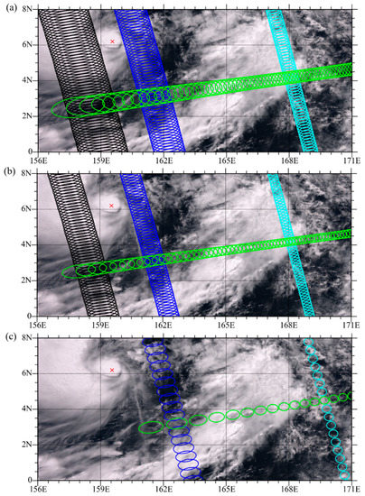
Figure 1.
(a) Advanced Technology Microwave Sounder Field Of View (ATMS FOV) footprints with a 5.2° beam width along the scan line whose nadir FOV was located at [169.1°E, 4.4°N] (green ovals), and the 2nd (black ovals, the scan angle from the nadir is 51.6°), 9th (blue ovals, the scan angle from the nadir is 44°), and 41st (cyan ovals, the scan angle from the nadir of 8.3°) scan lines in the along-track direction over a portion of the swath at the Suomi National Polar-orbiting Partnership (S-NPP) ascending node on 10 May 2015. The background image shows Visible Infrared Imaging Radiometer Suite (VIIRS) imager visible channel observations at 0210 UTC 10 May 2015. (b) Same as (a) except for the remapped ATMS FOVs at the 3.3° beam width. (c) Advanced Microwave Sounding Unit-A (AMSU-A) FOV footprints with a 3.3° beam width along the scan line whose nadir FOV was located at [169.1°E, 4.4°N] (green ovals), and the 2nd (blue ovals, the scan angle from the nadir is 44.6°) and 13th (cyan ovals, the scan angle from the nadir is 8.3°) scan lines in the along-track direction over a portion of the swath at the NOAA-19 ascending node on the same day as (a). The center of Typhoon Dolphin at this time was located at [159.56°E, 6.3°N] and is indicated by a red cross in (a–c).
The FOV sizes are significantly reduced after the remapping (Figure 1b). Such remapping from larger to smaller FOVs will increase the noise of the remapped ATMS observations. A remapped ATMS FOV overlaps with only two and three neighboring FOVs in the across-track and along-track directions, respectively. The remapped ATMS FOVs can be compared with the FOVs of NOAA-19 AMSU-A, whose equator crossing time is the closest to that of S-NPP. Figure 1c shows the FOV footprints of AMSU-A, whose beam width is 3.3°. The AMSU-A FOVs do not overlap along the scan line, whose nadir FOV was located at the same place as in Figure 1a,b. Only a very small overlap is found at large scan angles, such as the 2nd FOV, whose scan angle is 44.6°. Near the nadir, no overlap is found among the AMSU-A FOVs in the along-track direction, which is shown in Figure 1b for the 41st FOV at the 8.3° scan angle. Note that the ATMS swath width is wider than the AMSU-A swath width. Typhoon Dolphin’s center was covered by the ATMS swath but not by the AMSU-A swath in this case.
2.3. Diurnal Variation Calculation
The diurnal variation in LWP within a 24-h period, local time, at most geographical locations have a basic sinusoidal shape [2]. The diurnal variation can thus be estimated using the following equation [19,20]:
where is the mean LWP at a particular latitude (φ), longitude (λ), and local time t (unit: hours) estimated from data, and is the diurnal frequency. The amplitudes , , , , and are regression coefficients whose values are obtained by applying the least-squares fitting method to the LWP time series sampled at the local times of the AMSU-A/ATMS observations from NOAA-18/-19, MetOp-A/-B, and S-NPP. Note that the diurnal variations derived by Equation (4) represent the sum of the mean (), the 24-h diurnal cycle (), and the 12-h semi-diurnal cycle ().
3. Results of ATMS LWP Derived with and without the Remapping
In this study, the LWP values are calculated using the formula given by Weng et al. [21]. The LWP distribution derived from the ATMS BTs with the remapping seems similar to that without the remapping on a global map (figure omitted). A zoomed in look at the LWP distributions before and after remapping clearly shows the impact of the remapping on LWP. Figure 2 shows LWP distributions over the area defined by° [150°E–180°E, 10° S–15°N]. Since the remapping goes from a coarser resolution (5.2° beam width) to a higher resolution (3.3° beam width), the LWP in areas with the largest LWP values (>1.5 kg m−2) should and does become larger, i.e., on the order of 0.16–0.4 kg m−2. This may be related to the inhomogeneities caused by precipitation, most likely from deep convection.
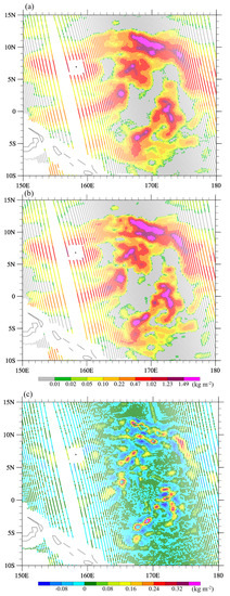
Figure 2.
Liquid water path (unit: kg m−2) calculated from (a) original S-NPP ATMS Temperature Data Records (TDRs), (b) remapped ATMS TDRs, and (c) differences [(b)–(a), or LWPRmp-LWPOri] at the ascending node on 10 May 2015.
Statistically examined next is the dependence of LWP differences between remapped (LWPRmp) and original (LWPOri) ATMS data on the magnitude of LWP. Figure 3 shows the mean values and standard deviations of LWP differences (i.e., LWPRmp–LWPOri) for all ATMS data from 9 to 15 May 2015, divided into three LWP groups: LWPori ≥ 1.5 kg m−2 (Figure 3a), 0.5 < LWPori ≤ 1.0 kg m−2 (Figure 3b), and 0.01 kg m−2 ≤ LWPori ≤ 0.5 kg m−2 (Figure 3c). The figure also shows data counts in 0.1-K Sea Surface Temperature (SST) and 0.01-kg-m−2 LWP difference interval boxes. The remapped LWP is ~0.1 kg m−2 larger than the LWP without remapping, on average (Figure 3a). The positive bias reduces to about 0.05 kg m−2 in the range of 0.5 < LWPori ≤ 1.0 kg m−2 (Figure 3b). The mean difference between the remapped and original LWPs is zero when 0.01 kg m−2 ≤ LWPori ≤ 0.5 kg m−2 (Figure 3c). This is because the smaller LWPs are little affected by the deconvolution since the scenes are relatively homogeneous at the spatial scale of the measurements. Note that the data counts are highest when LWP > 0.5 kg m−2 and SST is ~302 K (Figure 3a,b) and lowest when the SST ranges from 297.2 to 299.8 K (outlined by dashed lines in Figure 3a,b). When LWP ≤ 0.5 kg m−2, the data counts are high when SST ranges from 295 to 302 K (Figure 3c).
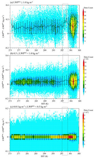
Figure 3.
Mean values (black curves) and standard deviations (black vertical lines) of LWP differences (i.e., LWPRmp–LWPOri) with respect to Sea Surface Temperature (SST) for (a) LWPOri ≥ 1.5 kg m−2, (b) 0.5 ≤ LWPOri < 1.0 kg m−2, and (c) 0.01 kg m−2 ≤ LWPOri ≤ 0.5 kg m−2 calculated from ATMS data from 9 to 15 May 2015. The LWP data counts (shaded in colors) are also shown at intervals of 0.1-K SST and 0.01-kg-m−2 LWP differences. The range of SST values from 297.2 to 299.8 K with nearly no large LWP values is outlined by dashed lines in (a,b).
Why is there a data gap of large LWP (>0.5 kg m−2) in regions of SST from 297.2 to 299.8 K? The latitudinal distribution of LWP data counts within 0.1-K SST/1°-latitude boxes for LWPori > 0.5 kg m−2 reveals that the May 2015 LWP data void was located in the subtropical latitudes. This data void is more noticeable in the Northern Hemisphere. The data counts for LWPori ≤ 0.5 kg m−2 in the subtropics are significantly smaller than in the tropics, but similar to those at higher latitudes. The slightly smaller number of LWP data counts over oceans in the middle latitudes of the Northern Hemisphere is due to the lesser extent of oceanic areas in this part of that hemisphere.
The LWPs retrieved from remapped ATMS brightness temperature observations are compared with the LWP from the TMI Level-2 hydrometeor product 2A12. A total of 120,022 ATMS measurements in January 2015 were collocated with TMI LWP retrieval data under the collocation criteria of less than a 15 min time difference and 50 km distance between these two sensors’ observations. Figure 4 shows a scatter plot of the collocated remapped ATMS-derived LWP and TMI LWP. It is found that the remapped ATMS LWP correlates well with those derived from TMI data. The Correlation Coefficient (CC) and Root-Mean-Square-Error (RMSE) are of 0.908 and 0.096 kg cm−2, respectively.
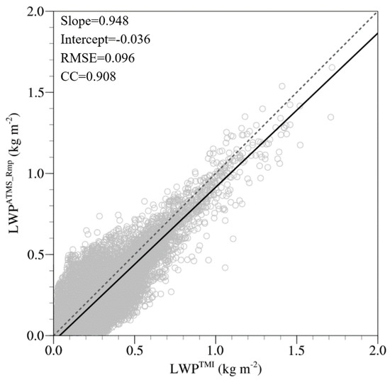
Figure 4.
Scatter plot of LWP over ocean from the remapped ATMS at ascending nodes versus collocated TMI LWP products in January 2015. The total number of collocated data points is 120,022.
4. Discussions on LWP When Merging S-NPP ATMS with Other Satellite Microwave Sounders
Before merging the AMSU-A-derived LWP data from different satellites, data are first inter-calibrated by a double difference method to remove inter-sensor biases [22]. Here, the AMSU-A data from NOAA-18 were used as the reference for the double difference inter-sensor calibration. The Local Equator Crossing Times (LECTs) for NOAA-18/-19, S-NPP, and MetOp-A/-B were 14:00, 14:00, 13:30, 09:30, and 09:30 Local Time (LT), respectively, right after their launch times. Atmospheric drag and gravity and satellite aging could cause orbit drifts, leading to changes in the LECT. By May 2015, the LECTs for NOAA-18/-19, S-NPP, and MetOp-A/-B were 17:00, 14:10, 13:30, 09:30, and 09:30 LT, respectively. The LECT of NOAA-19 is thus closest to that of S-NPP. Figure 5a shows the AMSU-A LWP distribution in the part of the AMSU-A swath that overlaps with the ATMS swath in the same small area shown in Figure 2. The collocation criteria between the AMSU-A onboard NOAA-19 and ATMS onboard S-NPP were set as the maximum time difference, less than 30 minutes, and the maximum spatial distance, less than 30 km. Except for the sparser distribution of points, the LWP distribution is comparable to the remapped ATMS LWP distribution (Figure 2b). The differences in LWP between the NOAA-19 AMSU-A and remapped ATMS vary between −0.12 and 0.36 kg m−2 (Figure 5b). In other words, the differences in LWP derived from remapped and original ATMS data (Figure 2c) are of similar magnitude as the differences in LWP derived from the AMSU-A and remapped ATMS data (Figure 5b), suggesting the importance of the ATMS remapping for establishing a long-term climate data record of LWP with the same 3.3° beam width. The discrepancy in LWP between the remapped ATMS and collocated AMSU-A retrievals is not absolute value dependent until the AMSU-A LWP exceeds ~1.5 kg m−2 (Figure 5c).
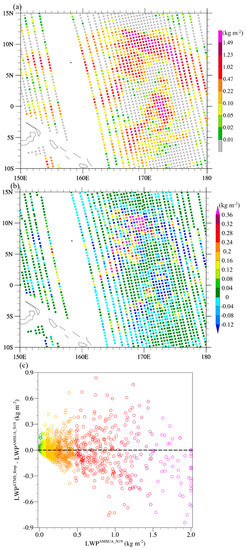
Figure 5.
(a) Liquid Water Path (LWP) (unit: kg m−2) from AMSU-A onboard National Oceanic Atmospheric Administration (NOAA)-19, (b) differences between NOAA-19 AMSU-A and remapped ATMS LWPs, and (c) differences between LWPATMS_Rmp and LWPAMSU-A (LWPATMS_Rmp - LWPAMSU-A) within the domain of 150°E –180° and 10° S–15°N at the ascending node on 10 May 2015. The color convention in (c) is the same as in (a).
A statistical evaluation of the differences in LWP due to remapping is provided in Figure 6, which includes all AMSU-A and ATMS data over the globe for January 2015. The mean difference is very small (~0.0016 kg m−2), suggesting that remapping introduced no bias. The standard deviation is also quite small (~0.014 kg m−2). Similar results are obtained for data in other months (figure omitted). Having demonstrated that there is no bias after remapping (Figure 6), we also confirmed that there is also no bias between collocated AMSU-A and remapped ATMS LWPs (Figure 7).
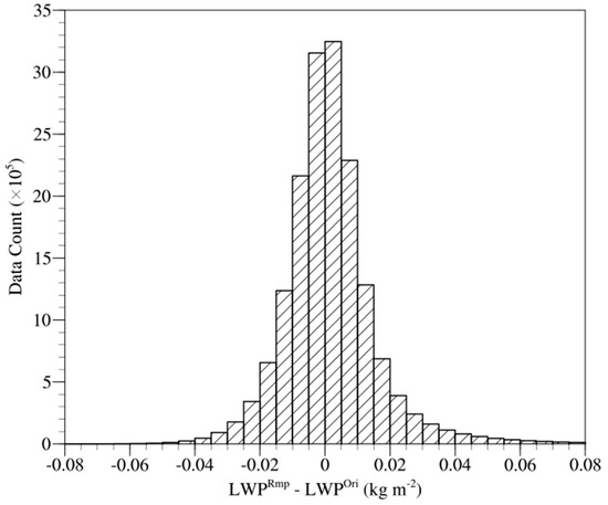
Figure 6.
Frequency distribution of the differences in LWP with and without the remapping (i.e., LWPRmp-LWPOri) for January 2015. The mean and standard deviation are 0.0016 kg m−2 and 0.014 kg m−2, respectively.
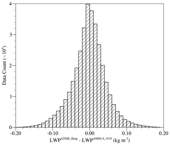
Figure 7.
Frequency distribution of the differences in LWP between the remapped ATMS and AMSU-A onboard N19 (i.e., LWPATMS_Rmp-LWPAMSUA_N19) for January 2015. The mean and standard deviation are −0.0022 kg m−2 and 0.046 kg m−2, respectively.
Figure 8 shows the monthly mean values and standard deviations of LWP derived from original and remapped ATMS data, as well as from NOAA-18/-19 and MetOp-A/-B AMSU-A data in 2015. Since the ATMS has a larger beam width than the AMSU-A, the standard deviations of LWP from the original ATMS data are the smallest and are significantly smaller than those of the AMSU-A-derived LWP. The ATMS remapping from a coarser to higher resolution significantly increases the mean values and standard deviations of LWP. ATMS LWP data after the remapping compared more favorably with the AMSU-A LWP data than before, although the LWP values retrieved by the remapped ATMS data remain lower than those from the AMSU-A data due to the larger beam width of the original ATMS channels 1 and 2.

Figure 8.
(a) Monthly mean values and (b) standard deviations of LWP from original (dashed blue) and remapped (solid blue) ATMS data, and data from AMSU-A onboard NOAA-19 (black), NOAA-18 (green), MetOp-A (orange), and MetOp-B (red) within 60° S-60°N over oceans in 2015.
The LWP over the Southeast Pacific Ocean has a well-known, well-defined diurnal variation [1,4,5]. A low-level stratiform cloud deck represents a significant mode of variability over the Southeast Pacific Ocean. This is an area without moderate to heavy precipitation, frozen particles, frequent deep convection, or widespread cirrus [2,23,24]. To illustrate that the LWP diurnal variations are derivable from the AMSU-A and ATMS data onboard five polar-orbiting satellites, Figure 9 shows the diurnal variations in LWP derived by Equation (4) from data at nadir (solid black curve), the western swath edge (blue dotted curve), and the eastern swath edge (red dashed curve) in the domain [85° W–82.5° W, 20° S–17.5° S] for March to April 2015 (Figure 9a) and November to December 2015 (Figure 9b). The reason for data from FOVs on the western edges of the ATMS swaths consistently yielding very different diurnal cycles than those at nadir and the eastern edges of the swaths is not clear and requires further study. The LWP curves derived from the S-NPP ATMS, NOAA-18/-19 and MetOp-A/-B AMSU-As at their local observing times over the Southeast Pacific Ocean are sinusoidal in shape, fit the observations quite well, and have peaks and valleys located at approximately 0400 LT and 1200–1600 LT, respectively. The fact that the diurnal cycle of LWP reaches its maximum and minimum values in the early morning and late afternoon is largely associated with solar absorption by stratiform clouds in this region. The amplitudes of the diurnal variations are generally small. We conclude that the AMSU-A/ATMS onboard these five polar-orbiting satellites (S-NPP, NOAA-18/-19, and MetOp-A/-B) captured the diurnal variation in LWP in 2015. Differences in diurnal variations of LWP among different FOVs are not negligible.
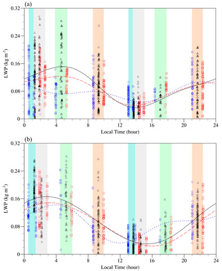
Figure 9.
LWP at the western swath edge (blue open circles), near nadir (black triangles), and the eastern swath edge (red open squares) from remapped ATMS data (blue-shaded columns) and AMSU-A data (NOAA-19: gray-shaded columns; NOAA-18: green-shaded columns; MetOp-A and MetOp-B: orange-shaded columns) over the eastern Pacific domain of [85° W–82.5° W, 20° S–17.5° S] in (a) March to April 2015 and (b) November to December 2015. The diurnal variations in LWP estimated from LWP data from all satellites at nadir, and at the western and eastern edges of the swath are shown by the black solid, blue dotted, and red dashed curves, respectively.
Figure 10 shows the bi-monthly mean diurnal cycles of LWP in 2015 over the Southeast Pacific Ocean. The diurnal cycle of LWP varies within the year. The amplitude of the diurnal cycle is the largest in November and December 2015, and the smallest in May and June 2015. Although the amplitudes of the diurnal cycle have a seasonal variability, the local times of the peaks and valleys of the diurnal variations in LWP over the Southeast Pacific Ocean, in all six bi-monthly periods, are similar. The diurnal cycle for the months of September and October 2015 has a second small peak around noon, which represents a slightly stronger semi-diurnal cycle over the eastern Pacific Ocean during September and October than during other months. Further research into these interesting differences in LWP diurnal variations among various months is warranted.
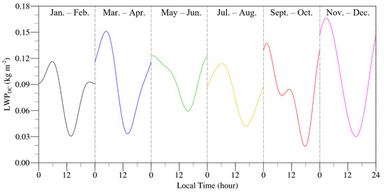
Figure 10.
Bi-monthly mean diurnal cycles of LWP at nadir in 2015 over the domain [85° W–82.5° W, 20° S–17.5° S].
5. Summary and Conclusions
AMSU-A instruments have been onboard the NOAA-15, -16, -17, -18, and -19 and the EUMETSAT MetOp-A, -B, and -C polar-orbiting satellites for some time. The AMSU-A and MHS were replaced by the ATMS following the launch of the NOAA satellite S-NPP in 2011. The ATMS onboard NOAA-20 launched in November 2017 and will also be onboard future JPSS satellites. Differences in beam width, data resolution, and FOV overlap between ATMS channels 1 and 2 and AMSU-A present new challenges for merging the ATMS LWP data with those from ATMS’ predecessor heritage AMSU-A instruments. This study first applies the remapping algorithm developed by Atkinson [13] to convert ATMS data to ATMS remapped data, which have the same beam width as AMSU-A observations. The redundant information contained in the ATMS neighboring overlapping FOVs makes it possible to remap the ATMS observations of channels 1 and 2 into a higher AMSU-A-like spatial observation resolution. The impacts of the remapping on the ATMS LWP retrievals are significant, especially in areas with large LWP. LWPs after the remapping are more consistent with AMSU-A-retrieved LWPs. The combination of LWP data from the NOAA-18/-19, S-NPP, and MetOp-A/-B satellites in 2015 captures well the diurnal variations in the western Pacific Ocean in the tropics. The diurnal cycle has maximum and minimum LWPs in the early morning (~0400 LT) and late afternoon (~1400–1600 LT), respectively. The semi-diurnal cycle has two maximum LWPs, one in the early morning (~0400 LT) and the other in the late afternoon (~1400–1600 LT). The intra-annual variability of the diurnal variations in LWP is mainly in amplitude, not the phase.
The remapping of ATMS data into AMSU-A-like data is a critical step towards linking ATMS data to NOAA and EUMETSAT AMSU-A time series to create a long-term fundamental climate data record of LWP. As more ATMS data from both S-NPP and NOAA-20 become available, results from the present study will be substantiated. We plan to generate the remapped ATMS LWP time series for the entire S-NPP ATMS eight-year time period (2012–2018) and merge it with the AMSU-A LWP time series to establish an ATMS/AMSU-A LWP climate data record from 1998 to the present. This dataset can then be used for climate monitoring, re-analysis, and climate prediction validation.
Moreover, it is worth noting that the two challenges of developing the LWP climate data records are validation and error characterization. Recent studies verified LWP retrieval with observations [25] and quantified the uncertainties of LWP retrieval [3,26,27], however, further investigation is still needed to investigate the complex uncertainty that largely depends on the retrieval algorithms [21,26,27].
Author Contributions
Conceptualization, methodology, investigation, X.Z. and L.L.; software, formal analysis, resources, data curation, L.L.; writing—original draft preparation, X.Z.; writing—review and editing, X.Z. and L.L.; project administration and funding acquisition, L.L. and X.Z. All authors have read and agreed to the published version of the manuscript.
Funding
This research was supported by NOAA grant NA14NES4320003 and NA19NES4320002 (Cooperative Institute for Satellite Earth System Studies-CISESS) at the Earth System Science Interdisciplinary Center (ESSIC), University of Maryland for the first author, and by the National Key R&D Program of China grant 2018YFC1507004 for the corresponding author.
Acknowledgments
The authors would like to acknowledge all STAR colleagues for their input during the process of conducting this research.
Conflicts of Interest
The authors declare no conflicts of interest.
References
- Wood, R.; Bretherton, C.S.; Hartmann, D.L. Diurnal cycle of liquid water path over the subtropical and tropical oceans. Geophys. Res. Lett. 2002, 29, 7-1–7-4. [Google Scholar] [CrossRef]
- O’Dell, C.W.; Wentz, F.J.; Bennartz, R. Cloud liquid water path from satellite-based passive microwave observations: A new climatology over the global ocean. J. Clim. 2008, 21, 1721–1739. [Google Scholar] [CrossRef]
- Elsaesser, G.S.; O’Dell, C.W.; Lebsock, M.D.; Bennartz, R.; Greenwald, T.J.; Wentz, F.J. The multisensor advanced climatology of liquid water path (MAC-LWP). J. Clim. 2017, 30, 10193–10210. [Google Scholar] [CrossRef]
- O’Neill, L.W.; Wang, S.; Jiang, Q. Satellite climatology of cloud liquid water path over the Southeast Pacific between 2002 and 2009. Atmos. Chem. Phys. Discuss. 2011, 11, 31159–31206. [Google Scholar]
- Zou, X.; Weng, F.; Zhang, B.; Lin, L.; Qin, Z.; Tallapragada, V. Impact of ATMS radiance data assimilation on hurricane track and intensity forecasts using HWRF. J. Geophys. Res. Atmos. 2013, 118, 11558–11576. [Google Scholar] [CrossRef]
- Zou, X.; Qin, Z.; Weng, F. Impacts from assimilation of one data stream of AMSU-A and MHS radiances on quantitative precipitation forecasts. Q. J. Roy. Meteor. Soc. 2017, 143, 731–743. [Google Scholar] [CrossRef]
- Spencer, R.W.; Christy, J.R.; Grody, N.C. Global atmospheric temperature monitoring with satellite microwave measurements: Method and results 1979–1984. J. Clim. 1990, 3, 1111–1128. [Google Scholar]
- Weng, F.; Zou, X. 30-year atmospheric temperature trend derived by one-dimensional variational data assimilation of MSU/AMSU-A observations. Clim. Dynam. 2014, 43, 1857–1870. [Google Scholar] [CrossRef]
- Zou, X.; Qin, Z.; Weng, F. Improved quantitative precipitation forecasts by MHS radiance data assimilation with a newly added cloud detection algorithm. Mon. Weather Rev. 2013, 141, 3203–3221. [Google Scholar] [CrossRef]
- Qin, Z.; Zou, X. Development and evaluation of a new index for MHS cloud detection over land. J. Meteor. Res. 2016, 30, 12–37. [Google Scholar] [CrossRef]
- NOAA KLM User’s Guide, Section 3.3. National Oceanic Atmospheric Administration: Washington, DC, USA. Available online: https://www1.ncdc.noaa.gov/pub/data/satellite/publications/podguides/N-15%20thru%20N-19/pdf/0.0%20NOAA%20KLM%20Users%20Guide.pdf (accessed on 26 May 2020).
- Weng, F.; Zou, X.; Sun, N.; Blackwell, W.J.; Leslie, V.; Yang, H.; Wang, X.; Lin, L.; Tian, M.; Mo, T. Calibration of Suomi National Polar-Orbiting Partnership (NPP) Advanced Technology Microwave Sounder (ATMS). J. Geophys. Res. Atmos. 2013, 118, 11187–11200. [Google Scholar] [CrossRef]
- Atkinson, N.C. NWP SAF Annex to AAPP scientific documentation: Pre-processing of ATMS and CrIS Version 1.0. 2011, EUMETSAT Satellite Application Facility on Numerical Weather Prediction (NWP SAF). The European Organisation for the Exploitation of Meteorological Satellites (EUMETSAT). Available online: https://www.nwpsaf.eu/site/download/documentation/aapp/NWPSAF-MO-UD-027_ATMS_CrIS.pdf (accessed on 26 May 2020).
- Sorensen, H.; Jones, D.; Heideman, M.; Burrus, C. Real-valued fast Fourier transform algorithms. IEEE Trans. Acoust. Speech Signal. Process. 1987, 35, 849–863. [Google Scholar] [CrossRef]
- Bormann, N.; Bell, W.; Fouilloux, A.; Ioannis, M.; Atkinson, N.; Swadley, S. Initial results from using ATMS data at ECMWF. In Proceedings of the 18th International TOVS Study Conference, Toulouse, France, 21–27 March 2012; Available online: http://cimss.ssec.wisc.edu/itwg/itsc/itsc18/program/files/links/1.17_Bormann_pa.pdf (accessed on 19 June 2020).
- Doherty, A.; Atkinson, N.; Bell, W.; Smith, A. An assessment of data from the advanced technology microwave sounder at the Met Office. Adv. Meteorol. 2015, 2015, 956920. [Google Scholar] [CrossRef]
- Zhu, Y.; Gayno, G.; Purser, R.J.; Su, X.; Yang, X. Expansion of the all-sky radiance assimilation to ATMS at NCEP. Mon. Weather Rev. 2019, 147, 2603–2620. [Google Scholar] [CrossRef]
- Zhou, J.; Hu, Y. Comparison of the Remapping Algorithms for the Advanced Technology Microwave Sounder (ATMS). Remote Sens. 2020, 12, 672. [Google Scholar] [CrossRef]
- Tang, F.; Zou, X. Diurnal variation of liquid water path derived from two polar-orbiting FengYun-3 microwave radiation imagers. Geophys. Res. Lett. 2018, 45, 6281–6288. [Google Scholar] [CrossRef]
- Chen, H.; Zou, X.; Qin, Z. Effects of diurnal adjustment on biases and trends derived from inter-sensor calibrated AMSU-A data. Front. Earth Sci. 2018, 12, 1–16. [Google Scholar] [CrossRef]
- Weng, F.; Zou, X.; Wang, X.; Yang, S.; Goldberg, M.D. Introduction to Suomi NPP ATMS for NWP and tropical cyclone applications. J. Geophy. Res. Atmos. 2012, 117, 1–14. [Google Scholar]
- Xia, X.; Zou, X. Impacts of AMSU-A inter-sensor calibration and diurnal correction on satellite-derived linear and nonlinear decadal climate trends of atmospheric temperature. Clim. Dynam. 2020, 54, 1245–1265. [Google Scholar] [CrossRef]
- Minnis, P.; Harrison, E.F. Diurnal variability of regional cloud and clear-sky radiative parameters derived from GOES data. Part I: Analysis method. J. Appl. Meteor. 1984, 23, 993–1011. [Google Scholar] [CrossRef]
- Garreaud, R.D.; Munoz, R. The diurnal cycle in circulation and cloudiness over the subtropical southeast Pacific: A modeling study. J. Clim. 2004, 17, 1699–1710. [Google Scholar] [CrossRef]
- Painemal, D.; Greenwald, T.; Cadeddu, M.; Minnis, P. First extended validation of satellite microwave liquid water path with ship-based observations of marine low clouds. Geophys. Res. Lett. 2016, 43, 6563–6570. [Google Scholar] [CrossRef]
- Lebsock, M.; Hui, S. Application of active spaceborne remote sensing for understanding biases between passive cloud water path retrievals. J. Geophy. Res. Atmos. 2014, 119, 8962–8979. [Google Scholar] [CrossRef]
- Greenwald, T.J.; Bennartz, R.; Lebsock, M.; Teixeira, J. An uncertainty data set for passive microwave satellite observations of warm cloud liquid water path. J. Geophy. Res. Atmos. 2018, 123, 3668–3687. [Google Scholar] [CrossRef] [PubMed]


© 2020 by the authors. Licensee MDPI, Basel, Switzerland. This article is an open access article distributed under the terms and conditions of the Creative Commons Attribution (CC BY) license (http://creativecommons.org/licenses/by/4.0/).