1. Introduction
Ecosystems of mixed herbaceous and woody vegetation cover over one fifth of the Earth’s surface [
1], supporting significant global biodiversity and wildlife habitat as well as providing ecosystem services such as water and soil conservation and livestock grazing [
2,
3,
4,
5,
6]. The woody vegetation in these environments, often dominated by shrub species, also plays an important role in the global carbon cycle [
6,
7], storing up to 30% of global terrestrial carbon in above- and belowground biomass [
8]. The ability of shrubs to store carbon, produce food for wildlife and livestock, and provide ecosystem services is closely linked to their distribution, physical structure, and biomass. These characteristics are dynamic across space and time and increasingly impacted by human development and climatic changes [
1,
7,
9,
10,
11]. In some shrub-dominated environments, the number, size, and distribution of shrubs is decreasing [
10,
12,
13,
14], potentially impacting the ecosystem services and interactions they bestow [
15,
16]. In other environments, the encroachment of shrubs into previously-unoccupied ecosystems presents a conservation concern [
17,
18,
19,
20].
However, there has been less focus on modelling aboveground biomass (AGB) in shrub-dominated ecosystems compared to environments such as forests. It is more difficult to accurately characterize low-stature vegetation [
21] and there is less economic interest in shrubs [
22], which are considered unwanted “nuisance species” in some areas [
17,
23]. As a result, efficient methods for measuring and monitoring shrub biomass across ecosystems are relatively poorly developed.
It can be challenging to characterize shrub AGB with conventional remote sensing methods because shrub-dominated vegetation communities tend to be spatially heterogeneous at fine scales, spectrally indistinct, and low in stature [
6,
7,
15]. However, in recent years there has been an increase in the use of unmanned aerial systems (UASs) as remote-sensing platforms [
24,
25,
26,
27,
28,
29]. A significant advantage of UAS-based remote sensing is the ability to simultaneously collect very high-resolution data on the structural and spectral characteristics of vegetation at scales suitable for detecting small or low-growing plants [
5,
30,
31,
32,
33]. Despite a demonstrated ability of UAS data to estimate the fine-scale AGB of vegetation including arable and non-arable crops [
26,
32,
33,
34,
35,
36,
37,
38,
39], trees [
28,
31,
40,
41,
42,
43], mangrove and wetland plants [
44,
45,
46], and grasses [
2,
5,
47,
48], comparatively few studies have used UAS data for shrub biomass estimation. For example, Cunliffe et al. [
9] found that structural metrics of shrub height derived from a canopy height model (CHM) could accurately estimate shrub AGB in a dryland ecosystem in the southwestern USA. The opportunity thus exists to more broadly explore the use of UAS-derived data for determining the biomass of shrub species in other ecosystems and to test which data type(s) (i.e., spectral, structural) are most accurately able to estimate shrub AGB.
In many rangeland environments, including shrublands, large ungulate grazers and periodic fires have historically played significant roles in shaping vegetation community structure and biodiversity [
49]. The frequency and intensity of these disturbances are critical to habitat heterogeneity and ecological processes at multiple spatial scales [
50]. However, most rangeland management practices have been developed to increase livestock production and favour a few key forage species rather than promote a heterogeneous distribution of vegetation across the landscape [
51]. Restoring the natural ecological function of grazers and managing rangelands for heterogeneity is increasingly recognized as a key component of successful large-scale conservation of biodiversity and ecosystem integrity in rangelands [
51,
52,
53].
With this goal in mind, plains bison (
Bison bison bison) were reintroduced in 2018 to Banff National Park in Canada, a region bison have been absent from since their extirpation in the 1800s [
54]. Plains bison play a keystone role in ecosystems, impacting and altering vegetation communities through browsing, grazing, roaming, and wallowing [
55]. Efficient and accurate methods of monitoring the distribution and abundance of vegetation in the region occupied by the newly reintroduced bison are needed to support park management and quantify their impact on the ecosystem. The fine spatial and temporal resolution of bison-vegetation dynamics makes the use of either ground-based or traditional aerial remote sensing for detecting these processes challenging. However, it is an ideal setting to investigate whether UAS imagery can be used to estimate and track changes in shrub AGB and distribution over time as bison occupy this landscape once again.
Our overall objective in the work reported in this manuscript was to develop a workflow for estimating shrub AGB using data collected from UAS surveys. To achieve that, we sought to answer the following primary research questions: (i) which structural and/or spectral variables have the highest correlations with allometric AGB, (ii) which structural and/or spectral variables best predict allometric AGB in regression models, and (iii) are the best AGB estimation models robust enough to be applied to another spatially distinct location? In addition to these primary research questions, we had a set of secondary follow-up questions: (i) are the remote-sensing models sensitive enough to detect simulated ungulate browsing of shrubs and (ii) what is the total shrub aboveground biomass across the study site? While this study was conducted within the context of bison reintroduction to Banff National Park, our methods and results are informative for researchers interested in developing similar models of shrub biomass from UAS data in other rangeland ecosystems or for other ecological applications.
2. Materials and Methods
2.1. Study Area
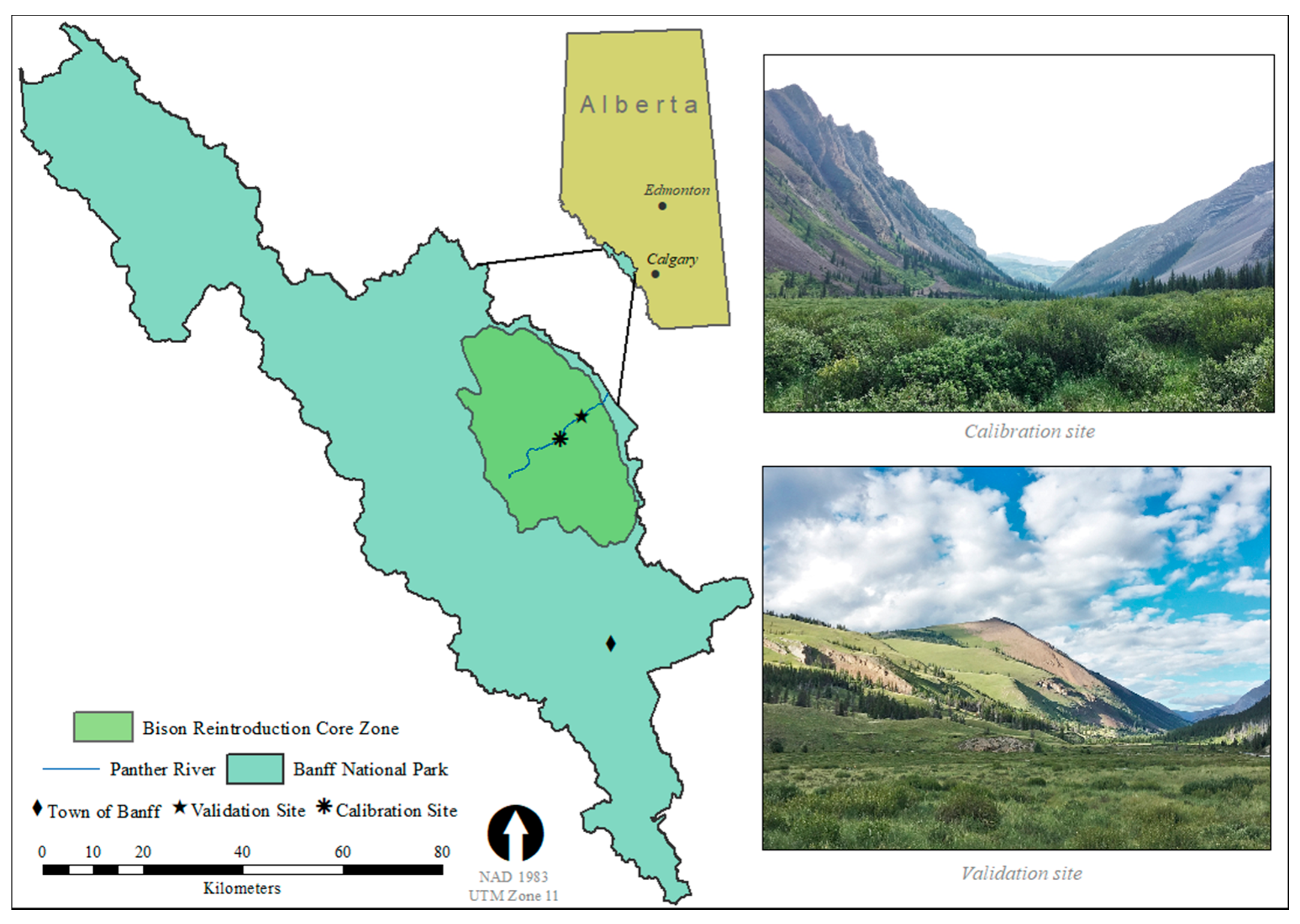
Our fieldwork was conducted within the Panther River Valley in Banff National Park in the Rocky Mountains of Alberta, Canada (
Figure 1). This area was determined to have the highest carrying capacity and best habitat suitability for bison within the park due to current habitat conditions and past evidence of bison occupation [
54]. Banff National Park was established as a protected region in 1885 and has an area of 6641 km
2. The park is characterized by its climate of short, dry summers and long cold winters as well as its extremely mountainous terrain, broken up by large valleys 2–5 km wide [
54]. The Panther River is shallow throughout its gravel bed and flows in a north-easterly direction from its headwaters towards the eastern boundary of the park. Common vegetation in the river valley includes intermittent stands of Douglas fir (
Pseudotsuga menziesii), white spruce (
Picea glauca), and aspen (
Populus tremuloides) interspersed with open grasslands with abundant forbs, graminoids, and shrubs including species of the
Betula (birch) and
Salix (willow) genera [
56].
2.2. Site and Plot Selection
We conducted our fieldwork at two different sites within the Panther River Valley located approximately 40 km north of the Banff town site (
Figure 1). The first site (calibration site) was where all destructive ground-based sampling took place. This site was selected due to the abundance and diversity of sizes of shrubs in the
Betula and
Salix genera, lack of hazards for UAS flying, and proximity to a warden cabin for logistics. The second site (validation site) was located 6.6 km northeast of the calibration site along the Panther River and was selected due to its similar vegetative characteristics and geographic separation from the calibration site.
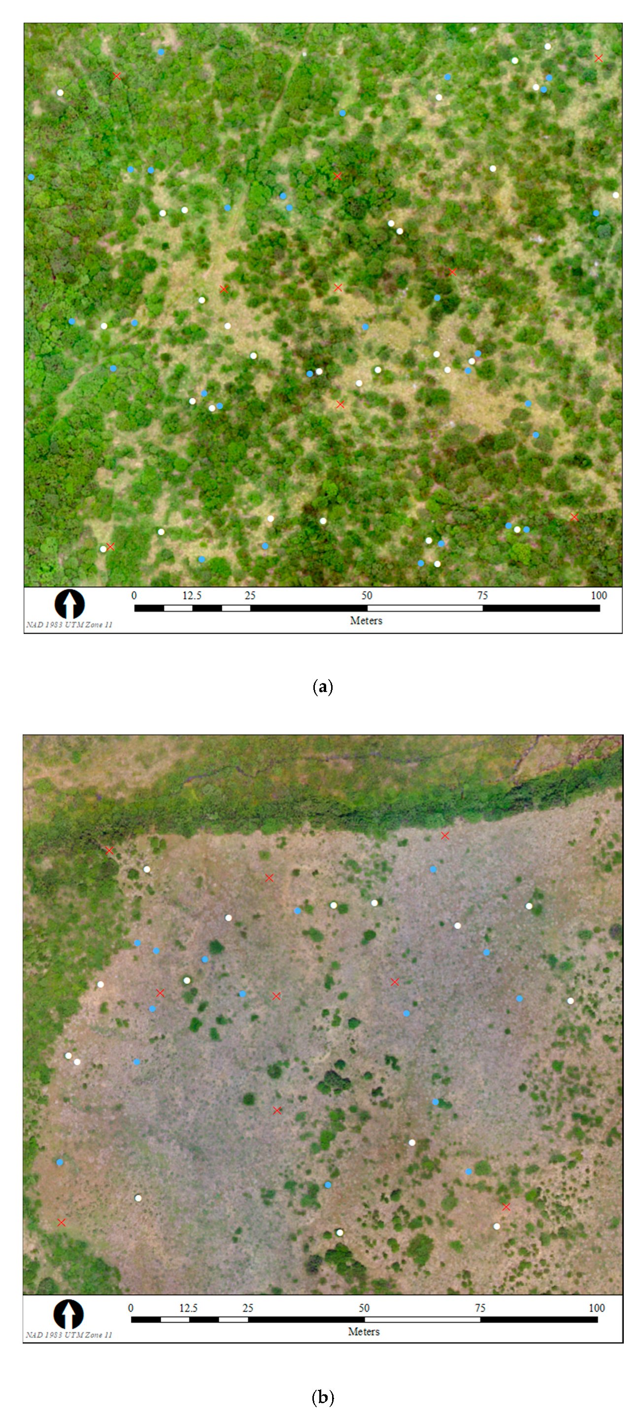
At the calibration site, we selected individual shrubs for destructive sampling (
Figure 2a) using a multi-stage sampling strategy comprised of a systematic primary stage and stratified-random secondary stage. In the primary stage, we started at the west end of each of five 125-m long transects across the study site and progressed eastward using a compass and GPS. On each transect we stopped every 20 m to locate a set of “suitable” shrubs: individuals reasonably distinct from their neighbours so that they could be removed cleanly during sampling. At each measurement point along the transect we marked the nearest three suitable shrubs in each of the
Betula and
Salix genera and recorded the GPS location, size (small, medium, or large relative to other shrubs), and genus of each shrub using a Hemisphere S320 GPS unit with ~10 mm horizontal precision. After the five transects were complete, we had obtained a potential sampling pool of 90 shrubs of each genus. In the secondary stage, we selected 30 shrubs of each genus using a stratified-random approach: 10 shrubs randomly selected from each of the strata of small, medium, and large size classes.
At the validation site the sampling was non-destructive, so it was particularly important that each shrub be distinct from its neighbours to ensure we would only measure stems of that shrub during sampling and that the outline of each shrub would be obvious in aerial imagery. At each of the centre, northeast, northwest, southeast, and southwest ground control point (GCP) locations, we observed the nearest shrubs of each genus and selected one of each size class (small, medium, and large) of suitable, distinct
Salix and
Betula shrubs for non-destructive sampling (
Figure 2b), resulting in a sample of 15 of each genera of shrub, five in each size class.
2.3. Ground-Based Biomass Data Collection and Allometric Equations
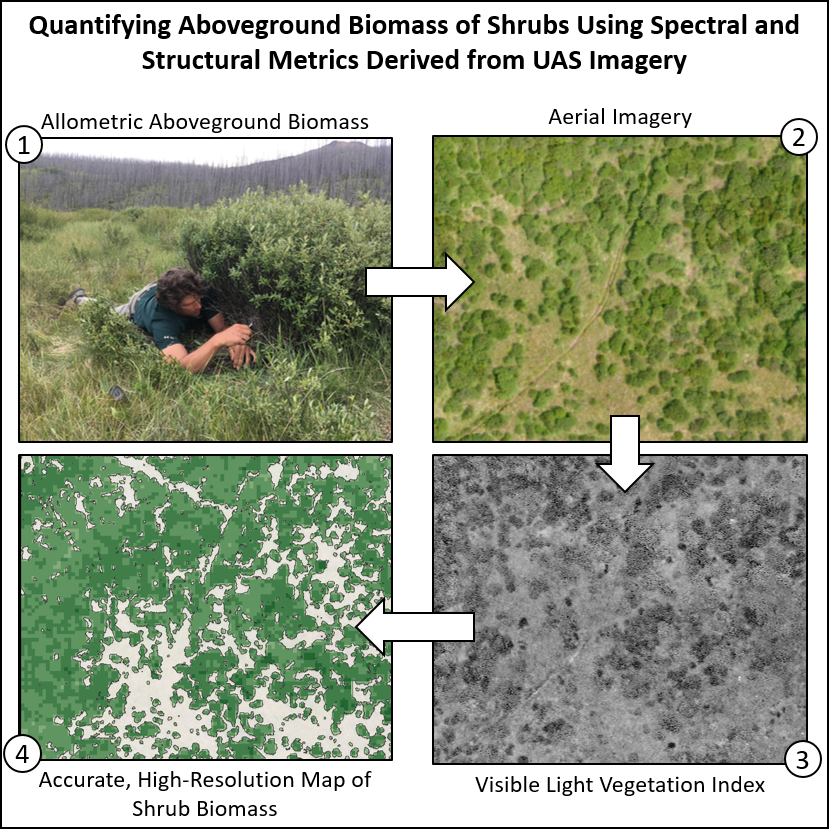
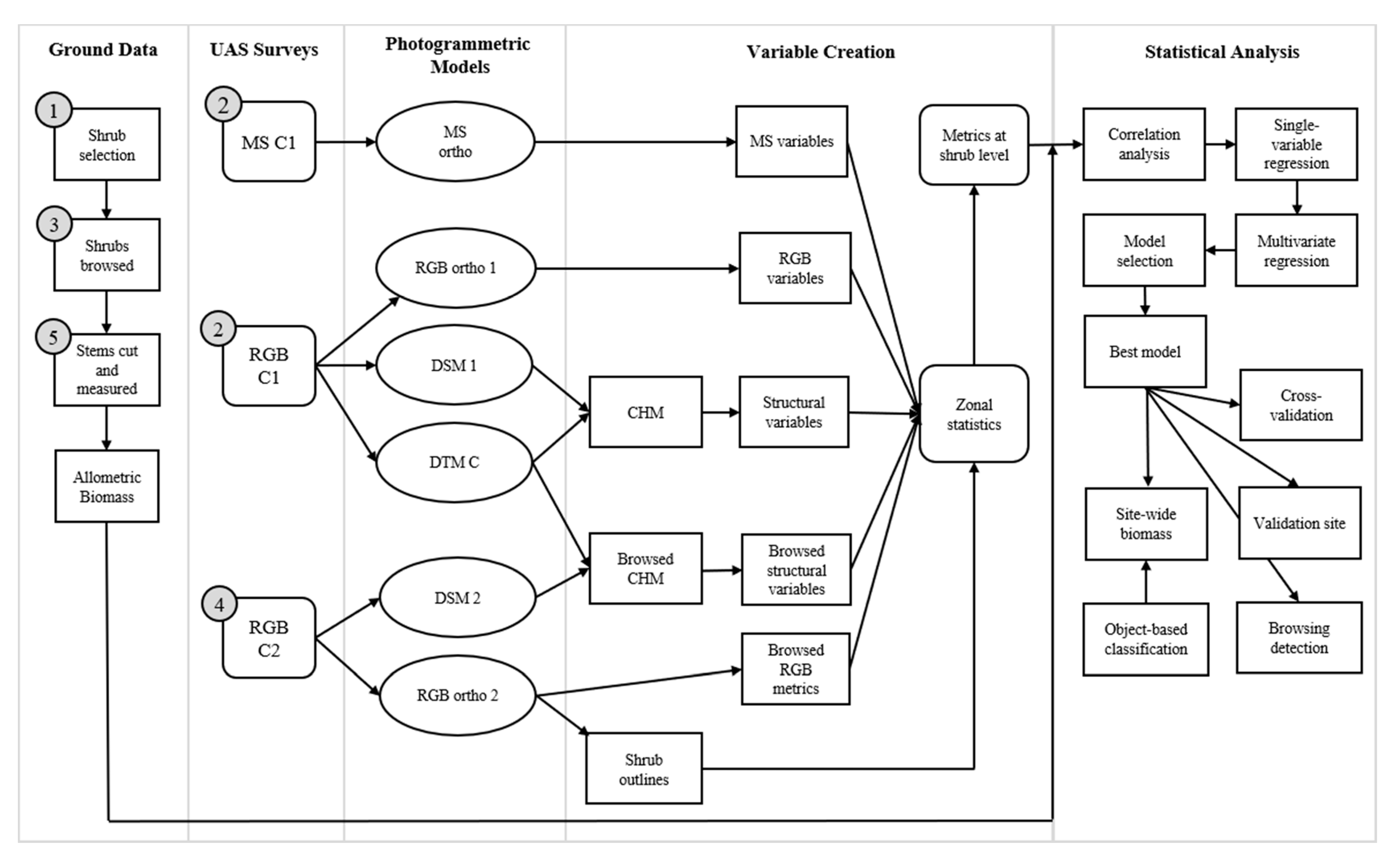
Figure 3 shows the order of steps taken during the data collection and analysis workflow used in this study. At the calibration site we collected ground-based measurements of shrub biomass in July 2018. After sample shrubs were selected (number 1 in grey circle in
Figure 3), we conducted one visible light (RGB) and one multispectral (MS) UAS survey of the calibration site (2). Then, we simulated ungulate browsing by trimming the leaves and terminal ends of stems off each shrub in the sample (3) and conducted an RGB survey of the site with the browsed shrubs clearly marked in the imagery (4). Lastly, we cut each stem at the base ensuring that we did not cut below the soil level. We recorded the basal stem diameter (BSD) in mm and the number of stems of each shrub we removed (5).
At the validation site, we flew one RGB and one MS survey prior to taking any measurements. Next, we measured the BSD in millimetres of every stem of each selected Betula and Salix shrub without removing any stems. Flagging tape in the same patterns as at the calibration site, laid over the top of each measured shrub, was used to indicate shrub genus and location, and we conducted a final RGB survey to collect images with shrub markers.
Allometric equations for shrub AGB estimation derived previously in our study area [
57] were used to estimate shrub AGB. Models have an exponential form (y = ae
bx) where y is biomass (g) and x is the basal stem diameter (mm). We used the allometric equations to estimate leaf biomass (a = 6.3794, b = 0.0918) and twig biomass (a = 12.282, b = 0.0854) for each measured stem in each shrub from the BSD measurements, then summed the biomass for all stems in the shrub to get a measure of leaf, twig, and total aboveground biomass in grams for each shrub.
2.4. UAS Surveys
UAS surveys were conducted using the senseFly eBee fixed-wing UAS equipped with two different sensors. The S.O.D.A. sensor collects three-band RGB imagery with a resolution of 20 MP. The Sequoia four-band multispectral sensor simultaneously collects four images with 1.2 MP resolution using a rolling shutter in four wavelengths: green (550 ± 40 nm), red (660 ± 40 nm), red edge (735 ± 10 nm), and near infrared (790 ± 40 nm). The Sequoia includes a “sunshine sensor” to collect information on incoming solar irradiance used to correct imagery collected under different illumination conditions as well as a target used in post-processing to calibrate imagery to ambient lighting conditions [
58].
Prior to each survey, nine ground control points (GCPs) were placed across the site. The markers were staked to the ground through the centre using magnetic survey pins to a height of five centimetres above the ground to ensure GCPs were placed at the exact same position each survey. At both sites, GCP placement followed the same pattern: one in the centre of the site, one each at ~25 m from the centre GCP to the north, east, south, and west, and one each at ~50 m from the centre GCP to the northeast, northwest, southeast, and southwest.
Survey flights were planned in the mission planning software eMotion 3 (senseFly, Cheseuax-sur-Laussane, Switzerland). Surveys were designed so that the UAS flew in a grid pattern over the site, flying a series of parallel transects and then another series of transects at a 90° angle to the first set. Overlap between photos on the same transect was 70%, and the overlap between photos on adjacent transects (sidelap) was 80%, with a height above take off point of 70 m for all flights, resulting in an average ground sample distance (GSD) of 1.5 cm in the RGB imagery and 6 cm in the multispectral imagery. A total of six survey flights were conducted: three at the calibration site and three at the validation site (
Table 1). Following the survey flights, we downloaded the aerial imagery and UAS flight logs and geotagged images using eMotion 3 with GPS locations recorded when each photo was taken by the UAS’s autopilot.
2.5. UAS Imagery Processing
We processed images from the S.O.D.A. RGB sensor using Agisoft PhotoScan version 1.4. This software uses a structure from motion (SfM) algorithm to identify features appearing in multiple images and generate 3D models and orthomosaics from a series of overlapping photos [
59,
60].
Our workflow in PhotoScan to process each set of RGB images and produce photogrammetric point clouds and georeferenced orthomosaics was as follows: first, we filtered out low-quality photos by examining each photoset and deleting any photos that were extremely blurry or had very different illumination from other photos. Then, we used the Align Photos tool to find tie points common in images and create a sparse point cloud, followed by the Build Dense Cloud tool to create a dense 3D point cloud. Each point cloud was georeferenced using the ground-measured GPS coordinates of the nine ground control markers, and then, the Optimize Alignment tool was used to improve the sparse point cloud based on the identified coordinates. We used the Build Mesh tool to create a 3D mesh surface, the Build Texture tool to create a texture file for the surface, and the Build Orthomosaic tool to create a georeferenced seamless orthomosaic from each photoset and to export each orthomosaic. Lastly, a Digital Surface Model and a Digital Terrain Model were created by classifying ground points in the point cloud and using the Build DEM tool to export a surface both with all points (DSM) and excluding non-ground points and extrapolating the surface where points were excluded (DTM).
For the multispectral imagery, we used Pix4D version 4.5.2 for data processing and orthomosaic creation as we found its procedure for calibrating multispectral imagery produced superior results compared to PhotoScan. Prior to processing, we ensured each of the four bands were radiometrically calibrated using the built-in radiometric calibration workflow included in the Pix4D software for calibration of multispectral imagery from the Sequoia sensor. This workflow uses data from the camera’s sunshine sensor and from the calibration target that was imaged prior to each survey in order to correct and calibrate the images’ reflectance values according to the known values on the calibration target. Following this, the “Ag Multispectral” processing template from Pix4D’s options was used to run the “Initial Processing” step using the default options in order to create a sparse point cloud. We used the rayCloud editor to georeference the point clouds using the GPS locations of the GCPs followed by the “Reoptimize” step to realign the sparse point cloud using the known GCP locations. Finally, we ran steps 2 (Point Cloud and Mesh) and 3 (DSM, Orthomosaic, and Index) using the default options to produce dense point clouds, DSMs, and orthomosaics for each of the four multispectral bands.
After all the RGB and multispectral datasets were processed, we used the high-resolution orthomosaics, which clearly showed shrub boundaries and flagging tape marking all measured shrubs in the study area, to manually delineate the outline of each measured shrub in ArcMap version 10.5 at the validation and calibration sites.
2.6. Structural and Spectral Variable Derivation
We used an area-based approach to derive spectral and structural metrics at the level of each individual shrub. The area-based approach was chosen because our ground-based biomass data was collected at the scale of individual shrubs. Three different types of variables within the outline of each measured shrub were created: structural variables, representing attributes of the shrub related to height and canopy volume; spectral variables derived from the RGB imagery; and spectral variables derived from the multispectral imagery. We then calculated statistical metrics for each variable representing measures of central tendency, range, and variability of values within each measured shrub.
Using the digital surface and digital terrain models from our surveys (
Table 1) we created canopy height models (CHMs) from which structural shrub attributes could be measured. First, we imported the DSMs, DTMs, and orthomosaics from each flight into ArcMap where they were displayed as raster imagery with each point having an x, y, and z value. With the Raster Math tool in ArcMap, we created a CHM by subtracting the values of the DTM from the values of the DSM at each point, resulting in another raster where each point has the same x and y values as the input rasters but a z value representing the difference in height between the DSM and the DTM. We created two CHMs at the calibration site, one with shrubs un-browsed (DSM1 − DTM C) and one with shrubs browsed (DSM2 − DTM C), and one CHM at the validation site (DSM V − DTM V). The un-browsed shrub CHM was used for most of the analysis at the calibration site, while the browsed shrub CHM was used only to examine whether changes in shrub AGB due to browsing could be detected. We then used the Zonal Statistics tool in ArcMap on each CHM to calculate maximum height, mean height, and shrub volume (the sum of all z-values within the shrub;
Table 2).
Using the orthomosaics created from the RGB and multispectral imagery we derived a series of single-band metrics or multi-band vegetation indices (VIs) for each shrub. We reviewed existing studies using RGB and/or multispectral data derived from UAS imagery to estimate vegetation biomass to see which indices and wavelengths have previously been useful for this application and selected 28 RGB and 6 multispectral indices for their ability to accurately estimate shrub biomass (
Table 2). For the single-band variables, we used Zonal Statistics as Table tool to calculate statistics for each of the four multispectral and three RGB bands within the outline of each measured shrub. For RGB and multispectral indices using two or more bands, we used the Image Analysis window in ArcGIS to calculate the index based on the formula found in the literature. We then used the Zonal Statistics as Table tool to calculate statistics on each index within the outlines of the measured shrubs. For all spectral variables, we calculated six basic descriptive statistics for each shrub: minimum value, maximum value, range, mean value, standard deviation, and sum of all values.
2.7. Shrub Biomass Model Creation and Selection
We conducted the following statistical analyses in SPSS version 26 (IBM, Armonk, NY, USA). Using a stepwise approach, we derived a candidate set of single- and multiple-variable linear regressions using a stepwise approach to ensure only significant variables were retained in models. First, we conducted a single-variable linear regression analysis using each of the metrics as the predictor variable and allometric biomass as the dependent variable. Then, a set of models with two predictor variables was created by combining two variables at a time, and it was evaluated whether model fit was improved over single-variable models. Lastly, we tested whether adding in a third variable, again selected from the top single-variable models, to the best two-variable models could improve performance. Correlations among all predictor variables were assessed prior to model building (
Appendix A,
Table A1), and variance inflation factor (VIF) values between predictor variables were examined in regression model outputs. Variables with correlations >0.50 or VIF values >2 were not included in the same model to avoid issues of collinearity in regression models, which can affect the slope and/or significance of predictor parameter estimates [
71].
Several methods were used to assess model fit to determine which combination of the derived parameters most accurately estimated shrub biomass in the best models containing uncorrelated predictor variables. We compared the coefficient of determination (R
2) statistic for each model. We also used the Akaike’s information criterion (AIC) approach to model selection. AIC is useful for finding the most parsimonious model that best fits the data within an a priori candidate set of models [
72]. Since our sample size was small (60), the number of parameters in each model divided by the number of samples (n/
K) was less than 40, so we used the corrected AIC statistic (AICc) for small sample sizes, with lower values indicating better model fit to the data as compared to other models in that candidate set [
72]. We compared the Δi values for each model, which indicate the increase in AICc value of each model compared to the model with the lowest AICc, and the model weight, which indicates the strength of support for that model being the most appropriate among the candidate set of models. Lastly, we looked at the standard error (SE) and significance for predictor variable parameter estimates, excluding models that did not have significance (
p-value > 0.05 or parameter estimate confidence interval overlapping zero) in at least 50% of the predictor variables from the AIC model selection.
2.8. Shrub Biomass Model Validation
We applied each of the selected models developed at the calibration site to predict biomass of shrubs at the validation site to evaluate how well each model performed at a geographically distinct location from the training site. We used the parameter estimates from each top model equation to estimate biomass for each of the 15 Betula and 15 Salix shrubs measured at the validation site, then conducted a linear regression between the predicted and the observed biomass for each shrub.
We used the coefficient of determination values from the linear regressions using UAS-derived biomass to predict allometric biomass to assess validation model performance and compared the root mean square error (RMSE) and mean absolute error (MAE) statistics averaged across the testing folds of each model, with lower values of these two statistics indicating less difference between predicted and observed biomass. We also calculated the mean bias error (MBE) for the validation site biomass estimates, where values close to zero indicate no bias in predicted biomass, positive values indicate biomass is overestimated on average, and negative values indicate biomass is underestimated.
2.9. Mapping Shrub Biomass Across the Study Area
In order to estimate site-wide shrub biomass, we classified the study area using the rule-based, object-oriented feature extraction tool in the software ENVI version 5.5 (L3Harris, Melbourne, FL, USA). We applied our classification using three raster images as input data that we found were most useful for distinguishing between shrub and non-shrub objects: the CHM, the BGRI vegetation index, and the red ratio vegetation index. Following segmentation, we defined rules for three classes: shrubs, grass, and other, which included dead trees, small rocks, and gravel. The result of the classification was a shapefile with the boundaries of each of the three classes, which we imported into ArcGIS version 10.7 (ESRI, Redlands, CA, USA).
To assess classification accuracy, we generated 200 points distributed randomly across the image and visually determined the true class and rule-based class each point fell within. We then used a confusion matrix to calculate errors of omission and commission and producer’s and user’s accuracy for each class (
Appendix B,
Table A2). Out of the 200 random points generated, 193 were assigned to the correct class, giving a total accuracy of 0.965. The shrub class had a producer’s accuracy of 0.99 and a user’s accuracy of 0.97 with slightly more errors of commission than omission.
We created a 1 × 1-m grid covering the classified shrub area to display shrub biomass at a fine scale. Then, we extracted the total sum of VI and CHM values in each grid cell across the shrub class, applied the equations derived from our top models, using the VI and CHM values as predictor variables in the model to estimate shrub biomass in each shrub class grid cell, and summed all shrub class biomass values to determine site-wide shrub biomass predicted by the model.
3. Results
3.1. Ground-Measured Biomass
We applied the general shrub allometric equation to each of the 30
Betula and 30
Salix genus shrubs at the calibration site to get ground-measured estimates of biomass (
Table 3).
Salix shrubs had on average more individual stems with slightly larger mean BSD than
Betula shrubs, leading to higher mean AGB of
Salix compared to
Betula (
Table 3).
3.2. Spectral and Structural Metric Comparison
The results of our correlation analysis between each of the six descriptive metrics (mean, range, minimum, maximum, standard deviation, and sum) derived from each of the 34 spectral bands and indices, plus the three structural metrics (volume, mean height, and maximum height), indicated that the sum metrics had the strongest correlations with allometric AGB. Twenty of the range metrics had correlations with biomass greater than 0.60, as did nine of the minimum metrics and 12 of the maximum metrics. None of the mean or standard deviation metrics had a correlation greater than 0.51 (mean) or 0.59 (standard deviation) with biomass.
In single-variable linear regression models, sum metrics had the highest R
2 values among the four metric types, with values ranging from 0.75 for CHM volume to 0.89 for the RGB VI red ratio. Conversely, regression coefficients between the range, minimum, and maximum metrics and allometric biomass were much lower, with an average R
2 of 0.45, 0.48., and 0.46 for each of the three metrics, respectively. The sum of spectral or structural variable values within the area of a shrub had a much stronger relationship with allometric AGB than any other metric we tested. A summary of Pearson correlation coefficients (r) and linear regression coefficients of determination (R
2) for all variables is included in
Table A1 in
Appendix A.
3.3. Model Selection
Using our stepwise model creation procedure, we combined variables from the top single-variable models to create a set of two-variable models. The sum metrics had the most explanatory power for modelling shrub AGB in single-variable models. Ratio-based RGB VIs, particularly the red ratio and green ratio, had the best performance when combined with MS metrics into two-variable models. Due to high correlations among many of the RGB variables, there were no two-variable models that contained two RGB VI or two MS VI metrics that met our model selection criteria.
After exploring combinations of two variables in models and eliminating those that did not fit our criteria (i.e., collinearity between predictors, insignificance in parameter estimates), we were left with six two-variable models in the candidate set. As a final model creation step, we evaluated whether adding another variable to the top two-variable models could improve model performance but found that this always resulted in loss of significance of parameter estimates in the model compared to the one- or two-variable models, with the exception of adding the mean of RGB green values and the standard deviation of MS red values to the sum of the red ratio index. We included the top RGB VI metric (red ratio sum), top MS metric (NDRE sum), and the top structural metric (CHM volume) single-variable models in the candidate set to evaluate their performance compared to the two- and three-variable models. Therefore, our final top model set included ten models: one three-variable model, six two-variable models, and three single-variable models.
AIC model selection revealed that two models, green ratio sum + MS red max and red ratio sum + MS red STD, had the best fit to the data as evidenced by the lowest AICc values and highest model weights out of the candidate set of models (
Table 4). However, five other models had Δi values within two points of the best model, indicating substantial support for these models [
72], and the top single-variable model (sum of the red ratio VI) had a Δi of <3.0, also very close to the best model in the candidate set.
3.4. Model Validation
We applied the parameter estimates for each model developed at the calibration site to estimate shrub AGB from spectral and structural information at the validation site in linear regression models. Calibration site R
2 ranged from 0.746 for the CHM volume model to 0.896 for the red ratio sum + green mean + MS red standard deviation model. RMSE as a percentage of mean total allometric AGB at the calibration site (from all shrubs measured at the site) ranged from 27 to 42% (
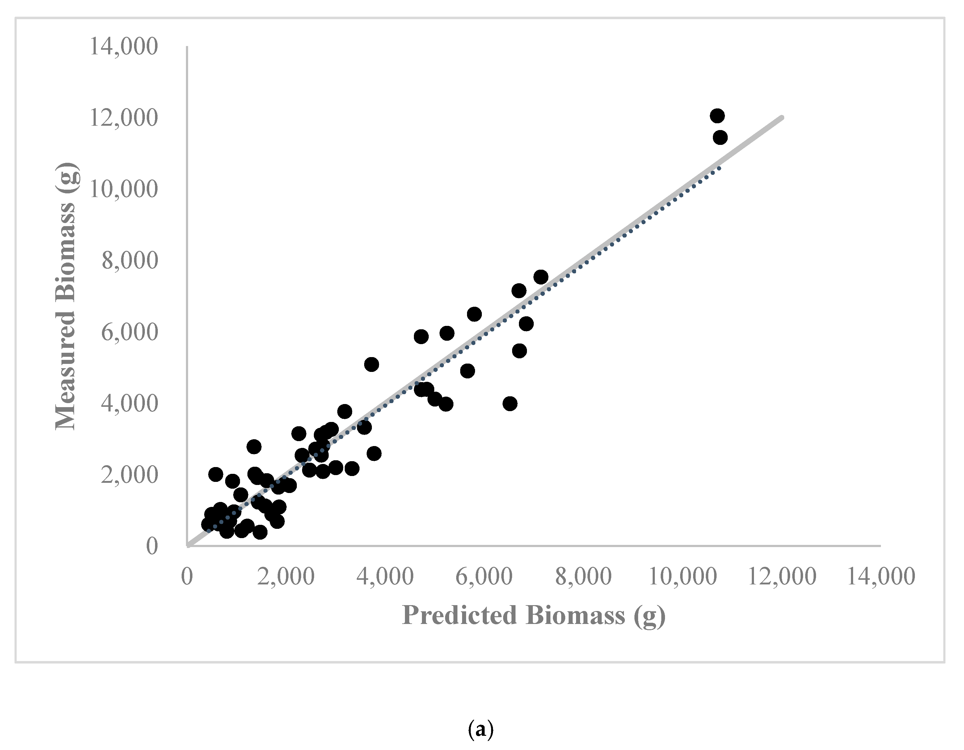
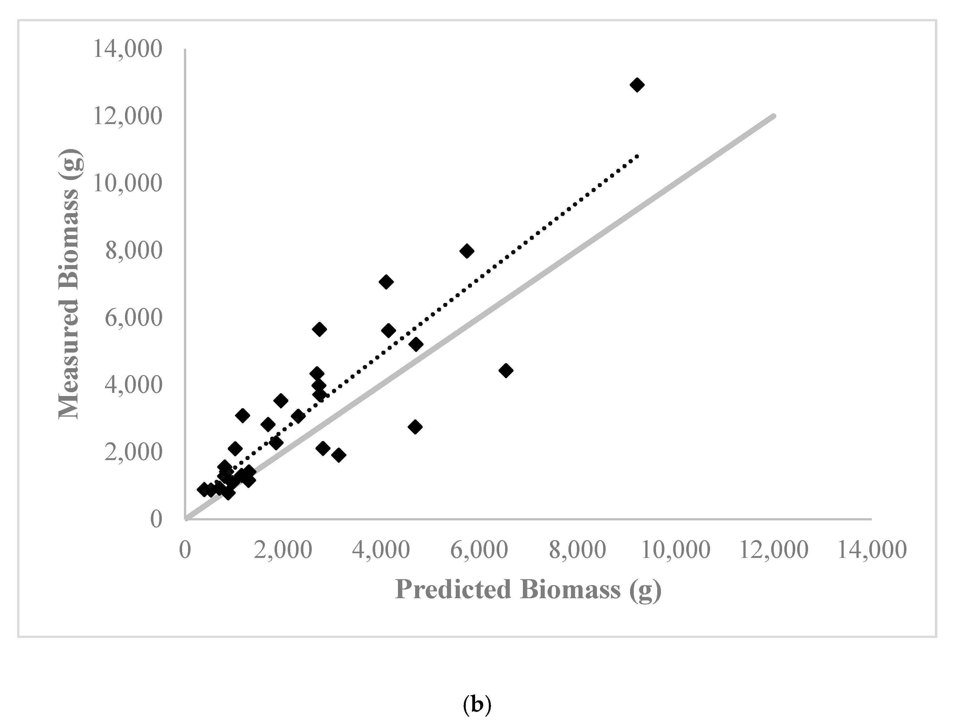
Table 5). Observed versus predicted values from each model showed a strong linear relationship at the calibration and validation sites; this relationship is visualized for one of the two top models (red ratio sum + MS red standard deviation) from the AIC model selection at both sites in
Appendix C (
Figure A1).
Validation site R
2 ranged from 0.732 for the CHM volume model to 0.773 for the model with three variables (
Table 5). Validation site RMSE as a percentage of mean total allometric AGB ranged from 44 to 100% and was highest for the green ratio sum + MS red max model and lowest for the NDRE model. Validation site MAE as a percentage of mean total allometric AGB ranged from 32% (NDRE model) to 86% (green ratio sum + MS red max model). Validation site MBE was always positive and was highest for the green ratio sum + MS red max model and lowest for the CHM volume model. The two models containing the NIR max variable had the lowest MBE, RMSE%, and MAE% out of the multivariate models.
3.5. Total Site-Wide Shrub Aboveground Biomass
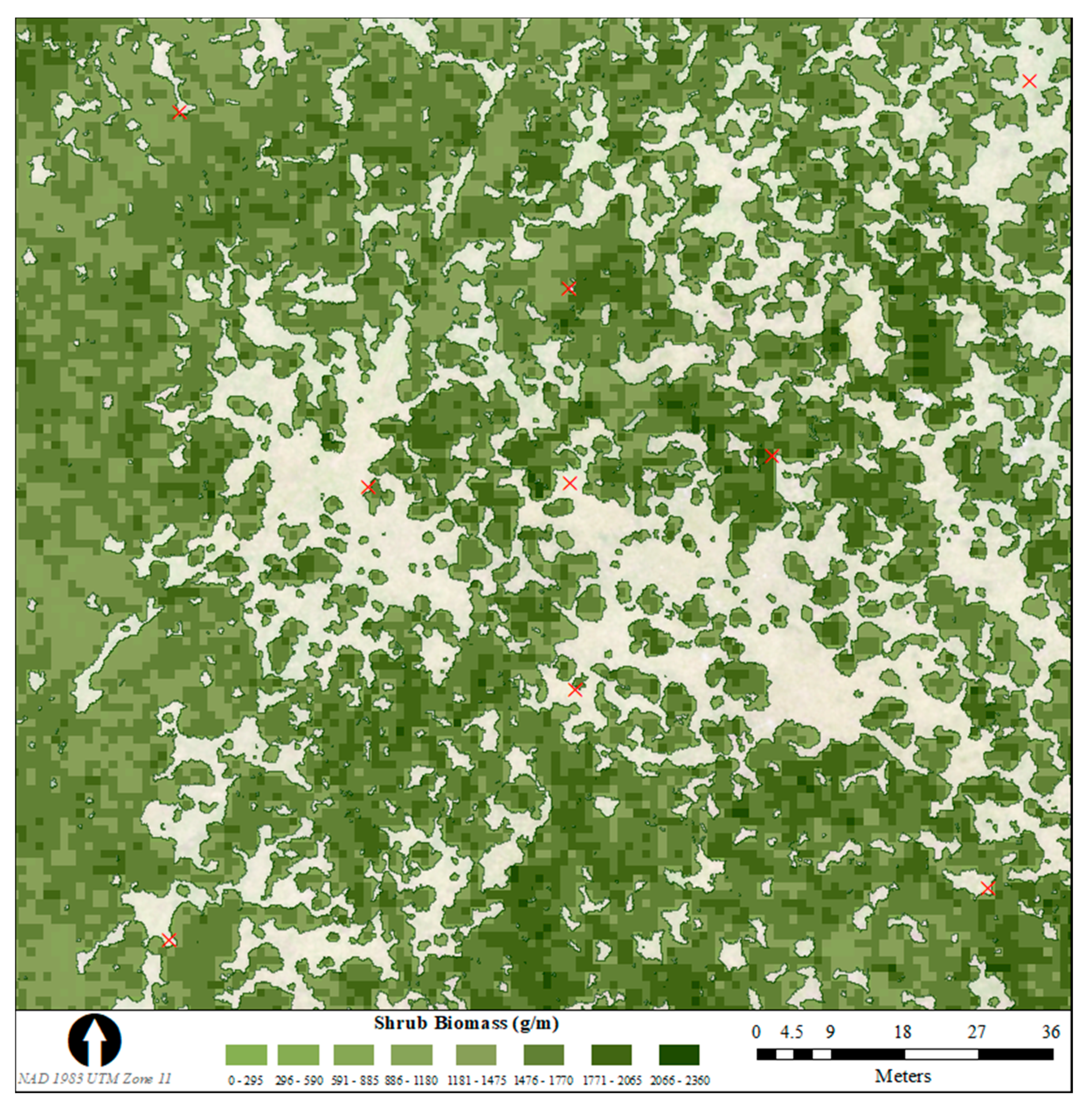
Using the classified shrub area, which covered 10,753 square metres of the study area, we extracted the total sum of values for the parameters from the top model as indicated by AIC model selection (red ratio sum + MS red standard deviation) and used the equation from the linear regression with allometric AGB to estimate total shrub AGB across the site. Total shrub AGB from the best model was 17,600 kgs, with an average of 1.64 kgs of shrub biomass per square metre of shrub-covered area and an average of 0.66 kgs/m
2 across the entire study area. The spatial distribution of shrub AGB across the study site is shown in
Figure 4.
4. Discussion
4.1. Accumulated Vegetation Index
Our analysis revealed that the aboveground biomass of shrubs in the
Betula and
Salix genera could accurately be modelled at a high spatial resolution using metrics derived from UAS imagery. The workflow developed in our study provides a way to estimate site-wide shrub AGB at a broader spatial scale than ground-based measurements and with a higher resolution than satellite imagery. We found that metrics using the sum of all VI values within each shrub outline, rather than measures of central tendency or deviation as are commonly used, had a superior performance over both CHM-based structural data and other spectral metrics. These “accumulated VIs” contain structural information about shrub canopy roughness and size in addition to spectral data [
61], capturing both spatial and spectral variations in shrub AGB within a single parsimonious metric. To our knowledge, other UAS-derived accumulated VI metrics for AGB estimation have not been described previously in the literature, although one study found that an RGB VI weighted by canopy volume was the best variable for estimating soybean crop AGB [
61].
In our study area dominated by shrubs with a low height (<2 m), the area-based VI accumulation approach was more useful for relating to shrub biomass than three-dimensional metrics such as height or volume, with accumulated VI metrics out-performing structural variables in single-variable models and showing a very strong linear relationship to ground-measured biomass. Shrub area alone (in metres squared) showed a high correlation (r = 0.88) and coefficient of determination (R2 = 0.824) with allometric shrub biomass, but the accumulated VI improved upon these values by including spectral as well as areal information. The accumulated VI appears to be ideal for AGB estimation for low-stature vegetation such as shrubs, fusing spectral and structural information into one metric with the advantage of not needing to create a CHM, which increases the amount of effort and uncertainty in biomass estimates. The low height of shrubs in our study area means that even small errors in a CHM could lead to biased estimates of shrub structure, affecting the ability of structural metrics to accurately predict biomass.
Model performance could be improved slightly over single-variable linear regressions by combining multiple uncorrelated metrics into one multiple regression model. For example, the two top models in the AIC selection contained two metrics—an accumulated ratio-based RGB VI and an MS metric using the red wavelength—and had the highest R
2 and lowest RMSE values of the tested models at the calibration site. Other UAS-based biomass studies also found that combining multiple data types into parametric or non-parametric regression models improved performance over single-variable models for various vegetation types [
28,
32,
44,
73]. Another found that shrub biomass could be modelled better by combining LiDAR-based height measurements with aerial imagery spectral data compared to LiDAR or aerial imagery alone [
22].
However, in our study the Δi value of <3 from the top model to the single variable accumulated red ratio model in the AIC model selection is only slightly over the AIC rule of thumb that models within two points of the best model have substantial support and a similar ability to explain variation in the data as the best model in the candidate set [
72]. This represents a marginal improvement in accuracy for the top model that requires deriving both MS and RGB variables, which increases effort of data collection by requiring multiple survey flights compared to the single-variable RGB VI sum models which are derived from a single RGB survey. Additionally, when applied to the validation site, the models with two or three predictor variables tended to have higher RMSE and/or MAE compared to the single-predictor variables, with the exception of models combining an RGB ratio-based sum metric with a NIR metric, which had a more stable performance in validation.
For the purposes of fine-scale site-wide shrub AGB estimation, we believe a parsimonious single-variable linear regression model containing the accumulated red ratio VI using data that can be collected from a single UAS survey is preferable over the slight increase in accuracy but concurrent increase in effort and uncertainty that would come from combining metrics from two different sensors for a multiple regression model. The accumulated VI metric provides a straightforward approach for shrub AGB estimation since data collection requires only a single UAS survey during peak vegetation greenness, which is ideal for streamlining workflows for management and monitoring of vegetation within a large national park such as Banff. We would be interested in investigating whether the sum of all VI values across the vegetated area relates similarly strongly to the biomass of other plant species or whether the biophysical characteristics of low-stature woody shrubs makes them the ideal vegetation type for this methodology.
4.2. Spectral Metric Comparison
RGB-based spectral metrics and VIs outperformed multispectral metrics for shrub biomass estimation in this study. Vegetation characterization with spectral information often uses non-visible wavelengths of electromagnetic radiation [
74], especially indices that use the near infrared or red edge region of the electromagnetic spectrum. However, despite being limited to visible wavelengths of light, RGB VIs can also be sensitive to biophysical characteristics of vegetation [
32,
75], and other researchers using UAS data to estimate vegetation biomass found that RGB VIs could outperform multispectral or hyperspectral VIs [
32,
36,
66,
76,
77]. Due to high correlations among the RGB and the MS variables, combining multiple RGB or multiple MS metrics in the same model did not improve model performance. Combining both RGB and MS metrics in the same model slightly increased accuracy over single-variable models, but this method requires conducting a survey with each sensor which increases data collection and processing effort.
Compared to the multispectral data, the smaller ground sampling distance of the RGB imagery collected in this study resulted in a higher spatial resolution (~1.5 cm pixels in RGB data, ~6 cm pixels in multispectral data). This means each individual shrub contained more pixels for use in analysis. The lower resolution of the multispectral imagery also meant that accurate classification of shrubs from these data is challenging, likely requiring the collection of RGB information to ensure accurate delineation of vegetation for applying site-wide biomass prediction models. Conducting a single UAS survey to collect RGB data that can be used for image classification and biomass estimation provides a logistically simpler process than collecting both types of imagery.
We found that the ratio-based RGB VIs were particularly useful for biomass estimation. Red ratio and green ratio both performed well in single-variable models, and both retained good performance when included in additive models an MS VI metric. This result was similar to another study using UAS data which found that the red ratio from RGB imagery was the best index for predicting winter wheat biomass among the RGB VIs tested [
66]. Ratio-based RGB VIs may be less sensitive to changes in illumination and atmospheric conditions over time compared to other VIs, making them more robust when conditions vary during data collection [
61].
Out of the multispectral bands and VIs tested, the model containing the NDRE variable performed the best for biomass prediction and had a more stable performance when applied at the validation site compared to the RGB VIs. This is likely because the multispectral data was radiometrically corrected. Red-edge indices have a strong relationship with leaf biomass and weaker relationship with stem biomass [
10,
23] and are sensitive to canopy structure [
70], making them useful for AGB estimation for vegetation species with large leaves or for growth stages of plants when the canopy is dominated by leaves. Red edge indices may also be slightly less prone to saturation than those using the NIR band [
18], and we found that NDRE outperformed the NIR band or NDVI alone. However, the two models that included a metric derived from the NIR band with a ratio-based RGB VI had lower MBE, MAE, and RMSE when applied to the validation site than other two-variable models. The NIR band may be useful in conjunction with RGB information for increasing the stability of models applied at other locations although including it in models with RGB VIs requires data collection with two different sensors.
4.3. Structural Metric Comparison
Out of the structural metrics tested, shrub volume demonstrated a greater ability than mean or maximum height to predict the aboveground biomass of individual shrubs, with coefficients of determination of ~0.75 with ground-based biomass in calibration models and ~0.73 in validation, although these values were lower than those of the RGB and multispectral models. Canopy volume calculated from UAS imagery was found to have a good ability to predict aboveground biomass of Arctic shrubs [
9], as well as of other vegetation including boreal forest trees [
31], onion plants [
39], and soybean crops [
61]. Compared to height metrics alone, volume metrics capture variation in vegetation height and density simultaneously [
39], characterizing canopy structure traits in both vertical and horizontal dimensions [
61].
We found similar or higher accuracy in the ability to model shrub AGB from volume compared to height, as did studies using LiDAR-based height metrics [
10,
21,
78,
79]. Conversely, studies using shrub volume derived from terrestrial laser scanning found stronger positive relationships to aboveground shrub biomass, with R
2 values >0.85 [
16,
80,
81], demonstrating that volume metrics may relate more strongly to shrub biomass than height metrics alone [
10,
21,
22,
78]. UAS-derived point clouds usually have a very high point density closer to terrestrial than to aerial laser scanning, but laser scanning has a greater ability to penetrate through vegetation to the terrain, which may explain why terrestrial laser scanning-based shrub biomass estimates using volume had higher coefficients of determination than those found in this study.
There is likely to be greater uncertainty and more error in vegetation volume estimates from UAS CHM models compared to terrestrial laser scanning due to the difficulty of accurately characterizing the terrain beneath dense vegetation in UAS imagery. Over- or underestimation of local terrain variations and misclassification of terrain as vegetation or vice versa can lead to biased estimates of structural metrics and biomass compared to field measurements [
31]. Several studies using UAS data to estimate deciduous and coniferous tree biomass found that tree height from a CHM was underestimated compared to field measurements [
41,
43,
62,
63]. We found that shrub biomass was approximately equally over- and underestimated by CHM volume, although the biomass of smaller shrubs was more often overestimated and larger shrubs more often underestimated, a pattern found by other UAS-based vegetation biomass studies [
44,
73,
75,
82].
4.4. Site-Wide Aboveground Biomass
An important finding in this study was the linear relationship between our predictor variables and shrub AGB, which means that classification of shrubs in order to apply the AGB prediction equation is not necessary to the individual plant level, even though our equations were derived for individual plants. Rather, the area covered by shrubs is all that is needed, over which the total sum of RGB VI values can be calculated and used in the equation to linearly predict total shrub AGB across the shrub class. This result is similar to that found by the existing published study using UAS data to estimate shrub AGB [
9] as well as to studies using terrestrial LiDAR to quantify aboveground biomass of sagebrush shrubs [
10], which also reported a linear relationship between shrub AGB and shrub area. This methodology produces straightforward results that are easy to apply and interpret compared to more complex procedures that require identification of individual plants.
By applying the parameter estimates derived from our best models across the entire ~10,800 square metre region covered by shrubs within our study site, we calculated approximately 17,600 kg of total shrub aboveground biomass, corresponding to an average of 1.64 kgs/m
2 in the area covered by shrubs. This is comparable to the results of Cunliffe et al. [
9] who used shrub volume calculated from a UAS-derived CHM to estimate AGB of creosotebush and juniper shrubs in a dryland ecosystem, finding an average AGB of 1.45 kg/m
3 and 2.55 kg/m
3 for each species respectively. Across the entire study area the average of 0.66 kg/m
2 was similar to the 0.65 kgs/m
2 reported in shrubland environments in the adjacent foothills region of the central east slopes of the Rocky Mountains [
83].
When estimating the carrying capacity of bison within the reintroduction zone in Banff National Park, Steenweg et al. [
54] calculated a total winter shrub intake rate of bison to be ~97 kg over 181 days of winter. With 35 bison reported in the Banff herd as of winter 2019, if all animals stayed within our study site for the winter, they would consume approximately 3492 kgs of shrub AGB, just over one tenth of what is available within the site. Our study area represents a very small fraction of the total bison reintroduction zone, so there is far more than the minimum shrub forage requirements calculated for the herd. Since other ungulates such as elk are also likely to browse on shrubs within the bison reintroduction zone [
84], estimates of shrub AGB within Banff National Park are useful for understanding the availability of potential ungulate forage at a given point in time.
4.5. Browsing Detection
To determine if the high resolution of UAS imagery allowed changes in shrub AGB due to browsing to be detected using multi-temporal data, we conducted one UAS flight at the calibration site immediately after we manually “browsed” the 60 sample shrubs by using clippers to remove the leaves and twig ends in a manner similar to a browsing ungulate. We created a CHM, using the browsed shrub DSM, and calculated RGB VIs from the browsed model in the same way as with the non-browsed model, then identified and manually outlined an additional 60 shrubs that were clearly visible in the imagery and were not browsed. We then compared the change in CHM and RGB VI values between the browsed and un-browsed shrubs from before and after browsing to determine if a change could be detected.
Without radiometric correction, changes in reflectance values of RGB VIs across all shrubs due to very different illumination conditions for each survey flight were stronger than any signal that the browsing may have given and so were unable to detect changes in RGB VIs due to browsing. It would be valuable to determine if radiometric normalization of the imagery taken on different dates would make multi-temporal data more comparable and allow detection of changes in spectral values on the browsed shrubs caused by decreases in biomass due to removal of leaves and twigs via browsing.
Conversely, we were able to detect a change in shrub volume from the CHM in the browsed versus un-browsed shrubs. Un-browsed shrubs showed a mean change in volume of around 11% between the two data collection dates, which is within the range we would expect volume to change due to shrub movement in the wind and slight variations in illumination between image collection dates. Browsed shrubs decreased in volume by an average of 75%, much more than would be expected due to shrub movement, indicating that changes in shrub AGB due to browsing by wildlife could be detected in UAS imagery. This approach may be useful for wildlife research and management where there is an interest in understanding fine-scale forage consumption and changes in forage availability over time.
4.6. Allometric Equations
We used a general shrub allometric equation developed previously in our study area [
57] to calculate ground-based shrub AGB, making the assumption that relationships between shrub basal stem diameter and biomass had remained constant over the 12 years between the development and our application of the allometric equation. The application of generalized rather than species-specific allometric equations is not uncommon, especially for site-wide biomass estimates or in mixed-species environments when developing individual equations would be impractical [
85]. For example, previous research in Alberta found no significant difference in the performance of species-specific and general shrub allometric equations for three shrub species in a boreal peatland [
86].
In our study area,
Betula and
Salix shrubs have similar ranges of shapes and sizes, making a general shrub equation suitable for AGB estimation. However, when shrub species show greater variation in stem size and biomass, species- or genus-specific equations developed for that site are likely to have a stronger performance than general equations [
87]. Additionally, applying general allometric equations to a new region, a species not included in the development of the equation, or to shrubs that fall outside of the domain of sizes over which that equation was developed can have lower accuracy and requires validation [
86,
88]. If possible, we recommend that researchers conduct destructive sampling of shrubs at their study site to validate existing allometric equations or derive new ones if there is an interest in highly-accurate biomass measurements, especially at the scale of individual shrubs [
85,
88].
4.7. Limitations and Recommendations
Despite their good performance in this study, there are constraints to UAS-derived RGB VIs that researchers should consider when using them to estimate vegetation AGB. Automatic or pre-set exposure settings on many RGB cameras are based on overall light intensity, which can vary between images due to changes in solar elevation and clouds [
77,
89,
90], and small changes in radiation may lead to large differences in image tone unrelated to actual properties of the vegetation [
36]. Extrapolating results from RGB data that has not been radiometrically corrected should be done with caution. Researchers should plan data collection and analysis to include radiometric correction methods, such as an empirical line calibration, which was originally developed for satellite imagery but can also be used for radiometric normalization of RGB and multispectral imagery [
34,
91,
92].
In this study we could apply non-radiometrically corrected RGB VI-based models to predict shrub AGB at the validation site and still achieve strong model performance (R2 > 0.75). However, the RMSE and MAE of the RGB models were much higher than that of the multispectral or CHM volume models when applied to the validation site, reaching up to 100% of observed AGB values. Similarly, the MBE indicated much greater overestimation of shrub AGB from the multivariate or RGB VI models compared to CHM volume or NDRE models or the two models that combined ratio-based RGB VIs with a NIR metric. This overestimation in the RGB models likely occurred because while the multispectral sensor comes with a radiometric target to calibrate reflectance values in the imagery and the CHM volume is less influenced by radiometric differences between sites, the RGB data were radiometrically uncorrected and so had a wider margin of error when models developed at one site were applied to another. However, the strong linear relationship between predicted and observed biomass values was still present in RGB VI models at the validation site. We expect that if data collection and analysis was planned to include radiometric correction of RGB imagery, the ability of models derived from these data to predict shrub biomass would be stronger with less error and bias in biomass estimates, allowing researchers to develop biomass prediction models at one site and apply them with confidence to other sites without the need for conducting multiple surveys with different sensors.
Although the volume structural metric did not relate as strongly to measured shrub biomass as spectral metrics, the single-variable regression model containing volume had a stable performance when applied at the validation site, with very similar R
2 values between the two sites and relatively low RMSE, MAE, and MBE in validation, indicating less variation and bias in predicted biomass values when applied to a new spatial location compared to the non-radiometrically corrected VI-based models. The CHM was also useful for distinguishing shrub and non-shrub areas of the site during image classification, and changes in shrub AGB due to browsing were more detectable in the CHM volume than using spectral information. It is possible that difficulties interpolating the terrain beneath the shrub canopy when creating a DTM influenced the performance of our CHM as dense vegetation is known to make interpolation of an accurate terrain model from UAS imagery challenging [
2,
41,
43,
48]. Although the accumulated VI metrics were able to accurately estimate shrub AGB, it may be worth further exploring whether DTM creation and CHM-derived volume measurements can be improved for prediction of shrub AGB.
Single-variable linear regressions had equal or higher accuracy to multiple regression models combining several predictor variables. As an alternative to linear regression models, we could have combined all our spectral and structural predictors into machine learning regression algorithms. Machine learning regressions are being increasingly used with remotely-sensed data due to their ability to handle a high number of inter-correlated predictor variables that may have a non-linear relationship with the dependent variable [
34,
38,
73,
76]. Some researchers comparing machine learning random forest (RF) models with alternate model forms for vegetation biomass estimation from UAS data found that RF models equaled or outperformed parametric regressions [
34,
66,
73].
However, non-parametric regression methods are more complex to implement and interpret as they do not express relationships between the predictor and dependent variables in a single equation, losing some of the biological and physical meaning of a simple regression. Other researchers found that UAS data could predict vegetation AGB with equal or higher accuracy from simple regressions compared to machine learning methods [
5,
61,
73]. For the purposes of broad-scale vegetation monitoring, linear regression models represent a straightforward and biologically-understandable approach to AGB modelling, and given the strong performance of the simple regressions relating RGB VI sum metrics to biomass found in this study, we believe that a potential increase in model accuracy from a machine-learning regression is not worth the increased computational effort and more opaque model application of this approach.
Finally, we note the reliance on allometric equations to derive our AGB reference data, a concession required by the remote helicopter-access location of our field sites. We advise future researchers to validate our findings with direct AGB measurements.


