Abstract
Remote sensing images classification is the key technology for monitoring forest changes. Texture features have been demonstrated to have better effectiveness than spectral features in the improvement of the classification accuracy. The accuracy of extracting texture information by window-based method depends on the choice of the window size. Moreover, the size should ideally match the spatial scale of the object or class under consideration. However, most of the existing texture feature extraction methods are all based on a single window and do not adequately consider the scale of different objects. Our first proposition is to use a composite window for extracting texture features, which is a small window surrounded by a larger window. Our second proposition is to reinforce the performance of the trained ensemble classifier by training it using only the most important features. Considering the advantages of random forest classifier, such as fast training speed and few parameters, these features feed this classifier. Measures of feature importance are estimated along with the growth of the base classifiers, here decision trees. We aim to classify each pixel of the forest images disturbed by hurricanes and fires in three classes, damaged, not damaged, or unknown, as this could be used to compute time-dependent aggregates. In this study, two research areas—Nezer Forest in France and Blue Mountain Forest in Australia—are utilized to validating the effectiveness of the proposed method. Numerical simulations show increased performance and improved monitoring ability of forest disturbance when using these two propositions. When compared with the reference methods, the best increase of the overall accuracy obtained by the proposed algorithm is 4.77% and 2.96% on the Nezer forest data and Blue Mountain forest data, respectively.
1. Introduction
As an integral part of natural ecosystems, forests not only regulate the circulation of air and water in nature and protect the soil from wind and rain, they also reduce the harm caused by environmental pollution to people. The complete or partial destruction of forest and vegetation cover generally results in many adverse consequences in the ecosystem, including an intensification of runoff and erosive processes, loss of biodiversity, and impact on global warming [1].
In recent years, climate change has made extreme weather more and more frequent. Hurricanes and fires are two types of natural disturbances to forest ecosystems [2,3]. A severe hurricane can widely impact on the vegetation composition, structure, and succession of forests, and accordingly influence the terrestrial carbon sink [4,5]. Damages from fires, a common and prevalent disturbance that affects the forest [3,6,7,8], can be severe, reducing species richness and above-ground live biomass [9]. Between 2015 and 2020, ~10 m hectares of the world’s forests have been lost each year according to the records of the Food and Agriculture Organization of the United Nations [10].
It is of great significance to map the windfall damages of forests and estimate the affected areas for the post-disaster management [11]. However, field-based studies are time-consuming, laborious, and usually only cover small areas, in consideration of the time and cost, of making the observations. Moreover, forest disasters generally happen in remote regions [12], and as such can be hard to reach for in situ measurements [13]. Consequently, using these methods is constrained to an extremely limited spatial and temporal extent. On the contrary, as exemplified in [14,15,16,17], remote sensing offers an opportunity to accurately assess all areas covered by damages in a reliable, cost-effective, and time-efficient manner, to the extent that machine learning provides accurate classifying tools.
A substantial number of approaches have been devised for monitoring forest changes using remote sensing images classification [18,19]. For example, Zarco-Tejada et al. detected forest decline using high-resolution hyperspectral and Sentinel-2a imagery [20]. White et al. evaluated the utility of a spectral index of recovery based on the Normalized Burn Ratio (NBR): the years to recovery, as an indicator of the return of forest vegetation following forest harvest (clear-cutting) [21]. Bar et al. identified pre-monsoonal forest fire patches over Uttarakhand Himalaya using medium resolution optical satellite data [22]. However, most of these methods pay more attention to only utilize the spectral features derived from image pixels. The feature limitation could not solve the problem of similar reflectance characteristics coming from different objects, thus leads to a decrease in classification accuracy.
In later research endeavors, apart from the spectral information, texture features have been widely used in image classification to assist in the discrimination of different target classes with similar spectral features [23,24]. They provide an opportunity to increase the classification performance of the forest disturbances, specifically for forest hurricane and forest fire disturbance mapping. For example, Jiang et al. computed texture features of the image to recognize forest fire smog [25]. The recognition accuracy is 98% with robustness on their smog image database. Benjamin et al. extracted the fire region from forest fire images using color rules and texture analysis [26]. Kulkarni et al. used the local fractal TPSA method to compute the textural features of the image and evaluated the impacts of Hurricane Hugo on the land cover of Francis Marion National Forest, South Carolina [27]. Textural features are statistical measures of the spatial arrangement of the gray-level intensities of an image [28,29]. Generally, texture feature extraction approaches are applied to pixels of the input image by evaluating some type of difference among neighboring pixels through square windows that overlap over the entire image [30]. The accuracy of extracting texture information by window-based method depends on the choice of various parameters. For example, the study by Marceau et al. [31] proved that the window size is the most crucial parameter impacting classification accuracy. Murray et al. systematically analyzed the influence of the window size and texture feature selection on classification accuracy [32]. Garcia et al. analyzed the part played by both the shape and size of the window, then indicated that texture features are much more affected by the window size than by its shape [33].
In fact, the size of the texture window should ideally match the spatial scale of the object or class under consideration. However, the aforementioned texture feature extraction methods are all based on a single window. In other words, the single window approaches do not adequately consider the scale of different objects, and always face the trade-off problem between window size and classification accuracy [32]. On the one hand, the window size should be large enough to obtain the relevant patterns, but if the size is too large, edge effects could dominate the results [34]. On the other hand, finding precise localizations of boundary edges between adjacent regions is a fundamental goal for the segmentation task, but it can only be ensured with relatively small windows [30]. Consequently, how to obtain a good texture characterization is a very important research direction for the improvement of the image classification accuracy.
Ensemble learning techniques have been successfully applied to remote sensing image classification and are attracting more attention for their increased performance in accuracy [35,36,37,38,39,40]. They carry out various training tasks inducing multiple base classifiers whose outcomes are fused into a final prediction. Random Forest (RF) is a very powerful ensemble algorithm. It is a collection of decision trees usually induced with the Classification and Regression Trees algorithm (CART) [41]. RF has been widely used for forest disturbance mapping. For example, Einzmann et al. used the RF classifier to detect the area damaged by the hurricane [42]. Their methodology was evaluated on two test sites in Bavaria with RapidEye data at 5 m pixel resolution and identified over 90% of the windthrow areas. Ramo et al. developed an RF algorithm for MODIS global burned area classification [43]. To assess the performance of their methods, these models are used to classify daily MCD43A4 images in three test sites for three consecutive years (2006–2008). Considering the advantages of random forest, such as fast training speed and few parameters, random forest is also used for forest disaster monitoring in this paper. In the application under focus, we assume that a fair amount of already classified pixels are available for training. These pixels should be relevant by having sufficiently similar reflectance characteristics, and yet in general, they should not be expected, to be part of the studied image. In RF, base classifiers are decision trees, and diversity is achieved by multiple random samplings of both the training set and the feature set. Outcomes of all decision trees are combined based upon majority rule. As a supplementary benefit and with no extra computations, the training of decision trees provides measurements of feature importance. These measurements are used for feature selection, as a dimension reduction technique improving the ability to discriminate between classes.
Our aim is to classify pixels from a multispectral image captured over a forest landscape, into three classes—damaged, not damaged, and unknown—denoted here as , , and , respectively. The specific objectives of this study are to (1) develop a new algorithm for extracting texture features, more specifically, using a composite window; (2) utilize the importance of features calculated while using RF for feature selection as a class-discriminative dimension reduction tool; and (3) validate this algorithm. Finally, the texture features extracted from this study could improve the classification accuracy of remote sensing images and enhance the monitoring ability of forest disturbance.
The structure of this paper is as follows. Section 2 of this paper describes the studied area and the imagery being used for this study. In Section 3, the proposed method is presented. Section 4 presents the results and the analysis, including the overall accuracy, the kappa coefficient, the per-class accuracy, the per-class area, and color maps towards evaluating forest damage. The discussion is presented in Section 5. Section 6 shows the conclusions that can be drawn from the methods and results.
2. Material
2.1. Study Area
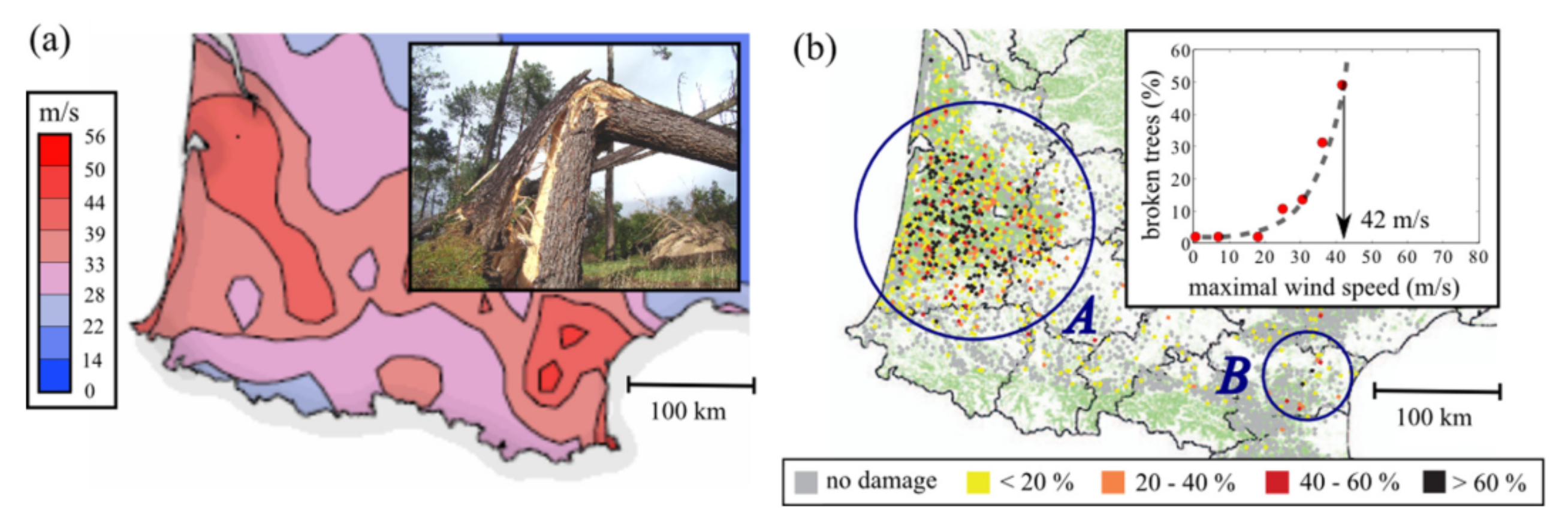
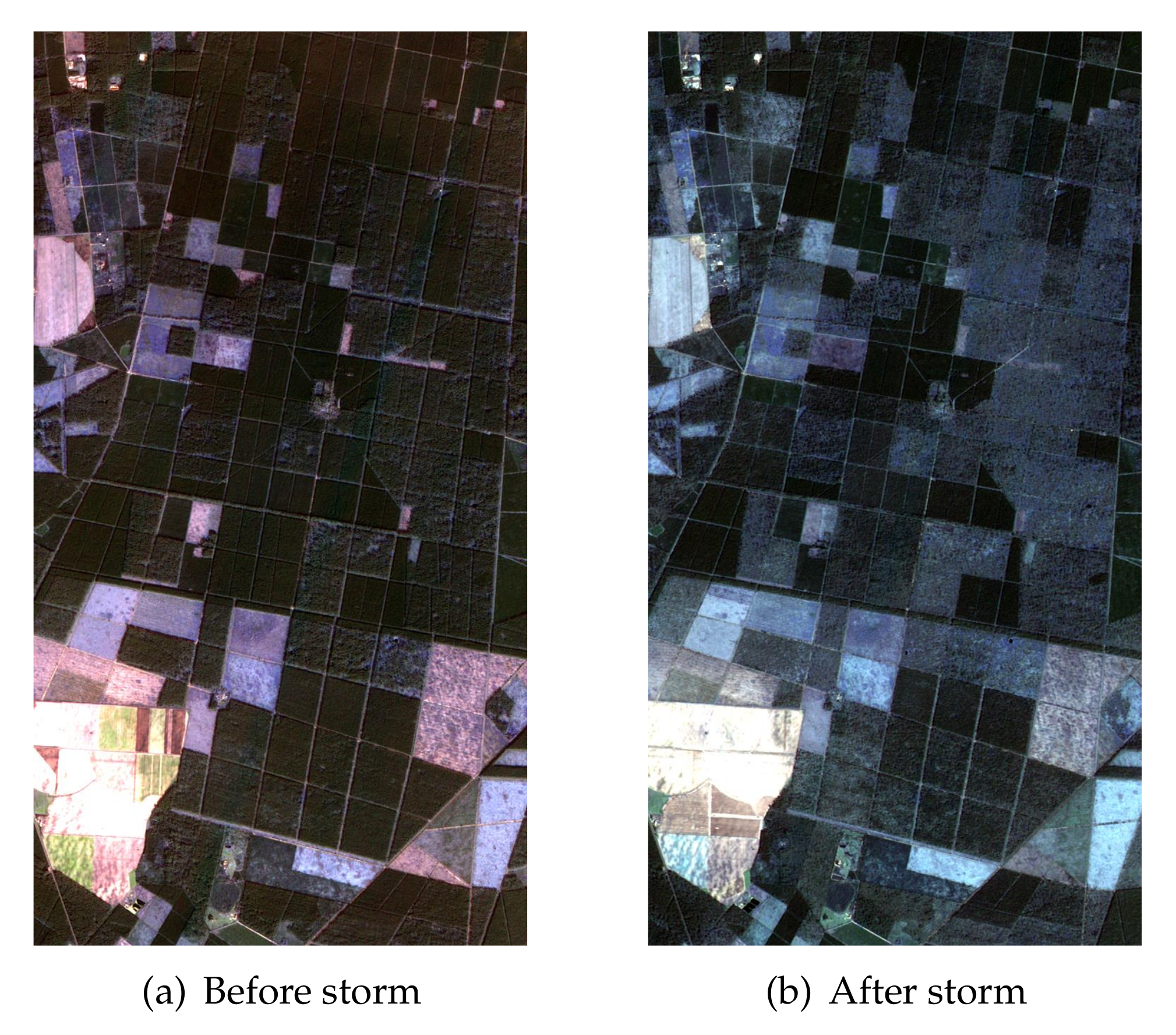
Nezer forest and Blue Mountain forest are the two studied areas shown in Figure 1. Nezer forest covers approximately 60 km and is located near the Atlantic coast in southwest France, within a large European maritime pine forest. Figure 2 presents maximal wind speed recorded during the storm Klaus and the damage to trees in France [44]. As we can see from Figure 2b, the southwestern part of France, where we studied, was severely damaged by the storm. Figure 3 shows the bitemporal Formosat-2 image from pre- and post-Windstorm Klaus, acquired on 22 December 2008 and 4 February 2009, respectively. Only the second image is being used here. The images have 8 m spatial resolution and four spectral bands (red, green, blue, and near-infrared). Image radiance is rescaled between 0 and 255. We performed atmospheric correction on this data through ENVI (5.3). The atmospheric model is Sub-Arctic Winter and the aerosol model is rural. Besides, the aerosol retrieval we selected is 2-band (K-T). The other parameters were set by default. All images are orthorectified and georeferenced. We have been provided with an already labeled classification of the second image in the three classes (, , and ). This is based on an exhaustive visual inspection by comparing Figure 3a,b, and recorded on a georeferenced map of locations of damaged and undamaged areas.
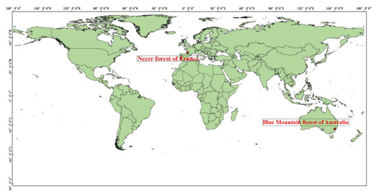
Figure 1.
The locations of two study areas.
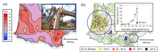
Figure 2.
Storm Klaus (Southwest France, 24 January 2009). (a) Maximal wind speed recorded during the storm Klaus (Data: Meteo France [45]). (b) Percentage of broken trees attributed to the storm Klaus. (Data: Inventaire Forestier National [46]).

Figure 3.
Formosat-2 multispectral images acquired before and after Windstorm Klaus.
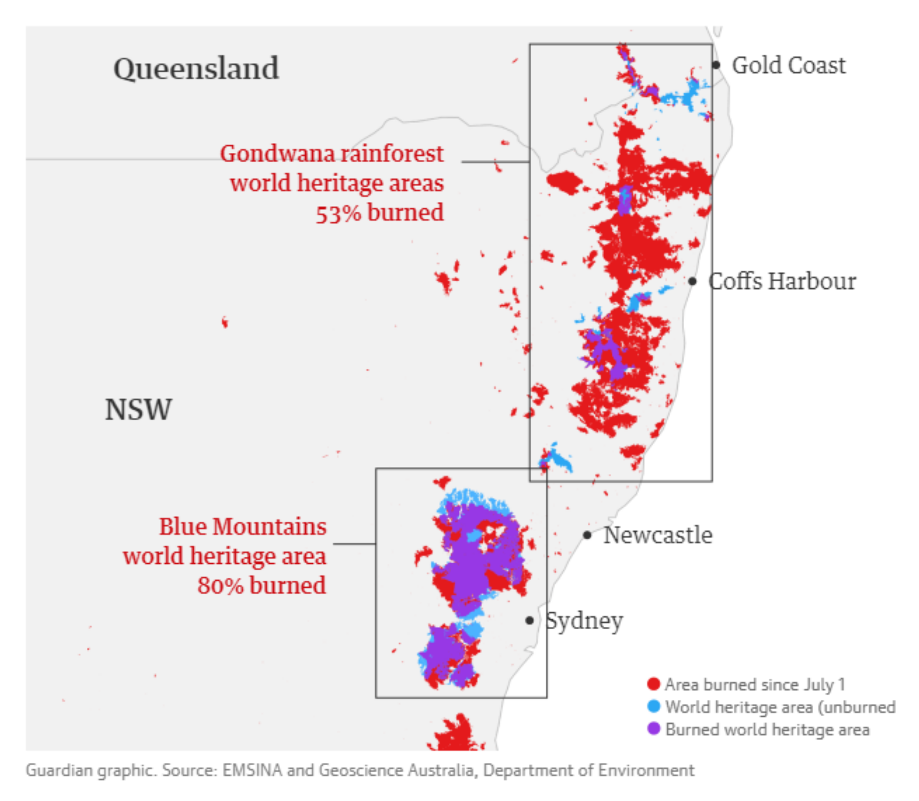
The second studied area is located in the southwest of the Blue Mountains National Park, which is located in the territory of New South Wales, approximately 100 km from Sydney, Australia. Covering an area of approximately square kilometers, Blue Mountain forest is home to large areas of virgin forest and subtropical rain forest, of which the eucalyptus tree is the most famous, the national tree of Australia. Figure 4, which is provided by EMSINA and Geoscience Australia, Department of Environment, presents where fire agency maps of burned areas and world heritage areas overlap [47]. Eighty percent of Blue Mountains rainforests in which our study area is located were burnt in bush fires. Figure 5 shows the two satellite remote sensing images (before and after the fire) obtained through sentinel-2A in 22 October 2019 and 31 December 2019. Only the second image is being used here. The remote-sensing images are orthogonally corrected and geometrically corrected, with a resolution of 10 m and 13 bands. Utilizing a similar exhaustive visual inspection, we have been provided with an already labeled classification of the second image in the same three classes ().

Figure 4.
Fire agency maps of burned areas and world heritage areas overlap [47].
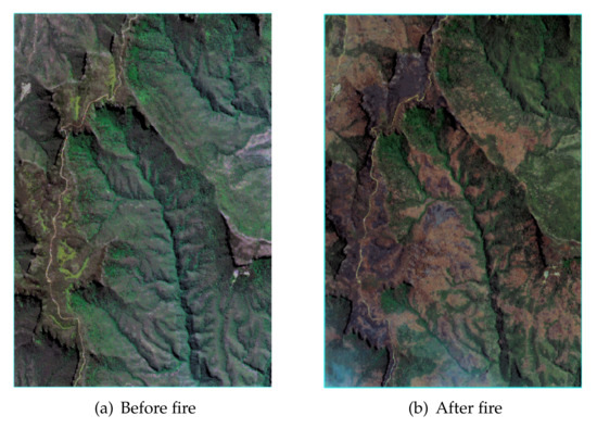
Figure 5.
Sentinel-2A multispectral images acquired before and after Fire Austrilia.
2.2. The Sample Data
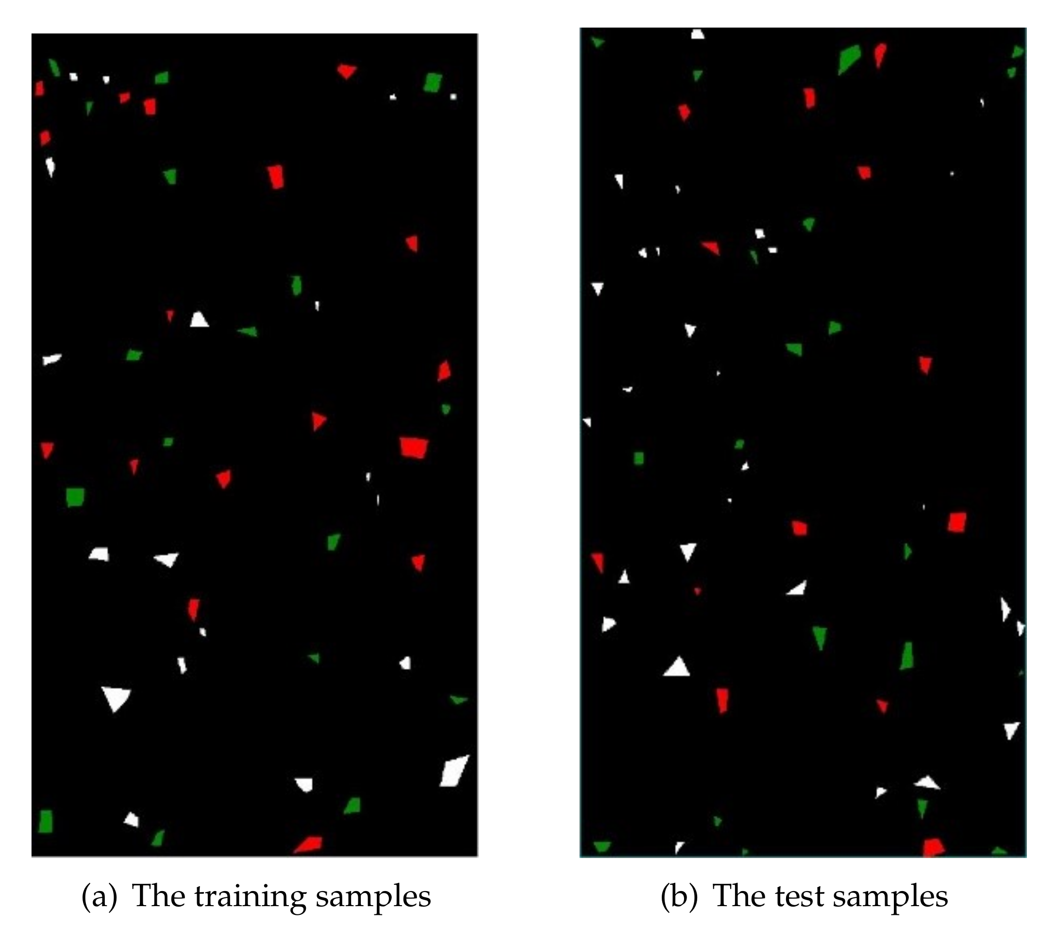
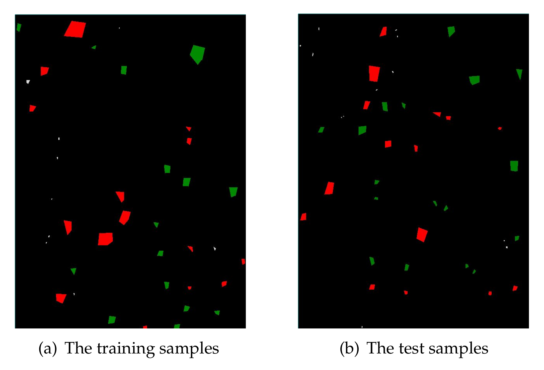
Samples have been evenly and randomly split into the training set and the test set , regardless of their class membership. For Nezer Forest, the training and the test samples were shown in Figure 6a and Figure 6b, respectively. For Blue Mountain Forest, the training and the test samples were exhibited in Figure 7a and Figure 7b, respectively. We note that the training set and the test set for both research areas are all independent. In two figures, red, green, and white represent the damaged, undamaged, and unknown object, respectively.
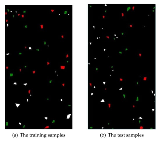
Figure 6.
Training and test samples of Nezer Forest data.
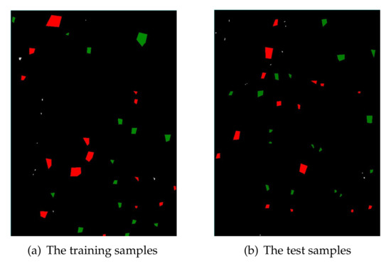
Figure 7.
Training and test samples of Blue Mountain Forest data.
Table 1 and Table 2, respectively, display the amount of training and testing samples from each of the three classes () for both images (Nezer Forest and Blue Mountain Forest). Interestingly, both datasets are fairly balanced between the and classes. Note that when comparing the training set and the testing set, it appears that the two-class distributions are different. This is caused by the randomization and it has been left unchanged, as such may occur in the application considered.

Table 1.
Training and testing samples of the Nezer Forest.

Table 2.
Training and testing samples of the Blue Mountain Forest.
3. The Proposed Method
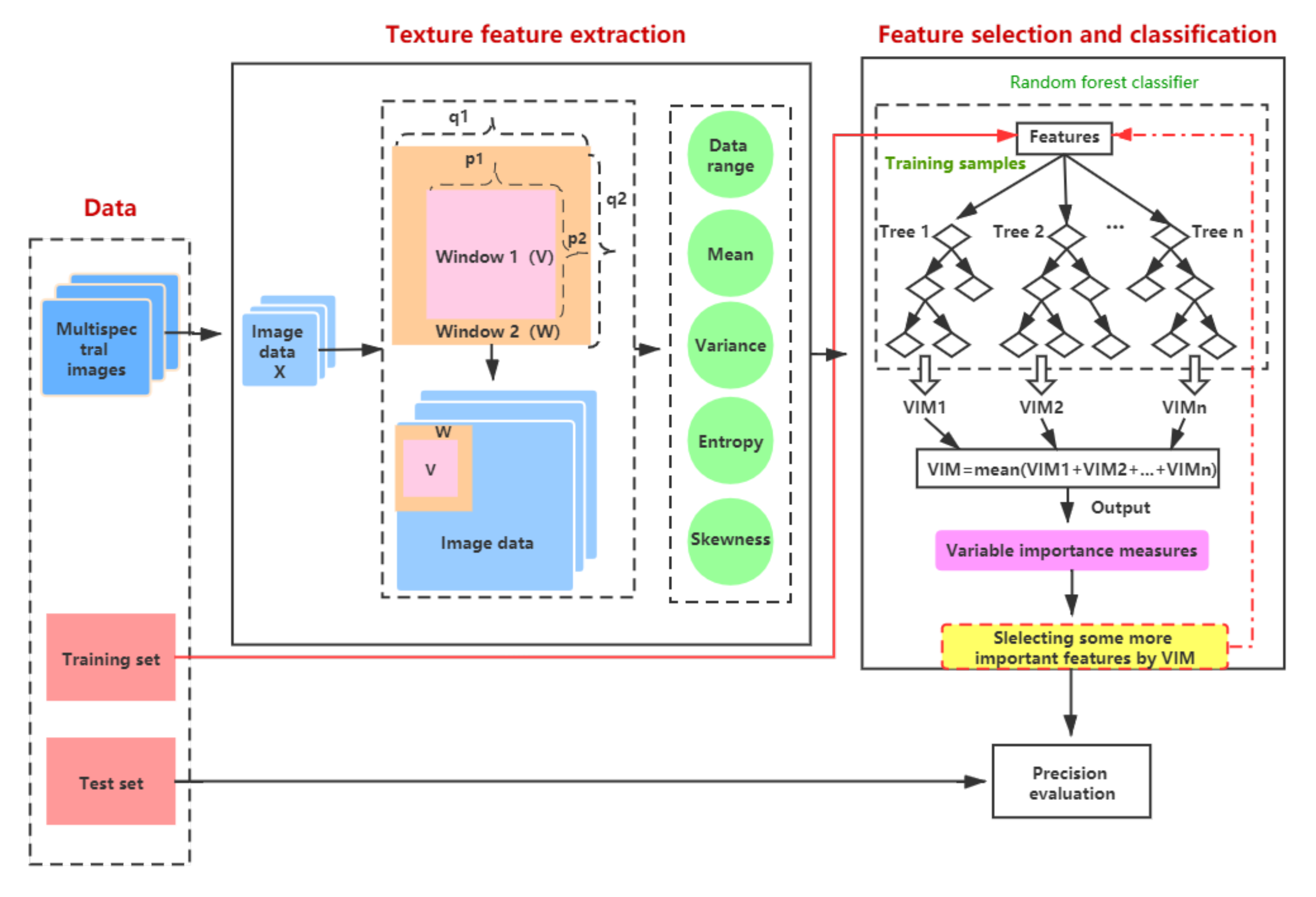
The proposed training method is summarized in a flowchart shown in Figure 8. On the left of the flowchart, a multispectral image is depicted as a stack of images (i.e., one image for each wavelength). The “preprocessing” indicated with a right arrow is here represented by normalization mapping pixel values in the range of . At the upper center of the flowchart, there is a large frame entitled “Texture feature extraction” transforming images into feature values. Pixels inside windows have specific spatial coordinates assembled in two sets: for the smaller window and for the larger one. These images are first scanned by a composite window as disclosed in Section 3.1. From pixels inside each window, five feature values are then extracted, as enumerated in Section 3.2. On the right of the flowchart, there is a frame entitled “Feature selection and classification” which figures two tasks. The extracted feature values feed an RF ensemble classifier, as summarized in Section 3.3. Besides, while the base classifiers are being trained, measurements of feature importance are first readout, then used for feature selection, as explained in Section 3.4. The proposed training method is sketched in Algorithm. The actual feature values used to train the ensemble classifier, come from the training set. Moreover, labels of the test set are compared to predictions of the trained ensemble classifier. Those connections are indicated with two long arrows at the bottom of the flowchart and the comparisons of these predictions are figured with a small frame entitled “Prediction evaluation” at the bottom right of the flowchart. Equations of these comparisons are given in Section 3.5. The parameter setting will be presented in Section 3.6.
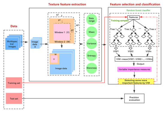
Figure 8.
Technical flowchart.
3.1. Scanning with a Composite Window
The composite window proposed here is a set of two windows sharing the same center, the first being larger than the second one. To ease notations, windows are assumed to be square and their sizes to be odd integers. Their respective sizes can be written as and . With a size denoted as , multispectral images are processed in a raster scanning order with a stride of 1. There are possible locations for both windows as they are moved together ( is a set containing all possible k-indexes). Some locations are discarded when they would be centers of windows exceeding the image’s size.
The coordinates of their common center is
where .
Values extracted from both windows are
where is the pixel value at location and wavelength is indexed by d.
This composite windowing technique is illustrated on the left of Figure 9 showing a flowchart of the feature extraction process with values specific to the Nezer dataset. The four superimposed darker squares are figuring a multispectral image with four wavelengths, and from which can be extracted four specific images, denoted in equations as . On the upper left corner of the first frame, a white square contains inside itself a gray square. Both squares are figuring the first location of the two windows sharing a common center as indicated by a left-oriented arrow. The central part of the Nezer-specific flowchart lists eight windows; there are two windows for each captured wavelength. These windows are specific to each location, so from a multispectral image, there are windows.
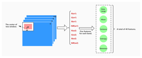
Figure 9.
The feature extraction procedure.
Note an unusual consequence of this windowing process in terms of machine learning, because features are actually extracted from pixels inside moving windows, the real training and test set should not be considered each as a set of pixels, rather as sets of pixels contained in windows, whose centers are, respectively, in the so-called training and test sets. Some training and test sets may have common pixels. While the reader ought to bear in mind this puzzling oddity, we think that this is not too much an issue, as this experimental setting is used here for comparison purposes. For the sake of simplicity, the training and test sets mentioned in the following sections are described as featured pixels, not sets of pixels.
3.2. Texture Features Extracted
The flowchart of Figure 9 shows on its right a list of five features (Data range, Mean, Variance, Entropy, and Skewness), extracted from each of the windows available at each k-indexed location. These features are defined in the following equations, all computed using only values of pixels inside a given window. They are denoted as when extracted from the smaller window, and when extracted from the larger window, r being a feature-index ranging from 1 to 5.
- and are data ranges and defined as the difference between the maximum pixel value and the pixel minimum value.
- and are means computed by adding all pixel values and dividing by their number.
- and are variances computed by averaging the square differences between pixel values and their means.
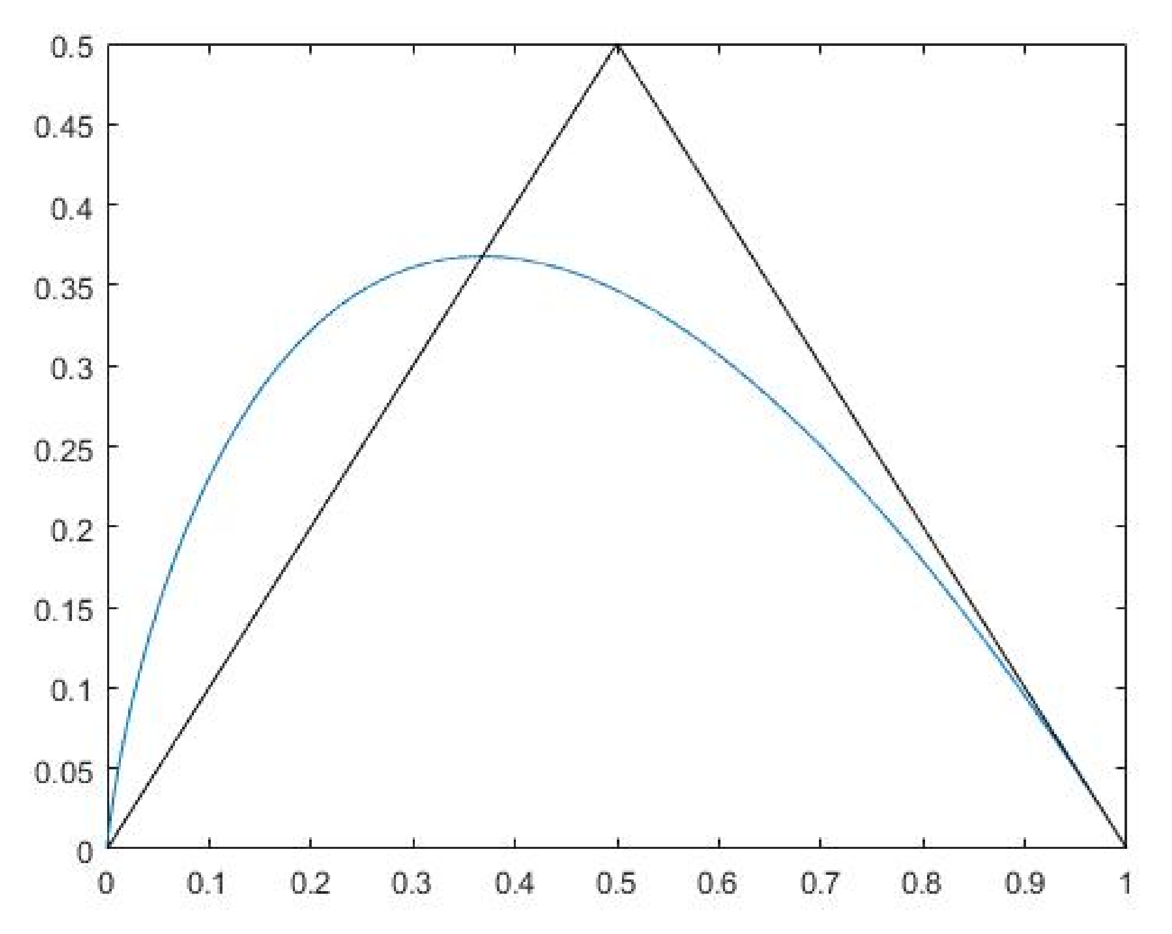
- and have a strong flavor of entropy and for that reason are referred to as entropy in this paper. Being computed on pixel values and not on their distribution, they should not to be considered as similar to entropy, rather they can be thought of as aggregates of pixel values being nonlinearly transformed with , . Here, x stands for or . Up to some normalization, they can be approximated to the average absolute differences between pixel values and . Figure 10 supports this claim by showing on a graph the mapping as a smooth curve and as a triangle function that is fairly similar.
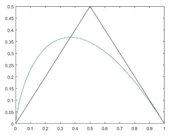 Figure 10. Graph showing some similarity between (the curve line) and (the triangle).
 - and are estimates of the skewness.
For each sample, the features extracted are recorded as a row-vector with the following order.
where , , , and .
The row vectors corresponding to samples in the training set are then stacked into a matrix of size , where each row is related to a specific location and each column is a feature defined by its window, its wavelength, and its equation ranging from (5)–(9). A ground truth label c is assigned to each row and stacked into a column vector of size .
3.3. Classification
The ensemble classifier considered here is an RF. The following three tasks are repeated V times, V being the number of decisions trees to induce.
Rows of , figuring the training instances, are sampled with replacement. This is equivalent to the left multiplication of a matrix of size , where each row contains only one component equal to 1 and its location in the row is evenly drawn from . The assigned labels are also transformed into . Moreover, a random G-sized subset of the -columns is selected. This is equivalent to the right multiplication of of size defined as the identity matrix deprived of a random set of columns. The labels remain unmodified. Finally, is used to train a decision tree using the Classification And Regression Trees (CART) methodology. The trained decision tree maps any row-vector of size into an integer , C being the number of classes.
The predictions of V decision trees are fused according to the majority rule.
where is a row vector, and is equal to one when is true and zero if not.
3.4. Measurements of Feature Importance
As side information, the training of decision trees brings us measurements of feature importance. Let us consider the v-indexed decision tree trained with and denote the number of its internal nodes (including its root node). Considering a specific node indexed by n, from the previous splits, there remains a set of samples and labels which are rows of and , the set of these row indexes is denoted . Components of and are denoted as and . At this node, samples are split upon a feature , which is randomly selected without repetition and a cutting point , defining two complementary subsets.
Splitting modifies the class distribution into and . These class distributions are associated to, respectively, , , and .
The importance of a feature used in node n is here the amount by which splitting reduces entropy.
The relative amount of samples dealt by each node is used as weighting when averaging
The measures of feature importance are defined as
where is a normalization factor here defined as
Note does not take into account to which class each sample is assigned, it assumes that at each leaf, the class predicted is the most likely. The rationale is that a decision tree makes more reliable predictions when training instances reaching a leaf are more often belonging to the same class. Moreover, entropy is precisely measuring that “purity”.
As exemplified in [48], we use feature selection to improve performance and help to prevent the “curse of dimensionality”. As compared to principal component analysis, which is generally used for dimension reduction, the -driven feature selection is expected to be more effective when discriminating between classes. We select the G most important features and train a new model using only those G features, G being a new parameter. To select those features, they are first ranked by increasing order of importance as measured by , and then the first G features are selected.
where are the features in ranked order, and is the selected features. The selection of features is equivalent to the right multiplication of a matrix obtained by removing of the -identity matrix the following columns . The new ensemble classifier is trained as in Section 3.3, but using instead of .
| Algorithm 1: Composite Window Based Feature Extraction Method |
| Input: |
| : multispectral image of size |
| : set of locations of size |
| : set of ground truth labels |
| : size of the smaller window |
| : size of the larger window |
| V: number of decision trees to be trained |
| G: number of features to be sampled for training decision trees |
| : number of features to be selected for training a new ensemble classifier |
| Output: |
| : ensemble classifier |
|
3.5. Precision Evaluation
Three classical evaluation metrics are used here to test a classifier h on a test set for which the true labels are known and denoted .
- : The Overall Accuracy measures the true prediction rate.where is the number of test samples.
- : The kappa-statistic is concerned with the overall accuracy.
- : The per-class accuracy measures the prediction rate when testing only samples of class c.and is the number of test samples belonging to class c.
- : the per-class Area measures the area (in km) correctly detected as of class c.where is the area covered by a pixel.
3.6. Parameter Setting
Two parameters need to be set in RF classifier: the number of decision trees to be generated (Ntree) and the number of variables to be selected and tested for the best split when growing the trees (Mtry). In this study, the default value of 100 for Ntree was used, and the Mtry parameter was set to the square root of the number of input variables. For comparisons purposes, five learning techniques, and , are trained with the same training set and tested on the same test set . Besides, the Blue Mountain Forest is the fire burn area, so differential burn ratio (dNBR) is added to classify the area in this study.
- is an RF trained on spectral features. As in Algorithm, feature preparation (steps 2–7) is replaced by , where and . Moreover, RF training is remained unchanged with steps 9–16, step 14 not included, and using decision trees.
- and are an RF trained on texture features computed using a single window of size, respectively, 3 × 3, 5 × 5 and 7 × 7. As in Algorithm, feature preparation is done with steps 1–9, step 5 not included. RF training is done using with steps 10–16, step 14 not included.
- is an RF trained on texture features computed using a composite window of sizes 5 × 5 and 7 × 7. Feature preparation is done according to steps 1–9 of Algorithm. RF training is done using with steps 10–16, step 14 not included.
The proposed learning technique is described in Algorithm. When applied to Nezer Forest, uses features out of the 40 available. Moreover, for Blue Mountain Forest, features are used out of the 130 available.
4. Experimental Results
4.1. Overall Accuracy Results
Table 3 shows the (overall accuracy) and (Kappa’s statistic) for all six methods , and when tested on Nezer Forest and Blue Mountain Forest. The different methods are nearly always ranked in the same order when measured using or and when applied to both datasets. An increased performance is observed when using texture features: and are better performing than . With respect to the size of the window, performance appears increasing up to a threshold and then decreasing. The threshold seems to be for Nezer forest and for Blue Mountain forest, as among , is best performing on the first dataset and is best performing on the second dataset. Using a composite window proves to be successful on both datasets when compared to using a window having the best performing size, as is increasing the overall accuracy by when compared to on the first dataset, and also when compared to on the second dataset. Performance appears to be further increased when the number of features is reduced. Indeed, when comparing with , the overall accuracy remains unchanged on the first dataset and is increased by on the second dataset. Considering the popularity of dNBR in fire monitoring, it is used to improve classification performance for Blue Mountain Forest data in this study. The corresponding results are shown in Table 3. When dNBR is combined with spectral or texture features for classification, there is no glaringly obvious effect on the improvement of classification performance.

Table 3.
Overall accuracy performance.
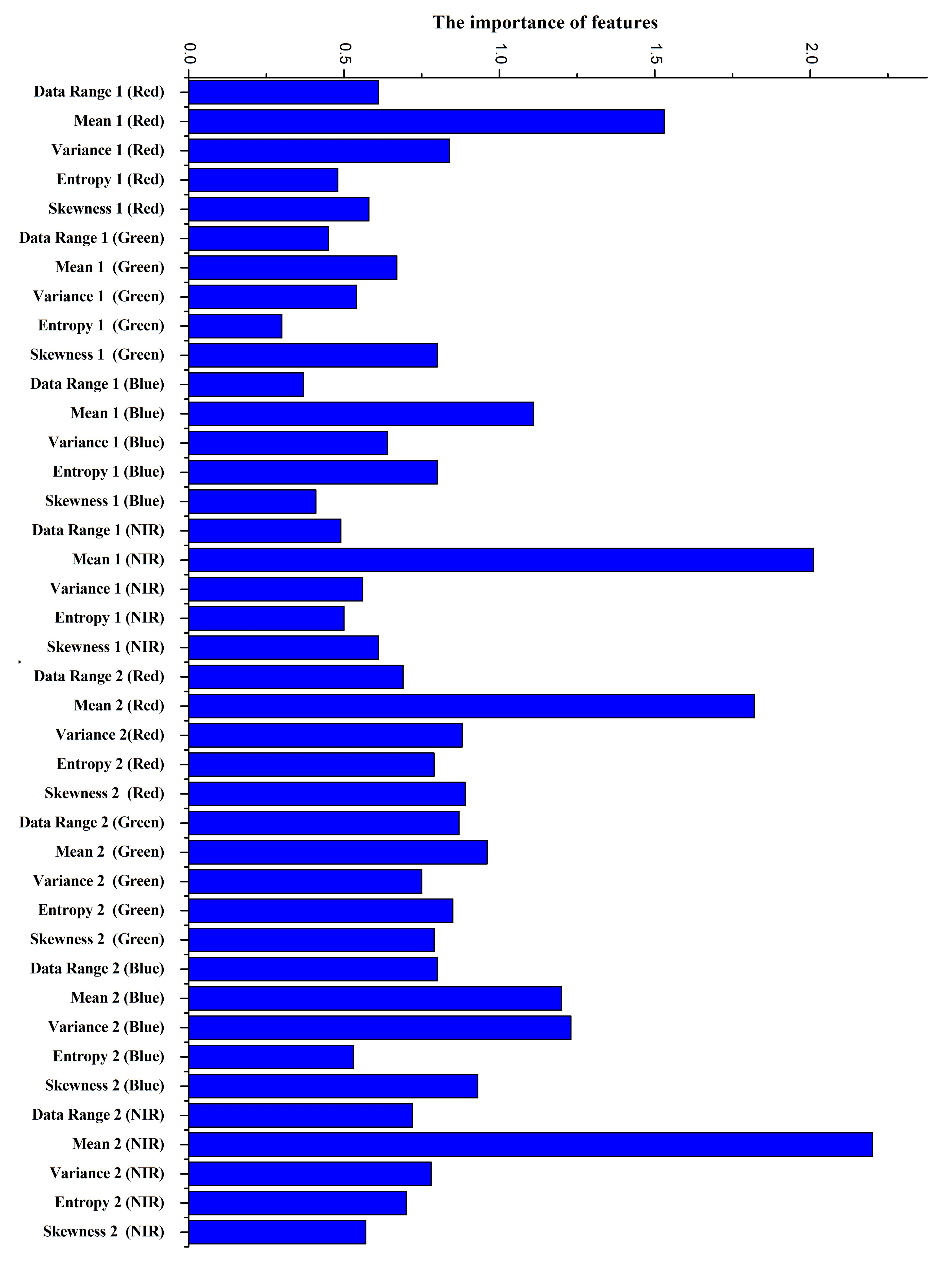
The feature importance measurements obtained on the two studied areas are, respectively, shown in Figure 11 and Figure 12. In Figure 11, the twenty-first features are computed with the smaller window, and the next twenty with the larger window. Moreover, within each twenties, the first five are data range, mean, variance, entropy, and skewness, computed using the red wavelength (630–690 nm), and in the same way the following features are, respectively, accounting for the green (520–600 nm), blue (450–520 nm), and near-infrared (NIR) (760–900 nm) wavelengths. For Nezer forest, the mean appears to be more important in these five types of features. However, with two significant exceptions: skewness computed by the green wavelength, aggregated with the smaller window and variance captured at the blue wavelength using the larger window seem to be more crucial than mean. Among texture features, entropy seems to be least significant in most wavelengths. Entropy is a measure of the amount of information in an image, which indicates the degree of nonuniformity of the texture in the image. When the pixel values in the window are highly random and dispersed, the entropy value is very high. In this study, the entropy of the Nezer Forest is extracted by windows ( and ), which have a small number of pixels. Therefore, entropy has a low contribution to classification.

Figure 11.
Nezer Forest.
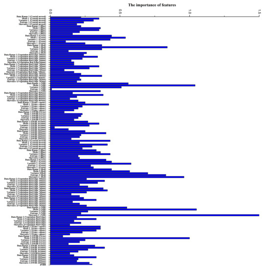
Figure 12.
Blue Mountain Forest.
In Figure 12, the 65 first features are computed with a smaller window, the other 65 features with a larger window. Within each set of features, the first five are data range, mean, variance, entropy, and skewness computed using the coastal aerosol wavelength (442 nm). Similarly, the following features are, respectively, accounting for the blue (492 nm), green (560 nm), red (664 nm), vegetation red (704, 740, and 783 nm), near-infrared (NIR) (832 nm), and subsequent infrared wavelengths (86 nm, 945 nm, 1373 nm, 1614 nm, and 2202 nm). Moreover, dNBR’s feature importance value is shown at the bottom of the figure. For the Blue Mountain Forest, the results show that the relative importance of features to classification is similar to the Nezer Forest. Compared with other features, the mean has a greater contribution to classification in most wavelengths. With the significant exception: skewness computed by the NIR wavelength, aggregated with the larger window makes the greatest contribution to classification.
Besides, for the two sites, whether features are aggregated with the smaller window or with the larger window, seems to have little or no effect on feature importance. Interestingly, greater importance seems assigned to features computed with intensities captured at the NIR wavelength and to a lesser extent at the red wavelength. Some similarities results shown in Figure 5b by [13] indicating that canopy reflectance has much higher values at such wavelengths. The full agreement should not be expected as higher values of reflectance does not necessarily imply higher discriminative power.
4.2. Per-Class Accuracy Performance
Table 4 and Table 5, respectively, show (per-class accuracy) and (per-class area accuracy) achieved by the six models when tested on Nezer Forest and Blue Mountain Forest. Similar trends are displayed with and ; this is no surprise as these metrics are defined with proportional equations in (21) and (22). With respect to Table 3, very similar model comparisons can be drawn, validating our proposed approach: performance is increased when considering texture features when increasing the size of the window up to a threshold, when using a composite window and when appropriately selecting features. Per-class metrics deliver slightly more subtle information: on both datasets, it seems that the optimal window size to use when computing texture features is 5 × 5 for -samples and 7 × 7 for -samples; greater accuracy is displayed for classes for which more training samples are available as compared to the number of test samples, and for those classes, the proposed approach is comparatively showing less increased performance. For Nezer Forest, when using the composite windows (), the accuracy of no-damaged is increased by 1.02% compared to , and the accuracy of damaged is improved by 0.11% compared to . For , the accuracy of no-damaged is improved by 0.32% and the accuracy of damaged is increased by 0.28% compared to . In this study area, the damaged area is 28.48 km, nearly half of the total area. For the Blue Mountain Forest, when the composite window () is used, the accuracy of no-damaged and damaged are, respectively, improved by 0.03% and 0.99% compared to the optimal single window. Compared with the , the accuracy of no-damaged and damaged obtained from are, respectively, increased by 0.01% and 0.82%. The damaged area obtained from is nearly 22.75 km, about half the size of this study area. Besides, when dNBR is combined with spectral or texture features, the classification accuracy improvements of the methods (, , , and ) are not very obvious. More insight is needed to further verify these observations, and to investigate their possible causes.

Table 4.
Classification performance per class of Nezer Forest.

Table 5.
Classification performance per class of Blue Mountain Forest.
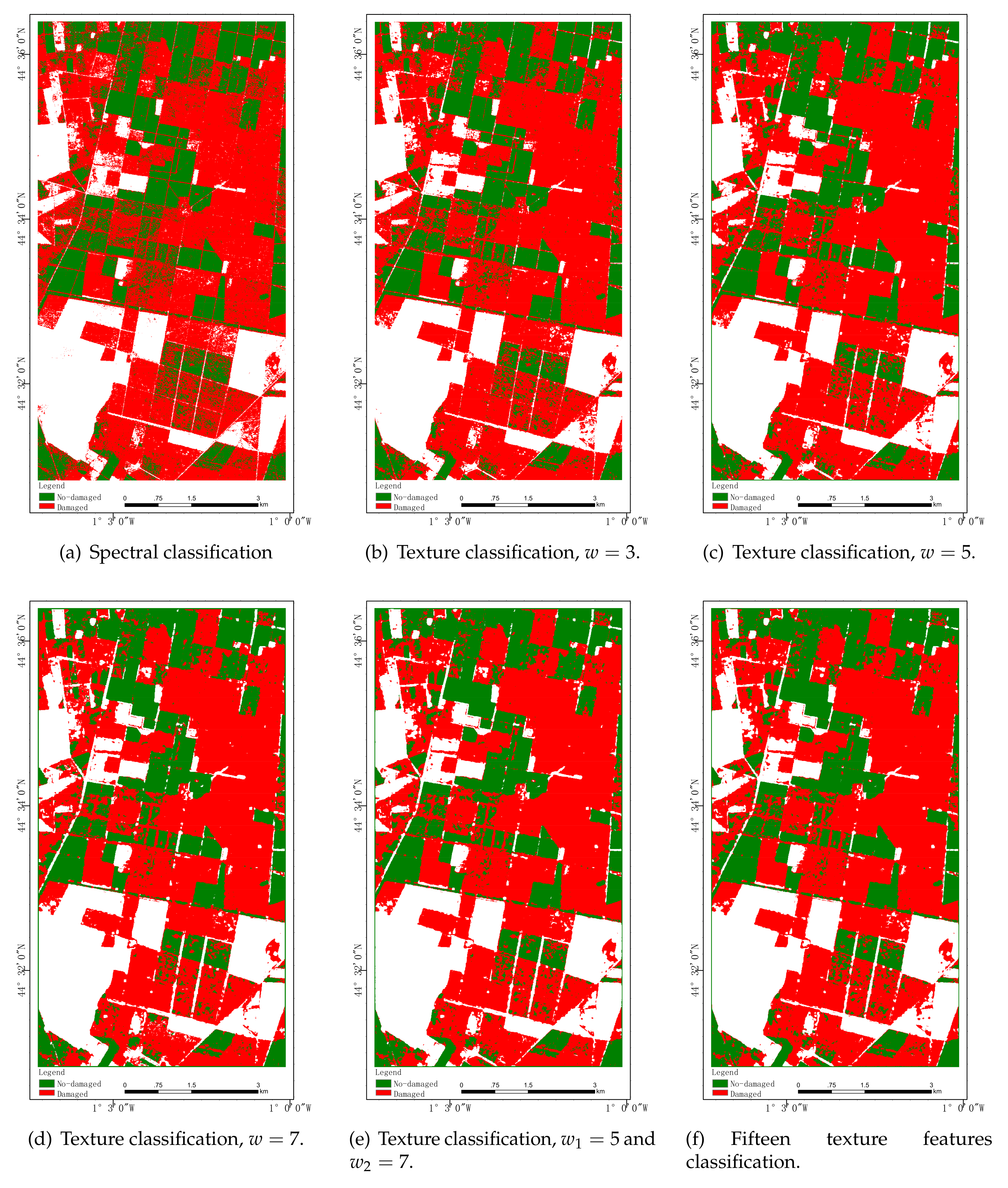
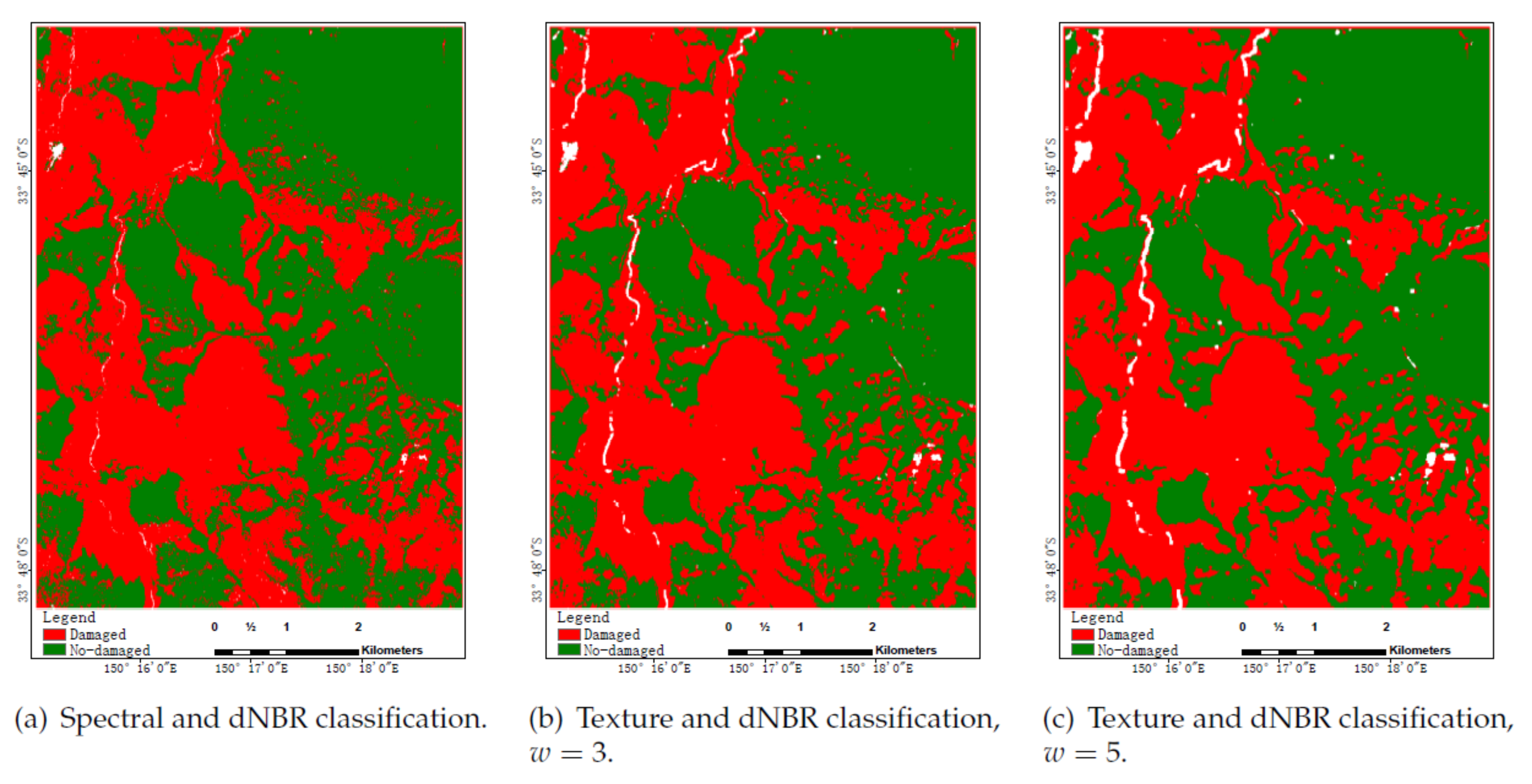
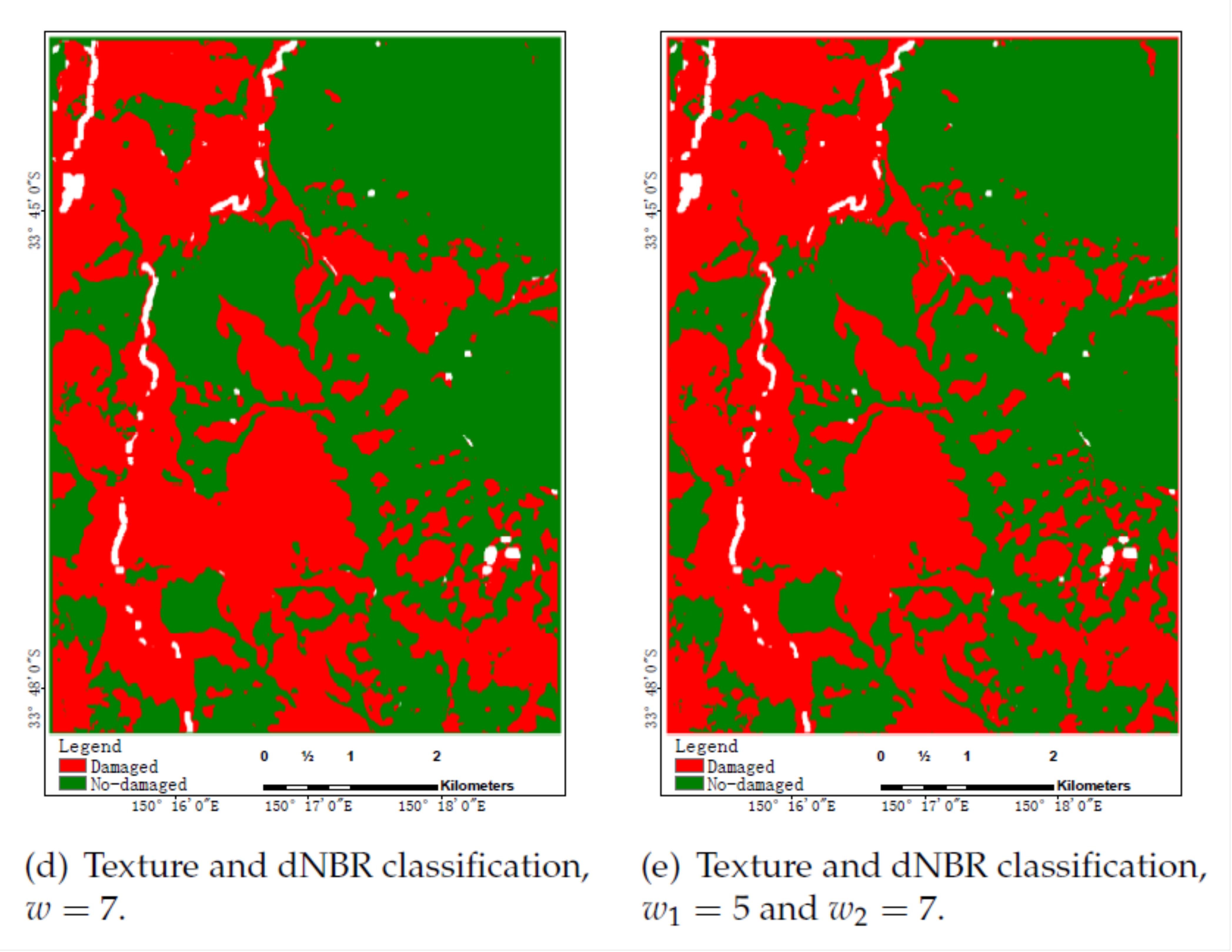
Figure 13,Figure 14 and Figure 15 show classification results in color maps corresponding to the different models when tested on each dataset. Samples classified as , , and are, respectively, displayed in red, green, and white. According to the above analysis of Table 3, Table 4 and Table 5, for three figures, the classification performance is improved from the first figure to the last, among which the last one has the highest classification accuracy and relatively few wrong pixels. Moreover, the color maps obtained by the proposed method(Figure 13f, Figure 14f, and e) are more clear and smooth. Unfortunately, the increases in performance as measured by some accuracy metrics do not translate here in maps easier to interpret, an issue exceeding the scope of this paper.
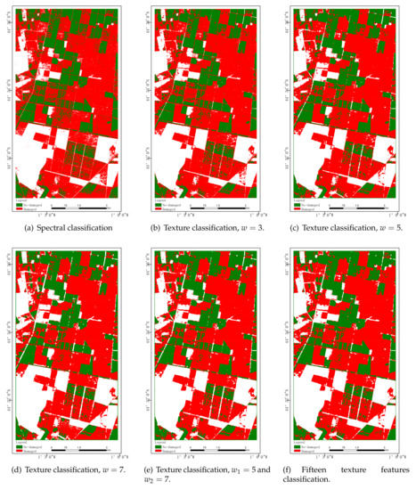
Figure 13.
Nezer forest classification results.
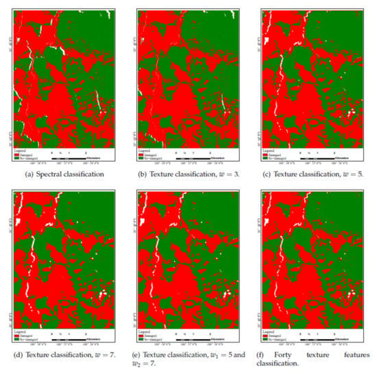
Figure 14.
Blue Mountain Forest classification results.
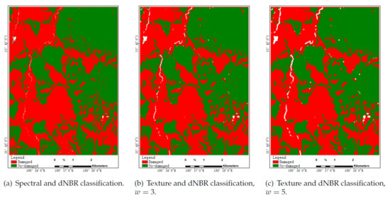
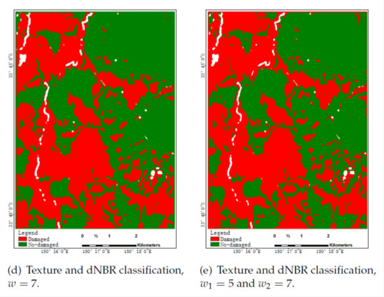
Figure 15.
Blue Mountain Forest classification results using dNBR.
5. Discussion
In this study, we propose a novel texture feature extension method based on the composite windows for the forest disaster monitoring. As a supplementary benefit, the training of random forest provides measurements of feature importance which are used to features selection. The results of the two study areas demonstrate the effectiveness of the proposed method.
- (1)
- In this study, five types of texture features are computed by different sizes of windows. The results of Table 3, Table 4 and Table 5 show that compared with spectral features, texture information contributed to the increased accuracy in the classification of forest detection. This is because the texture features of an image include vital information about the spatial and structural information of objects. In the traditional pixel-based method, pixels are separately classified according to their digital values, but spatial concepts or contextual information are not contained [49]. In this case, the misclassification rate is usually high due to (1) similar spectral features of some classes, and (2) the existence of mixed pixels located at the border between classes. In our study, by incorporating texture features in the classification, different substances with the same spectral features can be distinguished efficiently, and higher classification accuracies can be attained. The studies of Jiang et al. [25] and Kulkarni et al. [27] also demonstrated that texture information has a huge impact on forest disturbance monitoring.
- (2)
- As described in [50], the size of the window is extremely important for the texture features extraction. To find the optimal single window size, different window sizes, including , , and , are used to calculate texture information in our study. The RF classifier is applied to these features derived from three window sizes. The OA and kappa coefficient of the two study areas are displayed in Table 3. This table shows that the highest kappa value and the overall accuracy were obtained at texture window sizes of in the Nezer Forest. Murray et al. [32] and Puissant et al. [34] also used the window sizes of to extract texture features, which proved that this size has advantages for the accurate extraction of texture information. The situation in Blue Mountain Forest is a little different from that in the first area. The significance results show that the overall classification performance is increased from to . Moreover, the performance had a slight dip at a window size of . Because of the different resolution of images and objects, the textures of the degree of thickness are different. Therefore, the optimal window sizes of these two research areas are different.
- (3)
- Although the texture features extracted by a single window contribute to the classification, this method does not adequately consider the scale of different objects. It is of great significance to compound windows of different sizes to cover targets of different sizes. Considering the help of texture information extracted from different optimal windows to improve classification performance, two windows ( and ) with optimal performance are combined in this study. When using the composite window, the classification performance is superior for both study areas. The OA, kappa coefficient, and the pcA have been significantly improved. The main reason is that the composite window not only contains more information, but also can find out precise localizations of boundary edges between adjacent regions.
- (4)
- For the RF classifier, the number of decision trees (Ntree) is set to 500 in many studies, because the errors stabilize before this number of classification trees is achieved [51]. Other researches have also obtained good classification performance by using different values for Ntree such as 100 [52]. In our study, the default value of 100 for Ntree is used for all the methods, and the experimental results show that the OA is over 97% for two study areas. Increasing the value of Ntree to 500 does not greatly improve the classification accuracy, but increases the training time.
- (5)
- In this study, five types of texture features—data range, mean, variance, entropy, and skewness—were computed for all bands. Using all texture features in the RF classifier may not be desirable because of feature redundancy. Some studies show that the feature selection not only reduces classification complexity, but also can enhance classification accuracy [53,54]. In our study, the importance of variables showed in Figure 11 and Figure 12 was obtained by RF. To reduce the feature dimension, we select some features for training according to these two figures. In this study, we used two datasets to test the effects of different variables’ importance thresholds on classification performance. Compared to using all the features, the classification performance is enhanced by using the selected features. Genuer et al. also demonstrated that utilizing RF for variable selection is an effective method [55]. In future studies, we will test the impact of more diverse importance thresholds on classification performance. Moreover, more fire and hurricane data need to test the proposed algorithm.
- (6)
- In this paper, the proposed method is tested on two small data sets. When dNBR is combined with spectral or texture features, the classification accuracies of the methods(, , , and ) are improved a little. Perhaps the research area range is the main reason for the phenomenon. Therefore, a larger study area will be considered to test the effectiveness of the proposed algorithm in our future work.
6. Conclusions
In the context of monitoring forest changes using multispectral images and more specifically texture features, we have investigated two propositions and evaluated them on two multispectral datasets with publicly available ground truths, namely, Nezer Forest and Blue Mountain Forest. The first proposition is the use of two windows, one larger surrounding the other, as an alternative to the classical use of a single sized window, whose size is to be precisely estimated. The discriminative ability of the computed texture features is examined by feeding them into a Random Forest ensemble classifier known to be a performing classifier. The second proposition is to use measurements of feature importance for feature selection, as these are available when training the ensemble classifier, not needing increased computation time. Classifying results show that both propositions have provided an increase in the classification performance when measured with overall accuracy, kappa’s statistic, and per-class accuracy. In the future, a larger range of forest disturbance data is needed to verify the effectiveness of the proposed method. Besides, we recommend extending and testing our approach to other ecosystems, such as the agricultural ecosystem.
Author Contributions
Y.Q. and W.F. conceived and designed the experiments. X.Z. performed the experiments and wrote the paper. W.F. and G.D. revised the paper. L.G. and M.X. edited the manuscript. All authors reviewed and approved the final manuscript.
Funding
This work is supported by the National Natural Science Foundation of China (61772397), the National Key R&D Program of China (2016YFE0200400), and the Open Research Fund of Key Laboratory of Digital Earth Science (2019LDE005).
Acknowledgments
Access to the images was granted by the CNES Kalideos Programme (http://Kalideos.cnes.fr).
Conflicts of Interest
The authors declare no conflict of interest.
References
- De Luis, M.; González-Hidalgo, J.; Raventós, J. Effects of fire and torrential rainfall on erosion in a Mediterranean gorse community. Land Degrad. Dev. 2003, 14, 203–213. [Google Scholar] [CrossRef]
- Ochego, H. Application of remote sensing in deforestation monitoring: A case study of the Aberdares (Kenya). In Proceedings of the 2nd FIG Regional Conference, Marrakech, Morocco, 2–5 December 2003. [Google Scholar]
- Christopoulou, A.; Mallinis, G.; Vassilakis, E.; Farangitakis, G.P.; Arianoutsou, M. Assessing the impact of different landscape features on post-fire forest recovery with multitemporal remote sensing data: The case of Mount Taygetos (southern Greece). Int. J. Wildland Fire 2019, 28, 521–532. [Google Scholar] [CrossRef]
- Foster, D.R. Species and stand response to catastrophic wind in central New England, USA. J. Ecol. 1988, 76, 135–151. [Google Scholar] [CrossRef]
- Boutet, J.C.; Weishampel, J.F. Spatial pattern analysis of pre-and post-hurricane forest canopy structure in North Carolina, USA. Landsc. Ecol. 2003, 18, 553–559. [Google Scholar] [CrossRef]
- Chaparro, D.; Vall-Llossera, M.; Piles, M.; Camps, A.; Rüdiger, C.; Riera-Tatché, R. Predicting the extent of wildfires using remotely sensed soil moisture and temperature trends. IEEE J. Sel. Top. Appl. Earth Obs. Remote. Sens. 2016, 9, 2818–2829. [Google Scholar] [CrossRef]
- Abdollahi, M.; Dewan, A.; Hassan, Q.K. Applicability of Remote Sensing-Based Vegetation Water Content in Modeling Lightning-Caused Forest Fire Occurrences. Int. J. Geo Inf. 2019, 8, 143. [Google Scholar] [CrossRef]
- Ahmed, M.R.; Hassan, Q.K.; Abdollahi, M.; Gupta, A. Introducing a New Remote Sensing-Based Model for Forecasting Forest Fire Danger Conditions at a Four-Day Scale. Remote Sens. 2019, 11, 2101. [Google Scholar] [CrossRef]
- Morton, D.C.; DeFries, R.S.; Nagol, J.; Souza, C.M., Jr.; Kasischke, E.S.; Hurtt, G.C.; Dubayah, R. Mapping canopy damage from understory fires in Amazon forests using annual time series of Landsat and MODIS data. Remote Sens. Environ. 2011, 115, 1706–1720. [Google Scholar] [CrossRef]
- FAO; UNEP. The State of the World’s Forests 2020: Forests, Biodiversity and People; FAO: Rome, Italy, 2020. [Google Scholar]
- Camarretta, N.; Harrison, P.A.; Bailey, T.G.; Potts, B.M.; Hunt, M.A. Monitoring forest structure to guide adaptive management of forest restoration: A review of remote sensing approaches. New For. 2020, 51, 573–596. [Google Scholar] [CrossRef]
- Serbin, S.P.; Ahl, D.E.; Gower, S.T. Spatial and temporal validation of the MODIS LAI and FPAR products across a boreal forest wildfire chronosequence. Remote Sens. Environ. 2013, 133, 71–84. [Google Scholar] [CrossRef]
- Meng, R.; Wu, J.; Zhao, F.; Cook, B.D.; Hanavan, R.P.; Serbin, S.P. Measuring short-term post-fire forest recovery across a burn severity gradient in a mixed pine-oak forest using multi-sensor remote sensing techniques. Remote Sens. Environ. 2018, 210, 282–296. [Google Scholar] [CrossRef]
- Chehata, N.; Orny, C.; Boukir, S.; Guyon, D. Object-based change detection in wind-storm damaged forest using high resolution multispectral images. Int. J. Remote Sens. 2014, 35, 4758–4777. [Google Scholar] [CrossRef]
- Ahmad, F.; Goparaju, L. Analysis of forest fire and climate variability using Geospatial Technology for the State of Telangana, India. Environ. Socio Econ. Stud. 2019, 7, 24–37. [Google Scholar] [CrossRef]
- Thyagharajan, K.K.; Vignesh, T. Soft Computing Techniques for Land Use and Land Cover Monitoring with Multispectral Remote Sensing Images: A Review. Arch. Comput. Methods Eng. 2019, 26, 275–301. [Google Scholar] [CrossRef]
- Wang, S.; Gao, J.; Zhuang, Q.; Lu, Y.; Jin, X. Multispectral Remote Sensing Data Are Effective and Robust in Mapping Regional Forest Soil Organic Carbon Stocks in a Northeast Forest Region in China. Remote Sens. 2020, 12, 393. [Google Scholar] [CrossRef]
- Cohen, W.B.; Yang, Z.; Healey, S.P.; Kennedy, R.E.; Gorelick, N. A LandTrendr multispectral ensemble for forest disturbance detection. Remote Sens. Environ. 2018, 205, 131–140. [Google Scholar] [CrossRef]
- Fokeng, R.M.; Forje, W.G.; Meli, V.M.; Bodzemo, B.N. Multi-Temporal Forest Cover Change Detection in the Metchie-Ngoum Protection Forest Reserve, West Region of Cameroon. Egypt. J. Remote Sens. Space Sci. 2019, 23, 113–124. [Google Scholar] [CrossRef]
- Zarco-Tejada, P.; Hornero, A.; Hernández-Clemente, R.; Beck, P. Understanding the temporal dimension of the red-edge spectral region for forest decline detection using high-resolution hyperspectral and Sentinel-2a imagery. ISPRS J. Photogramm. Remote Sens. 2018, 137, 134–148. [Google Scholar] [CrossRef]
- White, J.C.; Saarinen, N.; Kankare, V.; Wulder, M.A.; Hermosilla, T.; Coops, N.C.; Pickell, P.D.; Holopainen, M.; Hyyppä, J.; Vastaranta, M. Confirmation of post-harvest spectral recovery from Landsat time series using measures of forest cover and height derived from airborne laser scanning data. Remote Sens. Environ. 2018, 216, 262–275. [Google Scholar] [CrossRef]
- Bar, S.; Parida, B.R.; Pandey, A.C. Landsat-8 and Sentinel-2 based Forest fire burn area mapping using machine learning algorithms on GEE cloud platform over Uttarakhand, Western Himalaya. Remote Sens. Appl. Soc. Environ. 2020, 18, 100324. [Google Scholar] [CrossRef]
- Salas, E.A.L.; Boykin, K.G.; Valdez, R. Multispectral and texture feature application in image-object analysis of summer vegetation in Eastern Tajikistan Pamirs. Remote Sens. 2016, 8, 78. [Google Scholar] [CrossRef]
- Zhang, H.; Li, Q.; Liu, J.; Shang, J.; Du, X.; McNairn, H.; Champagne, C.; Dong, T.; Liu, M. Image classification using rapideye data: Integration of spectral and textual features in a random forest classifier. IEEE J. Sel. Top. Appl. Earth Obs. Remote Sens. 2017, 10, 5334–5349. [Google Scholar] [CrossRef]
- Jiang, W.; Rule, H.; Ziyue, X.; Ning, H. Forest fire smog feature extraction based on Pulse-Coupled neural network. In Proceedings of the 2011 6th IEEE Joint International Information Technology and Artificial Intelligence Conference, Chongqing, China, 20–22 August 2011; pp. 186–189. [Google Scholar]
- Benjamin, S.G.; Radhakrishnan, B.; Nidhin, T.; Suresh, L.P. Extraction of fire region from forest fire images using color rules and texture analysis. In Proceedings of the 2016 International Conference on Emerging Technological Trends (ICETT), Kollam, India, 21–22 October 2016; pp. 1–7. [Google Scholar]
- Kulkarni, A. Evaluation of the Impacts of Hurricane Hugo on the Land Cover of Francis Marion National Forest, South Carolina Using Remote Sensing. Master’s Thesis, Louisiana State University, Baton Rouge, LA, USA, 2004. [Google Scholar]
- Akar, Ö.; Güngör, O. Integrating multiple texture methods and NDVI to the Random Forest classification algorithm to detect tea and hazelnut plantation areas in northeast Turkey. Int. J. Remote Sens. 2015, 36, 442–464. [Google Scholar] [CrossRef]
- Li, Y.; Gong, J.; Wang, D.; An, L.; Li, R. Sloping farmland identification using hierarchical classification in the Xi-He region of China. Int. J. Remote Sens. 2013, 34, 545–562. [Google Scholar] [CrossRef]
- Puig, D.; García, M.A. Determining optimal window size for texture feature extraction methods. In Proceedings of the IX Spanish Symposium on Pattern Recognition and Image Analysis, Castellon, Spain, 16–18 May 2001; Volume 2, pp. 237–242. [Google Scholar]
- Marceau, D.J.; Howarth, P.J.; Dubois, J.M.M.; Gratton, D.J. Evaluation of the grey-level co-occurrence matrix method for land-cover classification using SPOT imagery. IEEE Trans. Geosci. Remote Sens. 1990, 28, 513–519. [Google Scholar] [CrossRef]
- Murray, H.; Lucieer, A.; Williams, R. Texture-based classification of sub-Antarctic vegetation communities on Heard Island. Int. J. Appl. Earth Obs. Geoinf. 2010, 12, 138–149. [Google Scholar] [CrossRef]
- Garcia-Sevilla, P.; Petrou, M. Analysis of irregularly shaped texture regions: A comparative study. In Proceedings of the 15th International Conference on Pattern Recognition (ICPR-2000), Barcelona, Spain, 3–7 September 2000; Volume 3, pp. 1068–1071. [Google Scholar]
- Puissant, A.; Hirsch, J.; Weber, C. The utility of texture analysis to improve per-pixel classification for high to very high spatial resolution imagery. Int. J. Remote Sens. 2005, 26, 733–745. [Google Scholar] [CrossRef]
- Dietterich, T. An Experimental Comparison of Three Methods for Constructing Ensembles of Decision Trees: Bagging, Boosting, and Randomization. Mach. Learn. 2000, 40, 139–157. [Google Scholar] [CrossRef]
- Feng, W. Investigation of Training Data Issues in Ensemble Classification Based on Margin Concept. Application to Land Cover Mapping. Ph.D. Thesis, University of Bordeaux 3, Pessac, France, 2017. [Google Scholar]
- Feng, W.; Dauphin, G.; Huang, W.; Quan, Y.; Liao, W. New margin-based subsampling iterative technique in modified random forests for classification. Knowl. Based Syst. 2019, 182, 104845. [Google Scholar] [CrossRef]
- Feng, W.; Dauphin, G.; Huang, W.; Quan, Y.; Bao, W.; Wu, M.; Li, Q. Dynamic Synthetic Minority Over-Sampling Technique-Based Rotation Forest for the Classification of Imbalanced Hyperspectral Data. IEEE J. Sel. Top. Appl. Earth Obs. Remote Sens. 2019, 12, 2159–2169. [Google Scholar] [CrossRef]
- Feng, W.; Huang, W.; Ren, J. Class Imbalance Ensemble Learning Based on the Margin Theory. Appl. Sci. 2018, 8, 815. [Google Scholar] [CrossRef]
- Li, Q.; Feng, W.; Quan, Y.H. Trend and forecasting of the COVID-19 outbreak in China. J. Infect. 2020, 80, 469–496. [Google Scholar] [PubMed]
- Breiman, L.; Friedman, J.; Olshen, R.; Stone, C. Classification and Regression Trees; Wadsworth and Brooks: Monterey, CA, USA, 1984. [Google Scholar]
- Einzmann, K.; Immitzer, M.; Böck, S.; Bauer, O.; Schmitt, A.; Atzberger, C. Windthrow detection in European forests with very high-resolution optical data. Forests 2017, 8, 21. [Google Scholar] [CrossRef]
- Ramo, R.; Chuvieco, E. Developing a random forest algorithm for MODIS global burned area classification. Remote Sens. 2017, 9, 1193. [Google Scholar] [CrossRef]
- Virot, E.; Ponomarenko, A.; Dehandschoewercker, É.; Quéré, D.; Clanet, C. Critical wind speed at which trees break. Phys. Rev. E 2016, 93, 023001. [Google Scholar] [CrossRef]
- Nicolas, J.P. Comm. Affair. Econ. 2009. Available online: https://doi.org/10.1103/PhysRevE.93.023001 (accessed on 14 January 2020).
- National Inventaire Forestier National. Tempete Klaus du 24 Janvier 2009; Inventaire Forestier National: Paris, France, 2009. [Google Scholar]
- ’It’s Heart-Wrenching’: 80 Pecent of Blue Mountains and 50 Pecent of Gondwana Rainforests Burn in Bushfires. Available online: https://www.theguardian.com/environment/2020/jan/17/its-heart-wrenching-80-of-blue-mountains-and-50-of-gondwana-rainforests-burn-in-bushfires (accessed on 28 June 2020).
- Wang, Z.; Zhang, Y.; Chen, Z.; Yang, H.; Sun, Y.; Kang, J.; Yang, Y.; Liang, X. Application of ReliefF algorithm to selecting feature sets for classification of high resolution remote sensing image. In Proceedings of the 2016 IEEE International Geoscience and Remote Sensing Symposium (IGARSS), Beijing, China, 10–15 July 2016; pp. 755–758. [Google Scholar]
- Peña-Barragán, J.M.; Ngugi, M.K.; Plant, R.E.; Six, J. Object-based crop identification using multiple vegetation indices, textural features and crop phenology. Remote Sens. Environ. 2011, 115, 1301–1316. [Google Scholar] [CrossRef]
- Franklin, S.; Hall, R.; Moskal, L.; Maudie, A.; Lavigne, M. Incorporating texture into classification of forest species composition from airborne multispectral images. Int. J. Remote Sens. 2000, 21, 61–79. [Google Scholar] [CrossRef]
- Lawrence, R.L.; Wood, S.D.; Sheley, R.L. Mapping invasive plants using hyperspectral imagery and Breiman Cutler classifications (RandomForest). Remote Sens. Environ. 2006, 100, 356–362. [Google Scholar] [CrossRef]
- Guan, D.; Yuan, W.; Shen, L. Class noise detection by multiple voting. In Proceedings of the 2013 Ninth International Conference on Natural Computation (ICNC), Shenyang, China, 23–25 July 2013; pp. 906–911. [Google Scholar]
- Guyon, I.; Elisseeff, A. An introduction to variable and feature selection. J. Mach. Learn. Res. 2003, 3, 1157–1182. [Google Scholar]
- Dash, M.; Liu, H. Feature selection for classification. Intell. Data Anal. 1997, 1, 131–156. [Google Scholar] [CrossRef]
- Genuer, R.; Poggi, J.M.; Tuleau-Malot, C. Variable selection using random forests. Pattern Recognit. Lett. 2010, 31, 2225–2236. [Google Scholar] [CrossRef]
© 2020 by the authors. Licensee MDPI, Basel, Switzerland. This article is an open access article distributed under the terms and conditions of the Creative Commons Attribution (CC BY) license (http://creativecommons.org/licenses/by/4.0/).


