Author Contributions
Conceptualization, N.H.Q., C.R.H., L.C.S., and L.T.V.H.; Methodology, N.H.Q., L.C.S., R.C., and C.H.Q.; Field investigation, D.V.T., R.C., C.R.H., and N.H.Q.; Data analysis, N.H.Q., P.T.T.N., C.H.Q., D.V.T., and L.T.V.H.; Writing—original draft preparation, N.H.Q.; Writing—review and editing, N.H.Q., C.R.H., C.H.Q., L.C.S., P.T.T.N, L.T.V.H., R.C., and D.V.T; Visualization, N.H.Q., R.C., and C.R.H.; Supervision, C.H.Q., L.C.S., P.T.T.N., and L.T.V.H.; Project administration, C.H.Q. and L.T.V.H. All authors have read and agreed to the published version of the manuscript.
Figure 1.
Location of Thuy Truong commune (central coordinates of 106°38′00E and 20°36′00N) and in situ ground-truth investigation of mangrove locations. Plots for different types (yellow diamonds) and ages (blue diamonds) were positioned with confirmation of the local people. A GPS (Garmin Montana 680) with an integrated 5 M camera was used to locate and photograph each mangrove type and age. The SPOT-7 panchromatic band with the digital number ranged from 0 to 3946 was used for the base map.
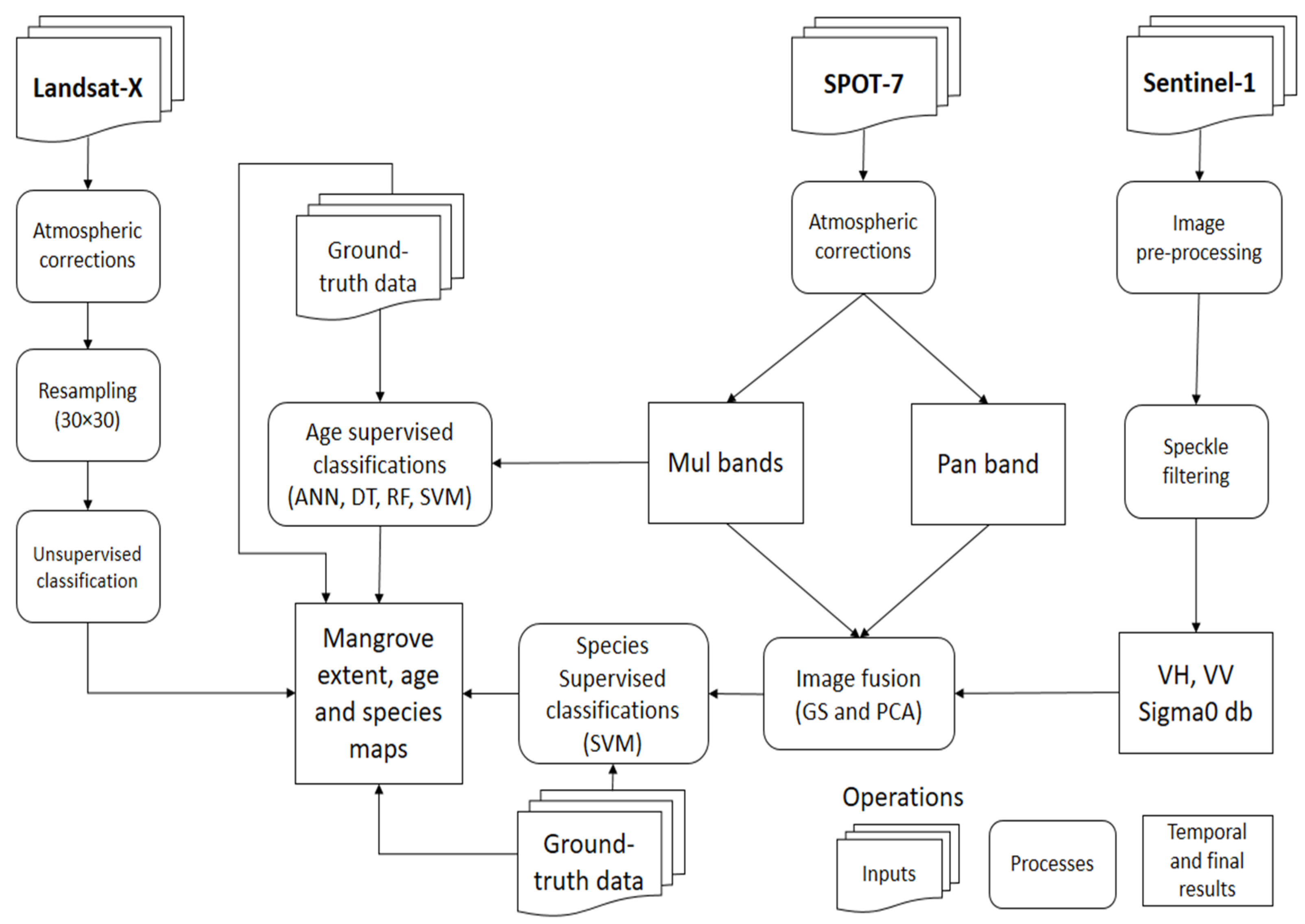
Figure 2.
Flowchart of methodology used for mapping mangrove extent, age, and species. X refers to the mission number of the used Landsat images; ANN, DT, RF, SVM stand for artificial neural network, decision tree, random forest, and support vector machine, respectively; Mul and Pan are short forms of multispectral and panchromatic bands, respectively; GS and PCA indicate Gram–Schmidt and principal component analysis image fusion methods; V and H are vertical and horizontal, respectively, and coupled letters of VH and VV indicate Synthetic Aperture Radar (SAR) cross-polarizations.
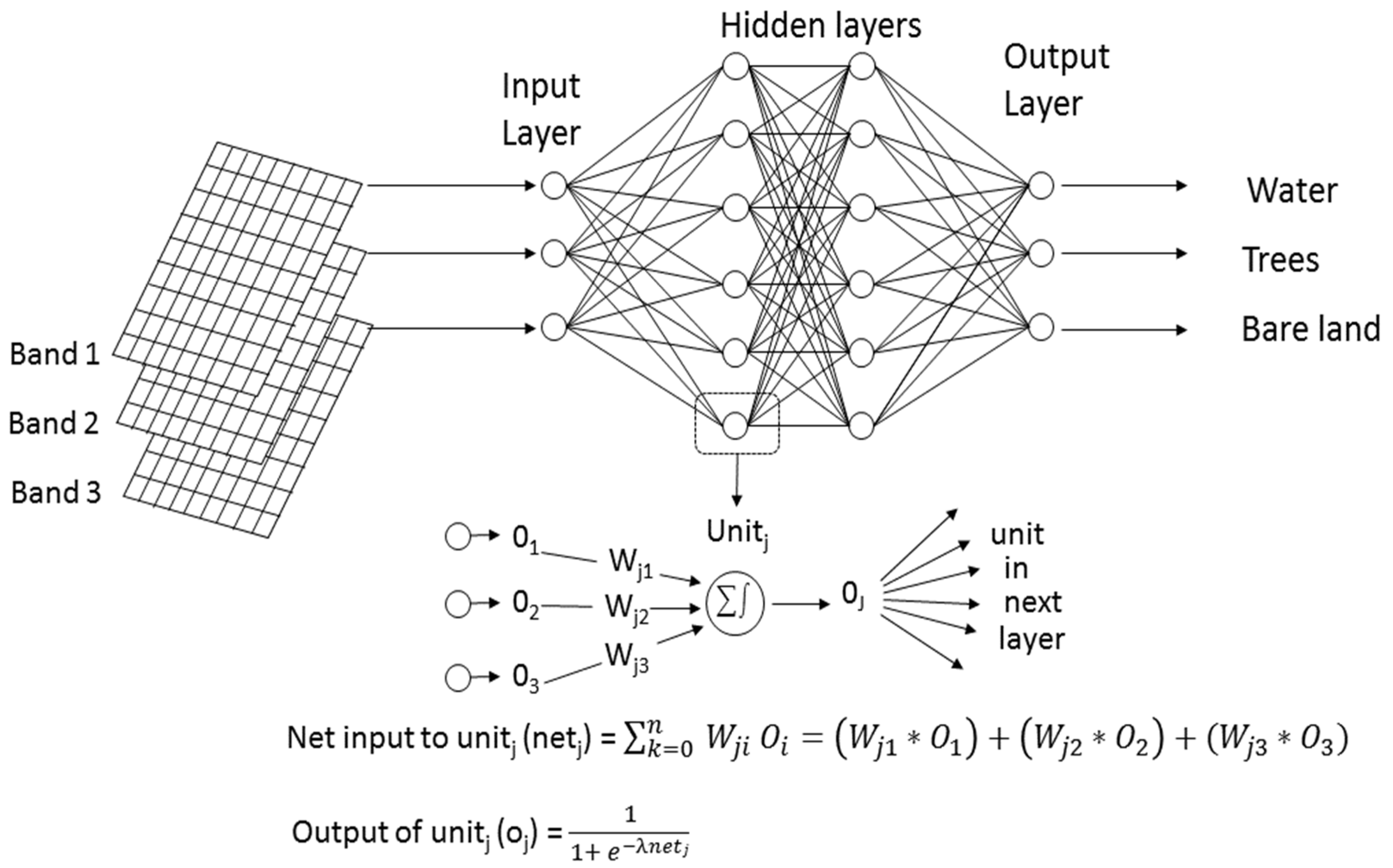
Figure 3.
Classification of remote sensing data by an artificial neural network (adapted from Foody 1996) where Wij is the weight that connects the jth unit with its ith incoming connection; Oi and Oj are the value of the ith incoming connection and jth output connection; and λ is a gain parameter, which is often set to 1.
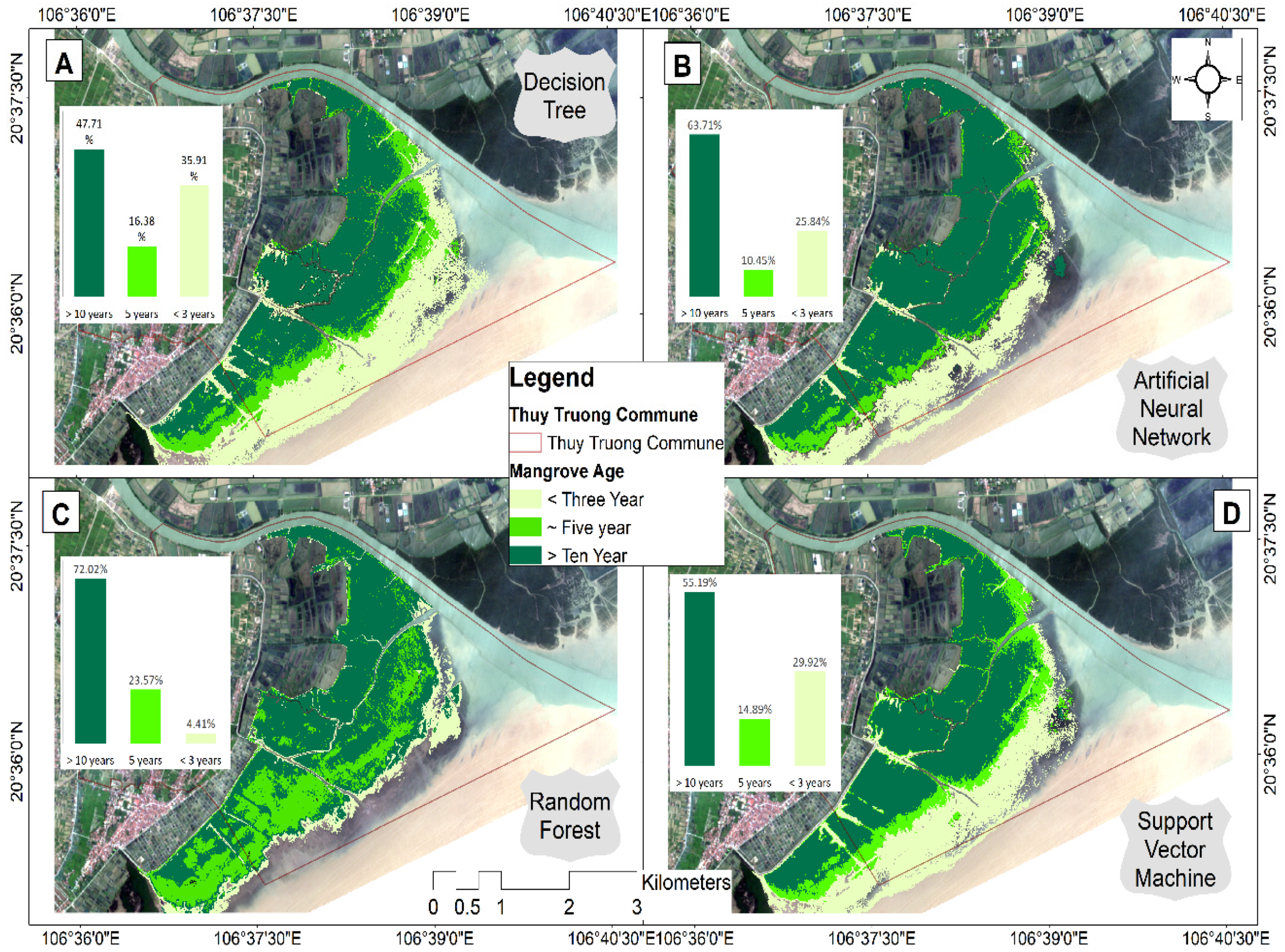
Figure 4.
Maps of classifications using the multispectral data of SPOT-7 acquired on 17 May 2019 for mangroves of ages older than 10 years, around five years, and younger than three years, mapped for the four classifiers of decision tree (A), artificial neural network (B), random forest (C), and support vector machine (D). The background is the SPOT-7 true-color composition image and the red polygon shows the border of the Thuy Truong commune.
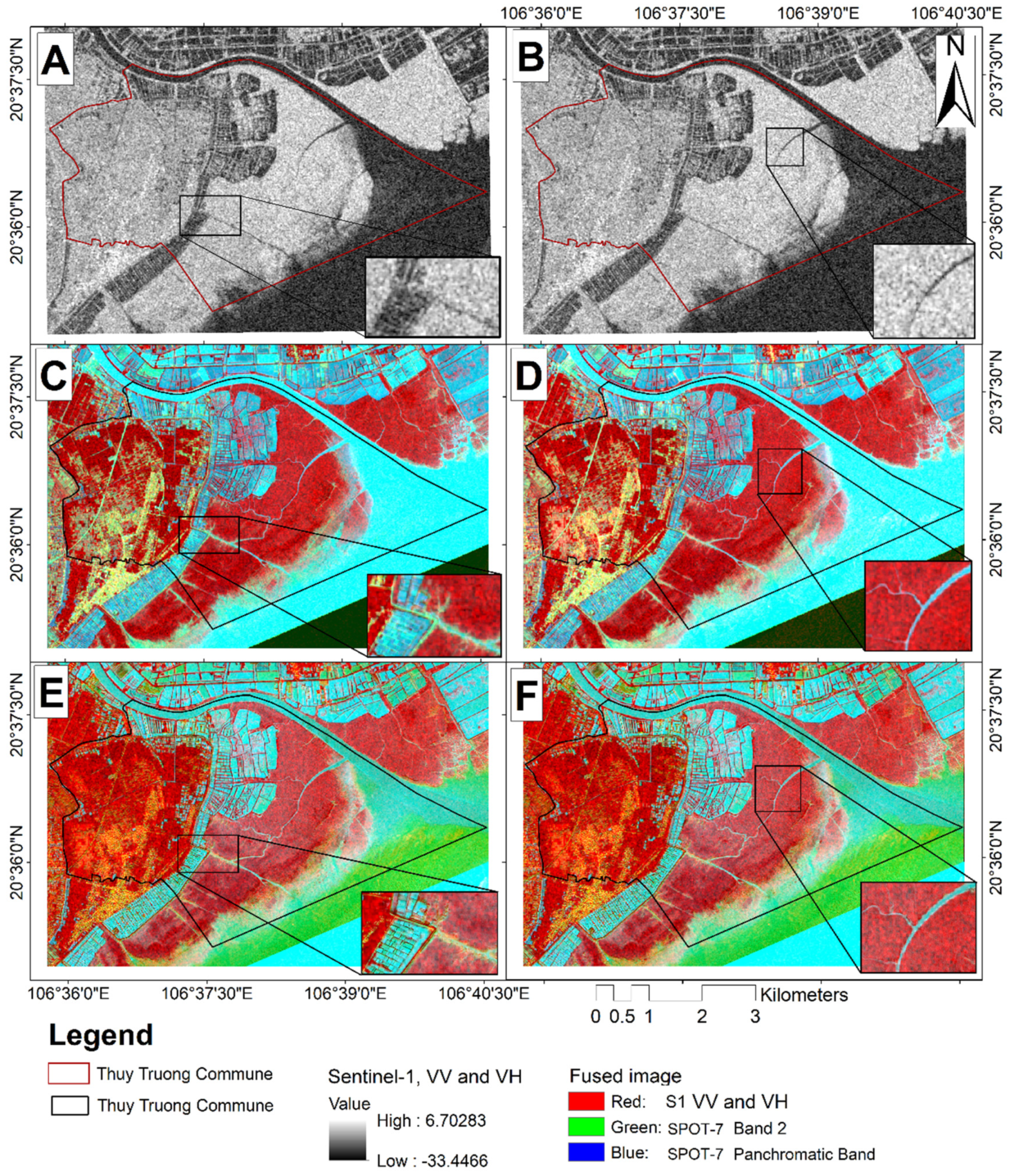
Figure 5.
Demonstrations of SPOT-7 and Sentinel-1 (S1) image fusion processes where (A) is the original Sentinel-1 VH layer and (B) is Sentinel-1 VV layer (sigma0 in decibel); and (C–F) depict the results of the fused images using VH–GS, VV–GS, VH–PCA, and VV–PCA, respectively.
Figure 5.
Demonstrations of SPOT-7 and Sentinel-1 (S1) image fusion processes where (A) is the original Sentinel-1 VH layer and (B) is Sentinel-1 VV layer (sigma0 in decibel); and (C–F) depict the results of the fused images using VH–GS, VV–GS, VH–PCA, and VV–PCA, respectively.
Figure 6.
Maps of classified mangrove species; GS and PCA indicate Gram–Schmidt and principal component analysis image fusion methods; V and H are vertical and horizontal, respectively and coupled letters of VH and VV indicate SAR cross-polarizations. VH_GS, VH_PCA, VV_GS, and VV_PCA are combinations of fused images of SPOT-7 acquired on 17 May 2019 and Sentinel-1 polarization data (VH or VV) and the image fusion methods (GS or PCA).
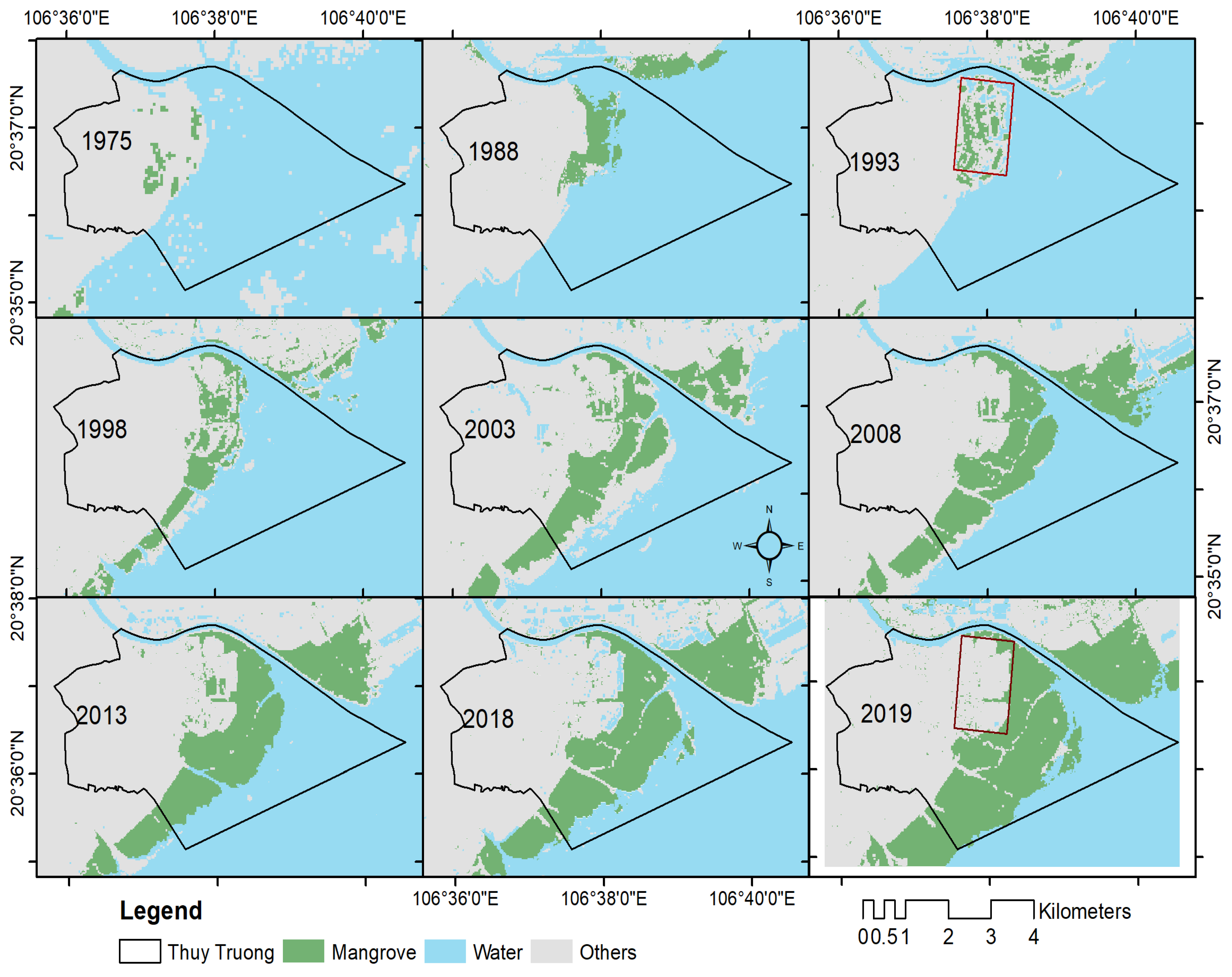
Figure 7.
Changes in mangrove extent from 1975 to 2019 classified from a time series of Landsat images missions 2 to 8 (described in the
Table 2) using the iterative self-organizing data analysis technique (ISODATA) classification, an unsupervised image classification approach (detailed in
Section 2.3.1). The red rectangle denotes the same area of intensive aquaculture in 1993 and 2019.
Figure 8.
Total mangrove area (orange line) and changes in extent (blue line) (ha) from 1975–2019 in Thuy Truong commune.
Figure 8.
Total mangrove area (orange line) and changes in extent (blue line) (ha) from 1975–2019 in Thuy Truong commune.
Figure 9.
Sentinel-1 VH and VV backscatters on different land use and land cover; training data were used for (A) mangrove age and (B) mangrove species; V and H are vertical and horizontal, respectively, and coupled letters of VH and VV indicate SAR cross-polarizations.
Figure 9.
Sentinel-1 VH and VV backscatters on different land use and land cover; training data were used for (A) mangrove age and (B) mangrove species; V and H are vertical and horizontal, respectively, and coupled letters of VH and VV indicate SAR cross-polarizations.
Figure 10.
Pictures of three mangrove species taken by the authors in Thuy Truong commune on 22 November 2018.
Figure 10.
Pictures of three mangrove species taken by the authors in Thuy Truong commune on 22 November 2018.
Table 1.
In situ data for supervised remote sensing image classifications and accuracy evaluation. Examples of three existing mangrove species with scientific names, local names are marked in bold for illustration.
Table 1.
In situ data for supervised remote sensing image classifications and accuracy evaluation. Examples of three existing mangrove species with scientific names, local names are marked in bold for illustration.
| Training for Mangrove Type | Number of Polygons | Average Area (ha) | Sum Area (ha) | Training for Mangrove Age | Number of Polygons | Average Area (ha) | Sum Area (ha) |
|---|
| Agriculture | 8 | 1.6 | 12.4 | Agriculture | 10 | 1.9 | 18.8 |
| Aquaculture | 6 | 1.7 | 10.1 | Aquaculture | 12 | 2.2 | 26.3 |
| Seawater | 4 | 21.5 | 86.1 | Seawater | 5 | 2.5 | 12.4 |
| Bare land | 6 | 0.4 | 2.3 | Bare land | 14 | 0.2 | 3.2 |
| Residence | 6 | 0.9 | 5.1 | Residence | 6 | 1.1 | 6.5 |
| River | 7 | 3.9 | 27.4 | River | 8 | 1.8 | 14.4 |
| Road | 7 | 0.1 | 0.6 | Road | 13 | 0.4 | 5.0 |
| Sonneratia caseolaris (ban) | 9 | 2.1 | 18.9 | >10 year mangrove | 16 | 1.9 | 30.4 |
| Aegiceras corniculatum (Su) | 9 | 1.3 | 11.3 | 5 year mangrove | 10 | 1.2 | 11.7 |
| Kandelia obovata (Vet) | 16 | 0.5 | 7.4 | <3 year mangrove | 11 | 1.2 | 13.1 |
| Sum | 78 (23) | | 181.6 | | 105 (32) | | 141.6 |
Table 2.
Summary of remote sensing data used (X refers to the Landsat mission of 2, 5, and 8; L1TP is data processing level 1 with precision terrain corrected; BQA stands for band quality; MSS is Multispectral Scanner Sensor; TM stands form; OLI is Operational Land Imager; Mul and Pan are short for multispectral and panchromatic bands, respectively; GPL is geometric processing level; RPL is radiometric processing level; and GRD is ground-range detected. V and H are vertical and horizontal, respectively, and coupled letters of VH and VV indicate SAR cross-polarizations).
| Data | Time of Acquisition | Level | Band and Polarization | Resolution |
|---|
| Landsat (X) | 1975/04/20 (2MSS), 1988/11/04 (5TM), 1993/11/02 (5TM), 1998/10/15 (5TM), 2003/10/10 (5TM), 2008/11/11 (5TM), 2013/10/08 (8OLI), 2018/10/06 (8OLI), 2019/05/18 (8OLI) | (2) L1TP, (5) L1TP, (5) L1TP, (5) L1TP, (5) L1TP, (5) L1TP, (8) L1TP, (8) L1TP, (8) L1TP, | (2) 4–6, (5) 1–7, BQA, (5) 1–7, BQA, (5) 1–7, BQA, (5) 1–7, BQA, (5) 1–7, BQA, (8) 1–11, BQA, (8) 1–11, BQA, (8) 1–11, BQA. | (2) 60 m (5) 30 m (5) 30 m (5) 30 m (5) 30 m (5) 30 m (8) 30 m, Pan (B8)15 m (8) 30 m, Pan (B8)15 m (8) 30 m, Pan (B8)15 m |
| SPOT-7 | 2019/05/17 | GPL: Sensor RPL: Basic | Band 0–3 (Mul) Pan | Mul 6 m Pan 1.5 m |
| Sentinel-1 | 2019/05/16 (ascending) | L1 GRD product | VH and VV | 10 m |
Table 3.
Accuracy indexes calculated from confusion matrices for mangrove age classification assessment. Prod. Acc. and User. Acc. are short forms of producer and user accuracy; DT, ANN, RF, and SVM indicate the image classification methods of decision tree, artificial neural network, random forest, and support vector machine, respectively.
| Class | DT | ANN | RF | SVM |
|---|
| | Prod. Acc. (Percent) | User Acc. (Percent) | Prod. Acc. (Percent) | User Acc. (Percent) | Prod. Acc. (Percent) | User Acc. (Percent) | Prod. Acc. (Percent) | User Acc. (Percent) |
|---|
| Ten_Year_Mangrove | 93.86 | 91.14 | 93.31 | 89.77 | 72.45 | 69.20 | 94.67 | 94.62 |
| Five_Year_Mangrove | 72.33 | 76.74 | 59.59 | 73.70 | 62.31 | 36.28 | 84.39 | 81.36 |
| Three_Year_Mangrove | 79.11 | 81.01 | 70.36 | 82.92 | 31.44 | 46.41 | 91.09 | 77.34 |
| River | 97.49 | 99.05 | 93.80 | 99.79 | 97.59 | 48.62 | 98.52 | 98.43 |
| Aquaculture | 88.17 | 86.45 | 90.32 | 78.45 | 18.49 | 60.04 | 83.38 | 94.37 |
| Residence | 92.09 | 91.88 | 89.84 | 70.22 | 34.70 | 18.97 | 94.70 | 93.39 |
| Road | 89.31 | 85.28 | 90.48 | 76.17 | 19.24 | 50.68 | 77.65 | 89.86 |
| Agriculture | 98.71 | 98.9 | 98.14 | 97.82 | 52.03 | 78.09 | 99.00 | 99.59 |
| Seawater | 100 | 99.71 | 100.00 | 99.03 | 99.34 | 99.19 | 100.00 | 100.00 |
| Bare land | 68.31 | 80.2 | 1.83 | 18.48 | 46.40 | 41.62 | 84.14 | 64.69 |
| | Overall Accuracy | 87% | Overall Accuracy | 86.72% | Overall Accuracy | 55.76% | Overall Accuracy | 91.96% |
| | Kappa Coefficient | 0.89 | Kappa Coefficient | 0.85 | Kappa Coefficient | 0.50 | Kappa Coefficient | 0.91 |
Table 4.
Accuracy indexes calculated from confusion matrices for mangrove species classification assessment using SVM classifier, Prod. Acc. and User. Acc. are short forms of producer and user accuracy; VH_GS, VH_PCA, VV_GS, and VV_PCA are combinations of fused images of SPOT-7 and Sentinel-1 polarization data (VH or VV) and the image fusion methods (GS or PCA).
| Class | VH_GS | VH_PCA | VV_GS | VV_PCA | SPOT-7 | Sentinel-1 |
|---|
| | Prod. Acc. (Percent) | User Acc. (Percent) | Prod. Acc. (Percent) | User Acc. (Percent) | Prod. Acc. (Percent) | User Acc. (Percent) | Prod. Acc. (Percent) | User Acc. (Percent) | Prod. Acc. (Percent) | User Acc. (Percent) | Prod. Acc. (Percent) | User Acc. (Percent) |
|---|
| Su (A. corniculatum) | 81.46 | 81.92 | 82.03 | 82.71 | 77.14 | 92.95 | 75.63 | 93.33 | 58.43 | 71.62 | 76.44 | 93.23 |
| Vet (K. obovata) | 87.34 | 78.65 | 88.14 | 79.39 | 94.13 | 89.60 | 94.45 | 90.50 | 51.22 | 41.03 | 93.87 | 91.12 |
| Ban (S. caseolaris) | 62.25 | 75.80 | 63.24 | 76.27 | 79.84 | 54.54 | 81.31 | 51.46 | 46.25 | 50.18 | 78.56 | 62.63 |
| Aquaculture | 90.94 | 94.71 | 91.00 | 94.54 | 98.94 | 93.72 | 98.92 | 93.86 | 95.33 | 65.95 | 45.23 | 38.26 |
| Agriculture | 99.21 | 99.50 | 99.25 | 99.52 | 99.88 | 100.00 | 99.88 | 100.00 | 98.60 | 98.48 | 18.95 | 21.65 |
| Residence | 97.52 | 96.89 | 97.23 | 96.53 | 96.59 | 97.29 | 96.58 | 97.31 | 96.07 | 93.33 | 18.45 | 19.34 |
| River | 99.80 | 99.98 | 99.83 | 99.98 | 97.29 | 99.63 | 97.29 | 99.63 | 97.49 | 98.73 | 89.34 | 91.36 |
| Bare land | 78.11 | 61.44 | 76.88 | 61.37 | 92.65 | 64.95 | 92.61 | 68.34 | 86.25 | 86.25 | 23.15 | 31.21 |
| Seawater | 80.31 | 75.63 | 83.21 | 72.14 | 97.62 | 99.97 | 97.62 | 99.97 | 99.96 | 98.97 | 94.12 | 93.67 |
| | Overall Accuracy | 89% | Overall Accuracy | 90% | Overall Accuracy | 93% | Overall Accuracy | 93% | Overall Accuracy | 78% | Overall Accuracy | 60% |
| | Kappa Coefficient | 0.88 | Kappa Coefficient | 0.88 | Kappa Coefficient | 0.92 | Kappa Coefficient | 0.92 | Kappa Coefficient | 0.74 | Kappa Coefficient | 0.58 |
Table 5.
Confusion matrices and accuracy indexes created for the unsupervised ISODATA and K-means classifiers using Landsat 8 acquired in 2019; Prod. Acc. and User. Acc. are short forms of producer and user accuracy; µ presents the averaged values.
Table 5.
Confusion matrices and accuracy indexes created for the unsupervised ISODATA and K-means classifiers using Landsat 8 acquired in 2019; Prod. Acc. and User. Acc. are short forms of producer and user accuracy; µ presents the averaged values.
| ISODATA Classified (Pixels) | Ground-Truth (Pixels) | Summary |
| Mangrove | Aquaculture | Residence | Agriculture | Bare land | River | Seawater | Total | Prod. Acc. (Percent) | User Acc. (Percent) |
| Mangrove | 1650 | 25 | 0 | 14 | 2 | 4 | 1 | 1696 | 99.16 | 97.29 |
| Aquaculture | 14 | 905 | 0 | 46 | 7 | 11 | 0 | 983 | 97.00 | 92.07 |
| Residence | 0 | 0 | 289 | 0 | 4 | 0 | 0 | 293 | 88.11 | 98.63 |
| Agriculture | 0 | 2 | 0 | 972 | 11 | 0 | 0 | 985 | 93.82 | 98.68 |
| Bare land | 0 | 0 | 39 | 4 | 589 | 0 | 0 | 632 | 95.93 | 93.20 |
| River | 0 | 0 | 0 | 0 | 0 | 1243 | 9 | 1252 | 98.81 | 99.28 |
| Seawater | 0 | 1 | 0 | 0 | 1 | 0 | 3382 | 3384 | 99.71 | 99.94 |
| Total | 1664 | 933 | 328 | 1036 | 614 | 1258 | 3392 | 9225 | 96.08µ | 97.01µ |
| | | | | | | | | | Overall Accuracy = 97.89% | Kappa Coefficient = 0.97 |
| K-Means Classified (Pixels) | Ground-Truth (Pixels) | Summary |
| Mangrove | Aquaculture | Residence | Agriculture | Bare land | River | Seawater | Total | Prod. Acc. (Percent) | User Acc. (Percent) |
| Mangrove | 2754 | 66 | 1 | 22 | 8 | 1 | 0 | 2852 | 89.77 | 96.56 |
| Aquaculture | 261 | 664 | 0 | 1 | 0 | 26 | 0 | 952 | 76.32 | 69.75 |
| Residence | 0 | 0 | 255 | 0 | 9 | 0 | 0 | 264 | 95.86 | 96.59 |
| Agriculture | 1 | 0 | 0 | 744 | 37 | 0 | 0 | 782 | 95.38 | 95.14 |
| Bare land | 0 | 0 | 10 | 13 | 394 | 0 | 0 | 417 | 87.95 | 94.48 |
| River | 52 | 140 | 0 | 0 | 0 | 783 | 0 | 975 | 96.67 | 80.31 |
| Seawater | 0 | 0 | 0 | 0 | 0 | 0 | 2889 | 2889 | 100 | 100 |
| Total | 3068 | 870 | 266 | 780 | 448 | 810 | 2889 | 9131 | 89.77µ | 96.56µ |
| | | | | | | | | | Overall Accuracy = 92.90% | Kappa Coefficient = 0.91 |

 ,
, 


