Article

Improving Urban Land Cover/Use Mapping by Integrating A Hybrid Convolutional Neural Network and An Automatic Training Sample Expanding Strategy

1
MNR Key Laboratory for Geo-Environmental Monitoring of Great Bay Area & Guangdong Key Laboratory of Urban Informatics & Shenzhen Key Laboratory of Spatial Smart Sensing and Services, Shenzhen University, Shenzhen 518060, China
2
College of Life Sciences and Oceanography, Shenzhen University, Shenzhen 518060, China
3
College of Surveying and Geo-informatics, Tongji University, 1239 Siping Road, Shanghai 200092, China
*
Author to whom correspondence should be addressed.
Remote Sens. 2020, 12(14), 2292; https://doi.org/10.3390/rs12142292
Submission received: 16 June 2020 / Revised: 11 July 2020 / Accepted: 14 July 2020 / Published: 16 July 2020

Abstract

:
Moderate spatial resolution (MSR) satellite images, which hold a trade-off among radiometric, spectral, spatial and temporal characteristics, are extremely popular data for acquiring land cover information. However, the low accuracy of existing classification methods for MSR images is still a fundamental issue restricting their capability in urban land cover mapping. In this study, we proposed a hybrid convolutional neural network (H-ConvNet) for improving urban land cover mapping with MSR Sentinel-2 images. The H-ConvNet was structured with two streams: one lightweight 1D ConvNet for deep spectral feature extraction and one lightweight 2D ConvNet for deep context feature extraction. To obtain a well-trained 2D ConvNet, a training sample expansion strategy was introduced to assist context feature learning. The H-ConvNet was tested in six highly heterogeneous urban regions around the world, and it was compared with support vector machine (SVM), object-based image analysis (OBIA), Markov random field model (MRF) and a newly proposed patch-based ConvNet system. The results showed that the H-ConvNet performed best. We hope that the proposed H-ConvNet would benefit for the land cover mapping with MSR images in highly heterogeneous urban regions.

Graphical Abstract

1. Introduction

Accurate and timely urban land cover mapping plays a major role in many urban applications, such as ecosystem monitoring, land management, planning and landscape analysis [1,2,3]. Remotely sensed satellite images can quickly capture land cover changes at a large-scale and have been widely used for land cover mapping for decades [4,5]. Compared with rural regions mainly covering natural land surfaces (e.g., grass and water), urban regions have undergone a nearly complete reconstruction, with a highly heterogeneous land surface. There is generally a confusion among land cover categories in mapping urban land cover with remote sensing techniques, and thus mapping efficiency and accuracy are hampered.
With decades of optical imaging technique development, we can easily access vast amounts of high-quality moderate spatial resolution (MSR) satellite images (e.g., Landsat-8 and Sentinel-2 images), which allows the broad applications of land cover mapping over large-scale areas. Many algorithms have been successfully widely used in remotely sensed image classification for different application requirements, including ISODATA and K-means algorithms [6,7], maximum likelihood classifier (MLC) [8], neural network (NN) [9], random forest (RF) [10] and support vector machine (SVM) algorithms [11].
Traditional remotely sensed image classification methods are mainly based on the spectral information of a single pixel [12], and they show low accuracy in highly heterogeneous regions. With the availability of high spatial resolution remote sensing images (e.g., SPOT and WorldView), the spatial information from images is considered as an important factor that may significantly improve image classification. Object-based image analysis (OBIA), which considers both spectral response and object characteristics (shape, adjacency relation and texture) by first segmenting image into homogenous objects, has been proven to be efficient for improving remote sensing image classification [13,14,15]. However, OBIA divides classification process into image segmentation, object feature selection and object-based classification, leading to a laborious process in land cover classification process [16]. Patch-based method combines image segmentation, feature extraction and context category identification into a single process and has received increasing attentions in recent years [17], in which the main issue is distinctive context feature extraction. Many context feature descriptors, such as low-level descriptors [18] and the so-called bag of visual words (BoVW) [19], have been widely applied to context feature extraction in computer vision. However, due to the specificity of remote sensing images, many classical descriptors are not directly applicable for encoding the spatial information of remote sensing images [20], and as a result, they lose accuracy in applying for remote sensing image classification [21,22].
Recently, ConvNet-based methods caused a revolution in computer vision due to its great successes in image context understanding and labeling [23,24]. ConvNets were quickly introduced into remote sensing image context classification, many classical ConvNets, such as VGG [25], AlexNet [24] and GoogleNet [26], have been widely examined, and some new ConvNets were structured for remote sensing image classification [27,28,29,30,31,32]. As a state-of-the-art data processing technique, ConvNet methods hold tremendous potentials in image classifications; however, some issues associated with the specific modality of remote sensing images appear: (1) due to the similar fine spatial structure in computer vision images, ConvNets have been widely applied to high-resolution remotely sensed image classification; however, due to the specific characteristics of satellite-based images, these moderate-resolution images are not well processed using the advanced ConvNets method; (2) to fully learn the low-level to high-level features from image, ConvNets are always structured very deeply, and the implementation of ConvNets requires substantial computation resources and cannot be implemented without a GPU configuration; and (3) a large training dataset is required for training ConvNets (He et al., 2015; Krizhevsky et al., 2012). However, training sample labeling is a laborious process, and few training datasets with high validity and generality for MSR satellite image are available.
In general, ConvNets operate on the input data with a form of multiple arrays, such as 1D arrays for signals or 2D arrays for images [33], and thus produce label predictions with hierarchical features of images. The main issue for applying ConvNets in remotely sensed image classification is the extraction and cooperation of distinctive features in the 1D spectral and 2D spatial domains of image. Due to the specificity of the MSR images, the MSR image classification by using ConvNet is still limited in terms of accuracy and computation efficiency. Thus, in this study, we carry out ConvNet-based image classification with two objectives, (1) to improve the performance of ConvNet by using state-of-the-art deep learning techniques, and (2) to explore an effective feature learning strategy under small training sample condition. Accordingly, a new ConvNet model was proposed. The main novelties of the proposed method contains two aspects: (1) we designed a new hybrid ConvNet (H-ConvNet) for urban surface mapping. The H-ConvNet is composed of one 1D ConvNet and one 2D ConvNet for the learning of spectral and context features, respectively. The H-ConvNet is also designed as a lightweight model which contains less parameters and thus accelerate the network training and inferencing. In addition, (2) for the full learning of context features with the small training sample data, an automatic training sample expansion strategy by incorporating spectral feature-based classification result is proposed in this study.

2. Data and Methods

2.1. Study Area

This study was focused on highly developed urban regions around the world. The Shanghai City in China was selected first to test out proposed method (Figure 1), and it covers approximately 1000 km2 from city Centre to rural fringe. The land use intensity in this region diminishes from urban to suburban region, and the artificial lands are covered by a wide range of construction materials, including asphalt, concrete, shingles and tiles in residential, industrial, civic (such as hospital institutes) and commercial land areas. Five highly heterogeneous urban regions, London, New York, Paris, Seoul and Tokyo, were selected for further validating the accuracy and efficiency of the proposed method.

2.2. Data Source and Preprocessing

The Sentinel-2A MSI image (Orbit number 46, tile number T51RUQ on 20 July 2016 was applied for urban land cover mapping in this study. The Level-1C geometrically corrected top-of-atmosphere reflectance product of selected image was downloaded from the Sentinels Scientific Data Hub (https://scihub.copernicus.eu/) (Figure 1), and atmospheric correction was implemented to generate bottom-of-atmosphere (BOA)-corrected reflectance product with the Sen2cor module (version 2.2.1) within the Sentinel-2 Toolbox (S2TBX) in Sentinel Application Platform (SNAP, version 4.0.2). Since three Sentinel-2A MSI image bands with 60 m spatial resolution are designed mainly for atmospheric correction and cloud screening (band 1 for aerosol retrieval, band 9 for water vapor correction and band 10 for cirrus detection) [34], they were removed and the remaining four 10 m spatial resolution bands and six 20 m spatial resolution bands were used for the urban land cover mapping in this study. The spectral bands with 20 m spatial resolution were upsampled to 10 m spatial resolution using a nearest neighbor interpolation algorithm, and accordingly all 10 m bands were stacked for the subsequent classification in our study.
To collect the ground truth for training and validating the proposed H-ConvNets, the Google Earth image with fine spatial resolution (acquired on 21 July 2016, which is well matched to the acquisition time of the Sentinel-2 image used in this study) was acquired. To minimize the labor in supervised image classification process and to provide rigorous validation in method evaluation, a limited amount of training samples and an extensive amount of validation samples were collected using a stratified random sampling strategy. Specifically, an unsupervised k-means algorithm was applied to divide the image into 10 classes in implementing stratified sampling, thus an even number of validation samples were collected from each class of the image. Finally, totally 962 and 229,247 pixels are respectively obtained for the H-ConvNet training and validation corresponding to four-class urban surface mapping, and 1190 and 156,682 pixels are respectively obtained for the H-ConvNet training and validation corresponding to six-class urban surface mapping.

2.3. Land Cover Categories

Four land cover types, including impervious surface, soil, vegetation and water, were firstly classified in this study. In addition, considering the spatial resolution of selected Sentinel-2 image, the characteristics of urban landscape and the application value in practice, a refined land use/cover system with six classes was employed for methods testing in this study, and it contains water surface, green space, bare land, urban living area, urban industrial area and urban road.

3. Methods

A lightweight H-ConvNet consisting of one 1D ConvNet and one 2D ConvNet was proposed to perform a pixelwise classification in this study (Figure 2). To fully understand the proposed method, the detailed descriptions of 1D ConvNet, 2D ConvNet, training sample expansion strategy and spectral-context feature joint urban land cover mapping are given as follows.

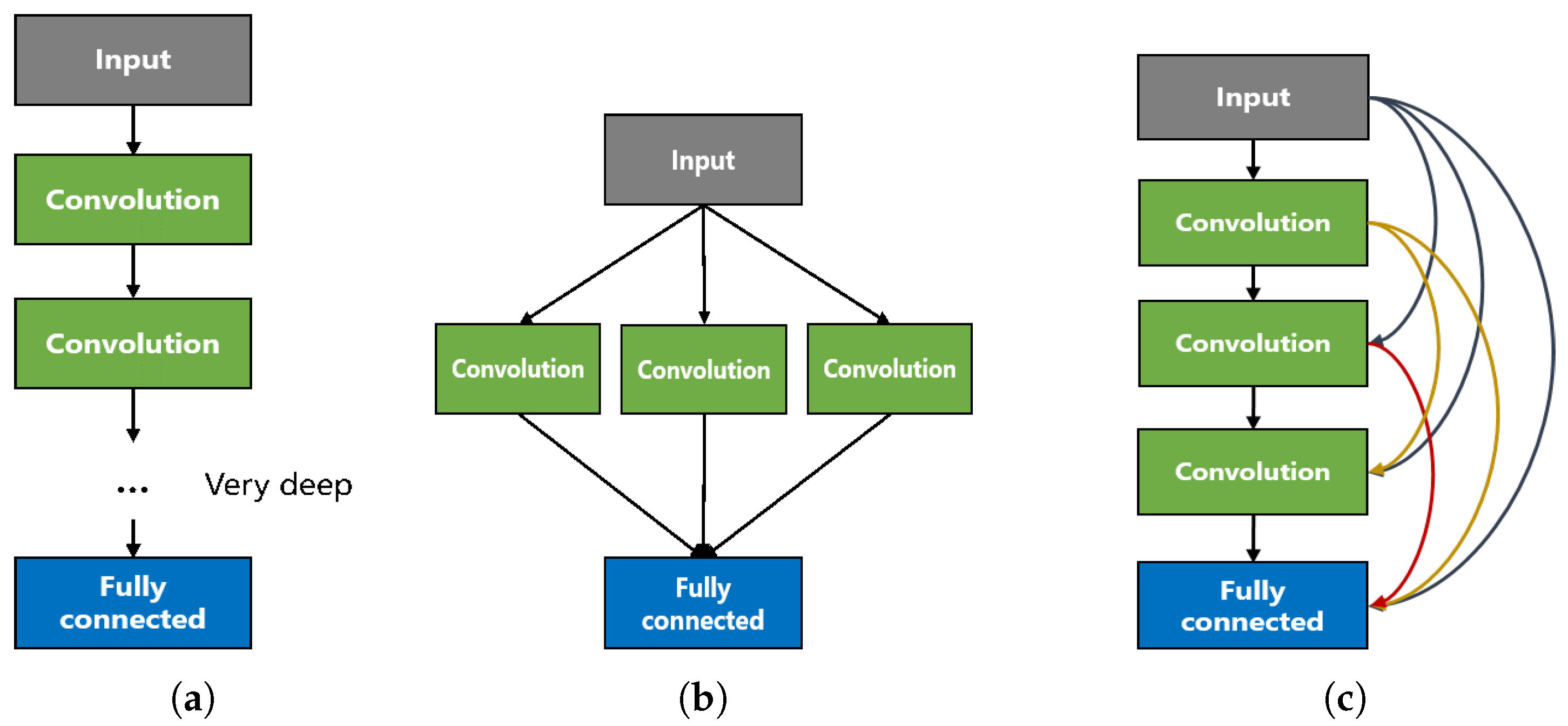
3.1. Architecture of H-ConvNet

The architecture of a typical convolutional neural network (ConvNet) is structured with a series of stages, each of which contains a cascade of layers, such as a convolutional layer, a batch normalization layer, a nonlinearity layer and a scale pooling layer, and with end-to-end feature learning, the data features at multiple levels can be obtained for data categorization [33]. Unlike the commonly very deep design of ConvNet in computer vision, a lightweight 1D ConvNet and 2D ConvNet for the joint exploitation of spectral and context features from MSR image were structured in this study (Figure 3).

3.1.1. 1d Convnet for Spectral Feature Learning

Each pixel in one remote sensing image holds the spectral feature of a specific land cover, and the distinctive feature in each pixel is commonly used for land cover classification. To take full advantage of the spectral information in a remote sensing image, a 1D ConvNet was proposed for deep spectral feature extraction in this study. Unlike the commonly used spectral feature extractors for specific land cover category recognition by predefining the spectral features [35,36], such as NDVI and NDWI, this 1D ConvNet can be fed with raw pixels and automatically exports many distinctive spectral features corresponding to each land cover category, and thus alleviates the need for hand-engineered feature extractors. The most straightforward way to improve the performance of ConvNet is to increase the depth of model size. However, driven by increasing depth, the notorious problem of vanishing/exploding gradients inevitably arises [37,38], which makes model training more difficult. In addition to increasing network depth, increasing model width also contributes to network performance improvement. In this study, considering the relatively limited amount information in a single pixel of multispectral image and inspired by the Inception module of GoogLeNet, a simple 1D ConvNet with a balanced model width and depth was structured for spectral feature learning (Figure 3).

3.1.2. 2d Convnet for Context Feature Learning

To capture the context features of each pixel in a remote sensing image, a 2D ConvNet was designed under the inspiration of dense connectivity, i.e., all layers directly connected to each layer in a feed-forward way [39]; that is, the information moves in only one forward direction, from the input nodes, through the hidden nodes (if any) and to the output nodes. This dense connectivity design has several merits, including alleviating vanishing-gradient problem, strengthening feature propagation and encouraging feature reuse. This 2D ConvNet was designed for a pixelwise land cover classification, and the context feature of per-pixel is characterized by its surrounding patch-based ground area. In particular, context feature-based classification which was performed on the image patches with 5 × 5, 15 × 15 and 25 × 25 pixels was tested, and the optimal patch size of 15 × 15 pixels was finally selected for context feature learning in our study. We structured the 2D ConvNet with three 3 × 3 convolutional layers, and the lth layer receives the feature maps of all preceding layers as input:
x l = H l x 0 , x 1 . . . x l 1
where x 0 , x 1 . . . x l 1 refers to the concatenation of feature maps produced in layers 0, 1,… and l 1 . If each function H l produces k feature maps, then the lth layer will contain k 0 + k × l 1 input feature maps, in which k 0 is the number of image channels in input layer and k is the growth rate of the network. To improve computational efficiency, we introduced a 1 × 1 convolution to reduce the number of input feature maps ahead of each 3 × 3 convolution in network [26]. The consecutive operations of batch normalization (BN) and rectified linear unit (ReLU) were structured to follow all the convolutional layers in our network. Briefly, we can refer to our 2D ConvNet with such a composite layer, i.e., to the Pooling-Conv 1 × 1 -BN-ReLU-Conv 3 × 3 -BN-Relu-Pooling version of H l . In our experiment, we set k = 8 and let each 1 × 1 convolution produce k feature maps. Consequently, the number of input feature maps of 4 , 12 , 20 , 28 can be obtained corresponding to each layer of structured 2D ConvNet.

3.2. Automatic Training Sample Expansion

When applying a machine learning algorithm to remote sensing image classification, some human labeled samples are required for model training. However, the training of a deep learning model commonly requires a large amount of human-labeled samples, and sample labeling is a very laborious process. In this study, to minimize human labor in sample labeling, instead of using the original learning sample for 2D ConvNet training, we proposed an automatic training sample expansion method. The expanded training samples produced by our method were used for full context feature learning. The overview concept and details of training sample expansion regarding the expanded training sample generation are illustrated in Figure 4 and Figure 5, respectively.
The expanded training samples were generated mainly by two steps: (1) the original learning sample-trained 1D ConvNet was used to estimate the category probability of each pixel, and (2) an initial probability threshold was used to determine confidence classification result. To avoid excessive data, which make model training a time-consuming task, the adaptive probability growth and maximum sample size threshold were set to constrain the size of confidence classification result for each category. Specifically, if the resulting confidence classification result exceeds the given maximum value, then the initial probability threshold will be automatically incremented with a fixed probability growth. In this study, we set the parameters of initial probability threshold, adaptive probability growth and maximum sample size with 0.90, 0.005 and 30,000, respectively, and accordingly, the final confidence classification result can be obtained in a fully automatic way. Specifically, the parameters determination details is given in the following Section 5.1.
The confidence classification result obtained using initial probability threshold suffers a sample imbalance problem, which leads to imbalanced feature learning during 2D ConvNet training. We defined R as the sample size ratio between a pair of categories, if the maximum ratio m a x α , b c a t e g o r i e s R α , b of the category pairs is larger than a predefined maximum ratio r, which is set to 3 in our study, the sample size is regarded as unbalanced, and then further sample equalization is. Furthermore, we introduced an exponential transformation method for sample equalization. Specifically, with the given maximum ratio r, the exponential transformation parameters can be calculated according to m a x α , b c a t e g o r i e s R a , b s = r ; and then, a relatively reasonable proportion R can be obtained through exponential transformation R e q = R s . The redundant pixels of confidence classification result were removed by a random spatial approach, and the remaining classified pixels were regarded as final expanded training samples. Generally, sample equalization is crucial for subsequent 2D ConvNet-based classification; however, if the maximum ratio parameter falls into a reasonable scope of 1–4, then the maximum ratio parameter only slightly affects classification accuracy.

3.3. Model Training and Classification

3.3.1. Model Training

The power of ConvNet depends on the weights involved in convolutional filters used to produce the distinctive feature maps through feed-forward propagation. Therefore, it is very important to obtain optimal convolutional filters with respect to each layer of network. The gradient back propagation algorithm, a core fundamental component of neural networks, can be applied for parameters updating by repeatedly propagating gradients through all modules, starting from the output at top (where the network produces its prediction) to bottom (where the original input is fed). Before the parameters were updated along with proposed H-ConvNet training, the model parameters were initialized using a normal distribution function with a certain mean of 0 and a standard deviation of 0.01 in this study.
To obtain gradient, an objective function should be predefined for network, and we used cross entropy loss as objective function in this study. Additionally, considering that overfitting weakens generalization ability, we introduced L2 regularization to mitigate the overfitting problem of proposed model. Thus, the objective function containing a cross entropy loss, which measures the difference between two probability distributions [40], and a regularization term is given as follow:
J y , p , w = 1 n i = 1 k y i log p i + 1 y i log 1 p i + λ 2 w 2 2
where J y , p , w is objective function; y, p and w denote target class probability, predicted class probability and network weights, respectively; k is the number of categories in classification; and λ is L2 regularization parameter, which is used to prevent model overfitting by controlling L2 regularization intensity. To obtain an optimal regularization parameter, a simple grid search was performed using a holdout of 20% of training data for validation. As we employed a mini-batch update strategy, the cost was computed based on a mini batch of inputs. n denotes the size of mini batch.
The proposed H-ConvNet consists of one 1D ConvNet and one 2D ConvNet, and the training process of our H-ConvNet contains three steps: (1) the 1D ConvNet is trained with a limited number of training samples; (2) a training sample expansion is performed using pretrained 1D ConvNet, and (3) the expanded training samples are used for 2D ConvNet training. For optimization, Adam (Kingma and Ba, 2014) with momentum parameters β 1 = 0 . 5 , β 2 = 0 . 999 is applied, the learning rate and mini batch size are set to 0.002 and 8 for 1D ConvNet, and 0.001 and 8 for 2D ConvNet trainings, and the training procedures stop after no improvement in the cost function is observed after 100 epochs and 500 epochs during 1D ConvNet and 2D ConvNet trainings, respectively.

3.3.2. Land Cover Category Determination

We applied the original and expanded training samples for the training of 1D ConvNets and 2D ConvNet, respectively. Thus, for any input pixel location of image, both spectral features and context features can be obtained through the implementation of well-trained ConvNets. The land cover category of each image pixel was determined according to the more prominent features that is quantified by feature-based classification probability (Equation (3)):
c i = a r g m a x k c l a s s e s p k i s p e c t r a l , p k i s c e n e
where i is input image pixel, c is corresponding classification result, and p k i s p e c t r a l and p k i s c e n e represent spectral feature-based and context feature-based classification probabilities, respectively. With the collaboration of obtained spectral and context features, a pixelwise urban land cover mapping was performed on remote sensing image.

3.4. Methods Comparison

The performance of H-ConvNets was quantitatively evaluated by comparing with existing classification methods, including support vector machine (SVM), object-based image analysis (OBIA), Markov random field model (MRF) and newly proposed patch-based CNN system [17]. The patch-based CNNs was implemented strictly accoeding to Sharma et al. [17], and the detailed implementations of other three methods are given as follows:
SVM: The radial basis function (RBF) kernel was adopted. As the two parameters of penalty value C and kernel width σ should be configured for SVM implementation, we searched the optimal parameters within the parameter space of 8 , 16 , 32 , 64 , 128 , 256 , 512 , 1024 and 0.005 , 0.01 , 0.05 , 0.1 , 0.5 , 1 corresponding to C and σ parameters, respectively, through a grid-search method with 5-fold cross validation.
OBIA: A multiresolution segmentation algorithm was initially implemented to segment objects throughout image. Three key parameters, namely, scale, color and compactness, were required in image segmentation, and for each of the parameter values, the scale parameter varied the most, as it was the most influential parameter [41]. In the comparison experiments, the parameters of color and compactness were constantly set to 0.9 and 0.5, respectively, and the optimal scale parameter was determined within the parameter space of 50 , 60 , 70 , 80 , 90 , 100 by using a trial-and-error method. The trial-and-error method is laborious and thus time consuming; however, for a convincing comparative test, we expect high accuracy rather than higher efficiency in OBIA implementation. Therefore, although some semiautomatic and automatic methods have been proposed for scale parameter determination [42,43,44,45], the trial-and-error method was still adopted in our study. On the basis of generated objects, a range of features, including mean value, standard deviation and gray-level cooccurrence matrix, were fed into a parameterized SVM for object-based image classification.
MRF: A Markov random fields (MRF), which is used to model contextual correlation among image pixels in terms of the conditional prior probabilities of individual pixels given by their neighboring pixels, and thus the spatial dependencies within a pixel neighborhood can be used to support the classification of central pixel [46,47]. For the implementation of MRF method, the conditional prior probability was calculated using a probabilistic SVM method [48], and the spatial context was incorporated by a predefined four-neighborhood system according to SVM classification result. The optimal smoothness parameter β was determined within the parameter space of 0 . 5 , 1 , 2 , 4 , 8 , 16 , 32 , and the α -expansion graph-cut-based algorithm was employed to optimize the MRF energy function with iterations.

4. Results

4.1. H-ConvNet, 1D ConvNet and 2D ConvNet

With the implementation of H-ConvNet, an urban land cover map, which consists of four biophysical land cover categories of water, vegetation, soil and impervious surfaces, was produced (Figure 6). To illustrate the efficiency of feature cooperation in mapping urban land cover, we conducted a comparative analysis among the urban land cover maps derived by 1D ConvNet, 2D ConvNet and H-ConvNet. The comparative analysis among the urban land cover maps derived by 1D ConvNet, 2D ConvNet and H-ConvNet are shown in Figure 6. The spectral feature-based 1D ConvNet could capture more detailed geospatial variations in urban region, while it inevitably suffered pixel-level misclassification, particularly for the distinction of impervious and soil surfaces (Figure 6c,g,k). Meanwhile, the 1D ConvNet model demonstrated a serious spatial discontinuity in urban landscape mapping. The context feature-based 2D ConvNet does the exact opposite by assigning a land cover category of a given context to central pixel. The 2D ConvNet produced a space-continuous landscape map while suffering from misclassifications when encountering a heterogeneous urban environment (Figure 6d,h,l). The urban maps of Figure 6b,f,j show that the H-ConvNet overcomes the shortcomings of respective spectral feature-based 1D ConvNet and context feature-based 2D ConvNet, and thus achieve the best performance in urban land cover mapping.

4.2. H-Convnet Validation and Comparison

4.2.1. Classification in Terms of the Biophysical Composition and Land Use

The proposed H-ConvNet model is evaluated by mapping the urban land cover in terms of biophysical compositions and land use. By comparing the corrected pixels of each classification map to the reference map, the proposed H-ConvNet achieved the highest overall accuracy of 87.15% in the 4-class urban mapping (Figure 7), followed by the Patch-based CNNs (82.87%), MRF (81.36%), SVM (81.10%) and OBIA (81.92%). This algorithm achieved the highest overall accuracy of 81.04% in the 6-class urban mapping, followed by the Patch-based CNNs (79.85%), MRF (77.62%), OBIA (77.61%) and SVM (76.94%) (Figure 7). The producer’s accuracy [49], which is calculated through a division operation of the number of accurately classified reference samples and the total number of reference samples for that class, is used for a further accuracy analysis by the form of confusion matrices. As illustrated in Figure 8 and Figure 9, the four-class land cover mapping experiences serious confusion between the soil and impervious surface, while the six-class land cover mapping suffers observable confusion among the urban living area, urban industrial area and bare land. In general, through a comparison of the methods, the H-ConvNet achieved the best performance in land cover mapping with relatively less confusion in both the four-class and six-class land cover classifications.

4.2.2. Urban Land Cover Mapping with Additional Test Regions

To further validate the performance and superiority of the proposed H-ConvNet, in our study, we selected five additional test regions corresponding to the cities of London, New York, Paris, Seoul and Tokyo (Figure 10). These five urban regions are all with high surface heterogeneity and with different urban landscapes, which is suit for the testing of the proposed classification method. With the acquired Sentinel-2 images, a series of preprocessing methods, such as atmospheric correction, and cloud mask, are carried out first, and then, the pixel-based training and validation samples are collected using a stratified random sampling strategy which is mentioned in Section 2.2. Specifically, for the five study areas of London, New York, Paris, Seoul and Tokyo, the numbers of training pixels are 2780, 1221, 829, 657 and 1151, and the numbers of testing pixels are 17,411, 27,470, 17,816, 12,848 and 17,141, respectively. The proposed H-ConvNet and comparison methods are applied to six-class urban land cover mapping in all the test regions (Figure 11). According to the quantitative accuracy assessment (Figure 12), the proposed H-ConvNet performs the best in all test regions of London, New York, Paris, Seoul and Tokyo that is, the proposed H-ConvNet achieved the highest overall accuracies of 77.21%, 90.14%, 87.16%, 89.05% and 87.65%, respectively (Figure 12). The accuracies derived by the comparison methods vary in urban landscapes; for example, the OBIA achieved the second highest overall accuracy in the London and New York test regions, while it achieves the second lowest overall accuracy in the Seoul test region. The MRF model achieved the second highest overall accuracy in the Paris and Seoul test regions, while it achieved the lowest accuracy in the London test region. The SVM performs better in the Seoul and Tokyo test regions, while it loses much accuracy in the New York and Paris test regions. Generally, the methods commonly have their specific applicability and perform well when the algorithms fit the test urban landscape. Our proposed method achieved the highest accuracy in all the selected urban regions, further demonstrating the superiority of this method in terms of both high accuracy and robustness compared to the existing classification methods.

5. Analysis and Discussion

5.1. The Improvement in the Convnet with the Expanded Sample Training

To fully learn the context features of land cover categories, we exploit a training sample expanding strategy that aims to acquire enough training samples for structured 2D ConvNet training. Through an example expansion process, the quantity of the training samples are expanded to nearly 100-fold for the study region and provide more context information for 2D context feature learning (Figure 13). In this section, we accessed the effect of an expanded training sample on urban land cover mapping in practice. As Figure 14 shows, when compared to the original training sample-trained 2D ConvNet, the expanded learning sample-trained model achieves an improved urban mapping with a higher 7.81% of the average overall accuracy. As the result shows, a large number of training samples benefit the context features learning by using the 2D ConvNet, and the proposed training sample expanding strategy is demonstrated to be effective. Moreover, when the new H-ConvNet is structured by the expanded sample-trained 2D ConvNet, the urban land cover mapping enhanced to a certain in comparison with the original sample-trained H-ConvNet (Figure 14).
The automatic sample expanding method requires four predefined parameters, and therefore, we can further evaluate the sensitivity of the parameters in this section. We carried out experiments by setting the parameters to different values. As shown in the experimental results in Table 1 and Table 2, when the parameters fall into reasonable scopes, these parameters slightly affect the final classification result. Specifically, we think the initial probability threshold is larger than 0.85, the adaptive probability growth lies within the approximate range 0.001–0.005, the maximum sample lies within the approximate range 20,000–40,000, and the maximum ratio lies within the approximate range 1–4. Accordingly, in our study, we set the four parameters to 0.90, 0.005, 30,000, and 3.

5.2. Applicability of Spectral/Context Feature-Based Urban Mapping

The proposed H-ConvNet improves the urban land cover mapping through an effective collaboration of the spectral feature-oriented 1D ConvNet and context feature-oriented 2D ConvNet. Specifically, the 2D ConvNet is trained using an expanded training sample, which is obtained through a combination with the spectral feature-based classification result. Generally, three solutions can be obtained for land cover mapping with different application requirements in our study: (1) spectral feature-based 1D ConvNet, (2) context feature-based 2D ConvNet, and (3) spectral and context feature-based H-ConvNet. We test the performance of the three solutions by considering the mapping accuracy, model stability, operation efficiency and landscape mapping quality by using the indictors of the respective average overall accuracy, accuracy standard deviation, time consuming and patch density. As Table 3 illustrates, the structured ConvNets achieved the highest overall accuracy with a decreasing order of H-ConvNet, 2D ConvNet and 1D ConvNet. However, as demonstrated by the standard deviation of the accuracies, the 1D ConvNet model is the most stable model, followed by the H-ConvNet and 2D ConvNet. Additionally, we can see the significant difference of the mapping quality derived from different mapping solutions (Figure 6); that is, the 2D ConvNet-based urban land cover mapping model achieves a low patch density and thus shows a high landscape continuity of the obtained land cover map. However the spectral-based 1D ConvNet experiences much salt-pepper noise during image classification, and thus, a high landscape fragmentation of the derived land cover map occurs. By taking both the mapping accuracy and visualization mapping quality into account, the H-ConvNet performs the best due to an effective collaboration of spectral and context features.
Nevertheless, although the proposed H-ConvNet performs the best in terms of the classification accuracy, the H-ConvNet consists of one 1D ConvNet and one 2D ConvNet, and thus the implementation of H-ConvNet is relatively time-consuming using a computer with a CPU configuration. As Table 3 illustrates, the H-ConvNet costs ten times longer than the 1D ConvNet in land cover/land use classification. Taken together, the structured ConvNets have their respective applicability and can be used to for different applications. The H-ConvNet, which has advantages with high accuracy and high model stability, is the most preferred solution in urban land cover mapping. Moreover, the structured 1D ConvNet is also a good option when time efficiency is required, and the 2D ConvNet is applicable when the visualization mapping quality is regarded as the most important factor.

5.3. Comparison to Semantic Segmentation Models and Further Research

Semantic segmentation involves classifying each pixel in an image into a class in the field of computer vision [50]. This method has also shown great potential in pixelwise satellite images classification. Generally, common semantic segmentation models are designed with a 2-D encoder-decoder structure, and state-of-the-art models are commonly structured with very deep layers to guarantee accuracy. Compared to semantic segmentation (Table 4), the newly proposed H-ConvNet is designed with a hybrid 3-D structure that corresponds to 3-D information analysis for multispectral satellite image. H-ConvNet is also designed as a lightweight network that provides rapid model implementation under limited computing resources condition (e.g., CPU configuration only). In addition, the training conditions in terms of sample quantity and sample design for semantic segmentation models and H-ConvNet are also different. Unlike in the semantic segmentation models, which require large numbers of human-annotated training samples for feature learning, thereby limiting the intelligent design of these methods, H-ConvNet can perform well when only a limited number of human-annotated training samples is provided. From the perspective of sample design, H-ConvNet requires pixel-based sample inputs, and semantic segmentation models require patch-based sample inputs. Current studies have explored many state-of-the-art semantic segmentation models for the image classification in the field of computer vision [50,51,52]; however, there are still many issues that prevent the directly transfer use of the existing models from computer vision to remote sensing. First of all, the high-quality datasets for feature learning with respect to different remote sensing applications are lacking. Second, common deep learning methods require large amounts of training data and high performance computing resource, thereby limits the widespread application of the deep learning method. Therefore, in the further study, more high-quality datasets are needed to be developed for the state-of-the-art deep learning model training. On the other hand, on the premise of this study, the semi-supervised or weakly supervised deep learning model with a lightweight network structure is also required to be further explored.

6. Conclusions

It is difficult to capture the distinctive features of land cover categories in heterogeneous urban environments, which makes it challenging to map the urban land cover with high precision. The advanced deep ConvNets have brought breakthroughs in the field of computer vision [33]; however, due to the image data gap between the domains of remote sensing and computer vision, it is still challenging to directly and efficiently apply state-of-the-art ConvNets for remote sensing applications. When structuring a ConvNet for remote sensing image classification, the difference in the image modality between remote sensing and computer vision should be considered. Specifically, (1) the remote sensing images are acquired from a satellite view and with significantly changeable spatial resolutions (e.g., approximately 1–1000 m ), whereas the images in computer vision are always acquired from a human view and with high spatial resolution. (2) Rather than a color image, which is commonly composed of three-color channels, the remote sensing image contains several (e.g., 4–10) or even hundreds of color channels corresponding to the multispectral and hyperspectral image, respectively. (3) In computer vision, massive data sets corresponding to specific applications have been built for ConvNet training; however, very few training data sets are built for feature learning from remote sensing image. Therefore, the model training strategy that is based on a small amount of training samples is still adopted for ConvNet training and thus results in the low efficiency and universality of the trained ConvNets in remote sensing image classification. Notably, the semantic segmentation method in computer vision can also be used for per-pixel remote sensing image classification; however, semantic segmentation requires patch-based labeled data for model training, which makes the implementation of image classification different from our proposed method. Therefore, the semantic segmentation method is not compared in this study.
Many researchers have explored the application potential of ConvNet in high-resolution remotely sensed image processing; however, few ConvNet application studies haves been tailored for moderate-resolution remote sensing image. In this study, we proposed a new lightweight H-ConvNet for the enhancement of urban land cover mapping using Sentinel-2 moderate-resolution image. Through experimental testing, the H-ConvNet achieved a significant improvement compared with the existing classification methods, including SVM, OBIA, MRF model and patch-based CNNs. In general, the main contributions of this paper can be summarized as follows: (1) with the inspiration of the advanced deep learning technique, we designed a new H-ConvNet that is particularly applicable for heterogeneous urban land cover mapping based on moderate-resolution image. Due to the superiority of the proposed H-ConvNet and the large amount of moderate-resolution data reserves, this H-ConvNet demonstrates great potential with respect to large-scale land investigations. (2) The structured spectral-based 1D ConvNet and context-based 2D ConvNet can also be used for land cover mapping alone in some cases. To fully learn the context features via a structured 2D ConvNet, a training sample expanding strategy is proposed and is shown to be effective in our study.

Author Contributions

Conceptualization, X.L. and X.T.; methodology, X.L.; validation, X.L. and Z.H.; formal analysis, X.L. and G.W.; writing—original draft preparation, X.L.; writing—review and editing, Z.H. and G.W.; supervision, X.T. and G.W. All authors have read and agreed to the published version of the manuscript.

Acknowledgments

This work was jointly supported by the National Key R&D Program of China (No.2017YFC0506200), by the National Natural Science Foundation of China (NSFC) (No. 41871227, No.41631178), by the Natural Science Foundation of Guangdong (No.2020A1515010678), and by the Basic Research Program of Shenzhen (No.JCYJ20190808122405692). And the European Space Agency provided Sentinel-2 image data.

Conflicts of Interest

The authors declare no conflict of interest.

References

  1. Turner, B.L.; Lambin, E.F.; Reenberg, A. The emergence of land change science for global environmental change and sustainability. Proc. Natl. Acad. Sci. USA 2007, 104, 20666–20671. [Google Scholar] [CrossRef] [PubMed] [Green Version]
  2. Yu, W.; Zhou, W.; Qian, Y.; Yan, J. A new approach for land cover classification and change analysis: Integrating backdating and an object-based method. Remote Sens. Environ. 2016, 177, 37–47. [Google Scholar] [CrossRef]
  3. Zhou, W.; Huang, G.; Troy, A.; Cadenasso, M. Object-based land cover classification of shaded areas in high spatial resolution imagery of urban areas: A comparison study. Remote Sens. Environ. 2009, 113, 1769–1777. [Google Scholar] [CrossRef]
  4. Gong, P.; Wang, J.; Yu, L.; Zhao, Y.; Zhao, Y.; Liang, L.; Niu, Z.; Huang, X.; Fu, H.; Liu, S. Finer resolution observation and monitoring of global land cover: First mapping results with Landsat TM and ETM+ data. Int. J. Remote Sens. 2013, 34, 2607–2654. [Google Scholar] [CrossRef] [Green Version]
  5. Momeni, R.; Aplin, P.; Boyd, D.S. Mapping complex urban land cover from spaceborne imagery: The influence of spatial resolution, spectral band set and classification approach. Remote Sens. 2016, 8, 88. [Google Scholar] [CrossRef] [Green Version]
  6. Lu, D.; Weng, Q. A survey of image classification methods and techniques for improving classification performance. Int. J. Remote Sens. 2007, 28, 823–870. [Google Scholar] [CrossRef]
  7. Huang, K.Y. A synergistic automatic clustering technique (SYNERACT) for multispectral image analysis. Photogramm. Eng. Remote. Sens. 2002, 68, 33–40. [Google Scholar]
  8. Strahler, A.H. The use of prior probabilities in maximum likelihood classification of remotely sensed data. Remote Sens. Environ. 1980, 10, 135–163. [Google Scholar] [CrossRef]
  9. Mas, J.F.; Flores, J.J. The application of artificial neural networks to the analysis of remotely sensed data. Int. J. Remote Sens. 2008, 29, 617–663. [Google Scholar] [CrossRef]
  10. Pal, M. Random forest classifier for remote sensing classification. Int. J. Remote Sens. 2005, 26, 217–222. [Google Scholar] [CrossRef]
  11. Mountrakis, G.; Im, J.; Ogole, C. Support vector machines in remote sensing: A review. ISPRS J. Photogramm. Remote Sens. 2011, 66, 247–259. [Google Scholar] [CrossRef]
  12. Kraaijenbrink, P.; Shea, J.; Pellicciotti, F.; De Jong, S.; Immerzeel, W. Object-based analysis of unmanned aerial vehicle imagery to map and characterise surface features on a debris-covered glacier. Remote Sens. Environ. 2016, 186, 581–595. [Google Scholar] [CrossRef]
  13. Chen, Y.; Ge, Y.; Heuvelink, G.B.; An, R.; Chen, Y. Object-based superresolution land-cover mapping from remotely sensed imagery. IEEE Trans. Geosci. Remote Sens. 2018, 56, 328–340. [Google Scholar] [CrossRef]
  14. Li, M.; Ma, L.; Blaschke, T.; Cheng, L.; Tiede, D. A systematic comparison of different object-based classification techniques using high spatial resolution imagery in agricultural environments. Int. J. Appl. Earth Obs. Geoinf. 2016, 49, 87–98. [Google Scholar] [CrossRef]
  15. Xu, L.; Zhang, H.; Zhao, M.; Chu, D.; Li, Y. Integrating spectral and spatial features for hyperspectral image classification using low-rank representation. In Proceedings of the 2017 IEEE International Conference on Industrial Technology (ICIT), Toronto, ON, Canada, 22–25 March 2017; IEEE: Piscataway, NJ, USA, 2017; pp. 1024–1029. [Google Scholar]
  16. Myint, S.W.; Gober, P.; Brazel, A.; Grossman-Clarke, S.; Weng, Q. Per-pixel vs. object-based classification of urban land cover extraction using high spatial resolution imagery. Remote Sens. Environ. 2011, 115, 1145–1161. [Google Scholar] [CrossRef]
  17. Sharma, A.; Liu, X.; Yang, X.; Shi, D. A patch-based convolutional neural network for remote sensing image classification. Neural Netw. 2017, 95, 19–28. [Google Scholar] [CrossRef]
  18. Dalal, N.; Triggs, B. Histograms of oriented gradients for human detection. In Proceedings of the 2005 IEEE Computer Society Conference on Computer Vision and Pattern Recognition (CVPR’05), San Diego, CA, USA, 20–26 June 2005; IEEE: Piscataway, NJ, USA, 2005; Volume 1, pp. 886–893. [Google Scholar]
  19. Tsai, C.F. Bag-of-words representation in image annotation: A review. ISRN Artif. Intell. 2012, 2012. [Google Scholar] [CrossRef]
  20. Nogueira, K.; Penatti, O.A.; Dos Santos, J.A. Towards better exploiting convolutional neural networks for remote sensing scene classification. Pattern Recognit. 2017, 61, 539–556. [Google Scholar] [CrossRef] [Green Version]
  21. Huang, B.; Zhao, B.; Song, Y. Urban land-use mapping using a deep convolutional neural network with high spatial resolution multispectral remote sensing imagery. Remote Sens. Environ. 2018, 214, 73–86. [Google Scholar] [CrossRef]
  22. Zhu, X.X.; Tuia, D.; Mou, L.; Xia, G.S.; Zhang, L.; Xu, F.; Fraundorfer, F. Deep learning in remote sensing: A comprehensive review and list of resources. IEEE Geosci. Remote Sens. Mag. 2017, 5, 8–36. [Google Scholar] [CrossRef] [Green Version]
  23. He, K.; Zhang, X.; Ren, S.; Sun, J. Deep residual learning for image recognition. In Proceedings of the IEEE Conference on Computer Vision and Pattern Recognition (CVPR), Las Vegas, NV, USA, 27–30 June 2016; pp. 770–778. [Google Scholar]
  24. Krizhevsky, A.; Sutskever, I.; Hinton, G.E. Imagenet classification with deep convolutional neural networks. In Advances in Neural Information Processing Systems; MIT: Cambridge, MA, USA, 2012; pp. 1097–1105. [Google Scholar]
  25. Simonyan, K.; Zisserman, A. Very deep convolutional networks for large-scale image recognition. arXiv 2014, arXiv:1409.1556. [Google Scholar]
  26. Szegedy, C.; Liu, W.; Jia, Y.; Sermanet, P.; Reed, S.; Anguelov, D.; Erhan, D.; Vanhoucke, V.; Rabinovich, A. Going deeper with convolutions. In Proceedings of the IEEE Conference on Computer Vision and Pattern Recognition (CVPR), Boston, MA, USA, 7–12 June 2015; pp. 1–9. [Google Scholar]
  27. Xu, X.; Li, W.; Ran, Q.; Du, Q.; Gao, L.; Zhang, B. Multisource remote sensing data classification based on convolutional neural network. IEEE Trans. Geosci. Remote Sens. 2017, 56, 937–949. [Google Scholar] [CrossRef]
  28. Zhang, C.; Sargent, I.; Pan, X.; Li, H.; Gardiner, A.; Hare, J.; Atkinson, P.M. An object-based convolutional neural network (OCNN) for urban land use classification. Remote Sens. Environ. 2018, 216, 57–70. [Google Scholar] [CrossRef] [Green Version]
  29. Cheng, G.; Li, Z.; Han, J.; Yao, X.; Guo, L. Exploring hierarchical convolutional features for hyperspectral image classification. IEEE Trans. Geosci. Remote Sens. 2018, 56, 6712–6722. [Google Scholar] [CrossRef]
  30. Zhou, P.; Han, J.; Cheng, G.; Zhang, B. Learning compact and discriminative stacked autoencoder for hyperspectral image classification. IEEE Trans. Geosci. Remote Sens. 2019, 57, 4823–4833. [Google Scholar] [CrossRef]
  31. Lin, L.; Chen, C.; Xu, T. Spatial-spectral hyperspectral image classification based on information measurement and CNN. Eurasip J. Wirel. Commun. Netw. 2020, 2020, 1–16. [Google Scholar] [CrossRef]
  32. Li, S.; Song, W.; Fang, L.; Chen, Y.; Ghamisi, P.; Benediktsson, J.A. Deep learning for hyperspectral image classification: An overview. IEEE Trans. Geosci. Remote Sens. 2019, 57, 6690–6709. [Google Scholar] [CrossRef] [Green Version]
  33. LeCun, Y.; Bengio, Y.; Hinton, G. Deep learning. Nature 2015, 521, 436–444. [Google Scholar] [CrossRef]
  34. Drusch, M.; Del Bello, U.; Carlier, S.; Colin, O.; Fernandez, V.; Gascon, F.; Hoersch, B.; Isola, C.; Laberinti, P.; Martimort, P. Sentinel-2: ESA’s optical high-resolution mission for GMES operational services. Remote Sens. Environ. 2012, 120, 25–36. [Google Scholar] [CrossRef]
  35. McFeeters, S.K. The use of the Normalized Difference Water Index (NDWI) in the delineation of open water features. Int. J. Remote Sens. 1996, 17, 1425–1432. [Google Scholar] [CrossRef]
  36. Rouse, J.; Haas, R.; Schell, J.; Deering, D. Monitoring vegetation systems in the Great Plains with ERTS. NASA Spec. Publ. 1974, 351, 309. [Google Scholar]
  37. Bengio, Y.; Simard, P.; Frasconi, P. Learning long-term dependencies with gradient descent is difficult. IEEE Trans. Neural Netw. 1994, 5, 157–166. [Google Scholar] [CrossRef]
  38. Glorot, X.; Bengio, Y. Understanding the difficulty of training deep feedforward neural networks. In Proceedings of the Thirteenth International Conference on Artificial Intelligence and Statistics, Sardinia, Italy, 13–15 May 2010; pp. 249–256. [Google Scholar]
  39. Huang, G.; Liu, Z.; Van Der Maaten, L.; Weinberger, K.Q. Densely connected convolutional networks. In Proceedings of the IEEE Conference on Computer Vision and Pattern Recognition (CVPR), Honolulu, HI, USA, 21–26 July 2017; pp. 4700–4708. [Google Scholar]
  40. Bruch, S.; Wang, X.; Bendersky, M.; Najork, M. An analysis of the softmax cross entropy loss for learning-to-rank with binary relevance. In Proceedings of the 2019 ACM SIGIR International Conference on Theory of Information Retrieval, Santa Clara, CA, USA, 2–5 October 2019; pp. 75–78. [Google Scholar]
  41. Luo, H.; Wang, L.; Shao, Z.; Li, D. Development of a multi-scale object-based shadow detection method for high spatial resolution image. Remote Sens. Lett. 2015, 6, 59–68. [Google Scholar] [CrossRef]
  42. Zhang, H.; Fritts, J.E.; Goldman, S.A. Image segmentation evaluation: A survey of unsupervised methods. Comput. Vis. Image Underst. 2008, 110, 260–280. [Google Scholar] [CrossRef] [Green Version]
  43. Kim, M.; Madden, M.; Warner, T. Estimation of optimal image object size for the segmentation of forest stands with multispectral IKONOS imagery. In Object-Based Image Analysis; Springer: Berlin/Heidelberg, Germany, 2008; pp. 291–307. [Google Scholar]
  44. Drăguţ, L.; Csillik, O.; Eisank, C.; Tiede, D. Automated parameterisation for multi-scale image segmentation on multiple layers. ISPRS J. Photogramm. Remote Sens. 2014, 88, 119–127. [Google Scholar] [CrossRef] [PubMed] [Green Version]
  45. Johnson, B.; Xie, Z. Unsupervised image segmentation evaluation and refinement using a multi-scale approach. ISPRS J. Photogramm. Remote Sens. 2011, 66, 473–483. [Google Scholar] [CrossRef]
  46. Wang, L.; Liu, J. Texture classification using multiresolution Markov random field models. Pattern Recognit. Lett. 1999, 20, 171–182. [Google Scholar] [CrossRef]
  47. Xia, J.; Chanussot, J.; Du, P.; He, X. Spectral–spatial classification for hyperspectral data using rotation forests with local feature extraction and Markov random fields. IEEE Trans. Geosci. Remote Sens. 2014, 53, 2532–2546. [Google Scholar] [CrossRef]
  48. Platt, J. Probabilistic outputs for support vector machines and comparisons to regularized likelihood methods. Adv. Large Margin Classif. 1999, 10, 61–74. [Google Scholar]
  49. Congalton, R.G.; Green, K. Assessing the Accuracy of Remotely Sensed Data: Principles and Practices; CRC Press: Boca Raton, FL, USA, 2019. [Google Scholar]
  50. Long, J.; Shelhamer, E.; Darrell, T. Fully convolutional networks for semantic segmentation. In Proceedings of the IEEE Conference on Computer Vision and Pattern Recognition (CVPR), Boston, MA, USA, 7–12 June 2015; pp. 3431–3440. [Google Scholar]
  51. Chen, L.C.; Zhu, Y.; Papandreou, G.; Schroff, F.; Adam, H. Encoder-decoder with atrous separable convolution for semantic image segmentation. In Proceedings of the European Conference on Computer Vision (ECCV), Munich, Germany, 8–14 September 2018; pp. 801–818. [Google Scholar]
  52. Liu, C.; Chen, L.C.; Schroff, F.; Adam, H.; Hua, W.; Yuille, A.L.; Li, F.-F. Auto-deeplab: Hierarchical neural architecture search for semantic image segmentation. In Proceedings of the IEEE Conference on Computer Vision and Pattern Recognition (CVPR), Long Beach, CA, USA, 16–20 June 2019; pp. 82–92. [Google Scholar]
Figure 1. A true-color composite Sentinel-2 image showing the heterogeneous urban region in our study.
Remotesensing 12 02292 g001
Figure 2. Workflow of spectral-context feature joint urban land cover mapping using proposed H-ConvNet. The colors in class prediction represent different land cover/land use classes.
Remotesensing 12 02292 g002
Figure 3. Illustration of the lightweight structure designs of our study: (a) Commonly very deep ConvNet; (b) lightweight 1D ConvNe; and (c) lightweight 2D ConvNet design.
Remotesensing 12 02292 g003
Figure 4. Overview concept of training sample expansion method.
Remotesensing 12 02292 g004
Figure 5. Automatic training sample expansion method. The colors of rectangles and lines represent different land cover/land use classes.
Remotesensing 12 02292 g005
Figure 6. Urban land cover maps derived by H-ConvNet, 1D ConvNet and 2D ConvNet: (a) Scenario A; (b) result of H-ConvNet for Scenario A; (c) result of 1D ConvNet for Scenario A; (d) result of 2D ConvNet for Scenario A; (e) Scenario B; (f) result of H-ConvNet for Scenario B; (g) result of 1D ConvNet for Scenario B; (h) result of 2D ConvNet for Scenario B; (i) result of Scenario C; (j) result of H-ConvNet for Scenario C; (k) result of 1D ConvNet for Scenario C; (l) result of 2D ConvNet for Scenario C.
Remotesensing 12 02292 g006aRemotesensing 12 02292 g006b
Figure 7. Accuracy comparisons of the urban maps produced by the patch-based CNNs, SVM, RF, NN and the new proposed H-ConvNet.
Remotesensing 12 02292 g007
Figure 8. Urban land cover maps derived by H-ConvNet, 1D ConvNet and 2D ConvNet: (a) confusion matrix derived by H-ConvNet; (b) confusion matrix derived by SVM; (c) confusion matrix derived by OBIA; (d) confusion matrix derived by MRF; (e) confusion matrix derived by Patch-based CNNs. The colors from white to black represent the values from 0 to 1.
Remotesensing 12 02292 g008
Figure 9. Urban land cover maps derived by H-ConvNet, 1D ConvNet and 2D ConvNet: (a) confusion matrix derived by H-ConvNet; (b) confusion matrix derived by SVM; (c) confusion matrix derived by OBIA; (d) confusion matrix derived by MRF; (e) confusion matrix derived by Patch-based CNNs. The colors from white to black represent the values from 0 to 1.
Remotesensing 12 02292 g009aRemotesensing 12 02292 g009b
Figure 10. The additional test regions displayed by true-color composite Sentinel-2 image. The regions marked in yellow and red represent the distributions of the training and testing samples, respectively: (a) distribution of the text areas; (b) London; (c) New York; (d) Paris; (e) Seoul; (f) Tokyo.
Remotesensing 12 02292 g010
Figure 11. Land cover maps derived by the proposed H-ConvNets: (a) result of London; (b) result of New York; (c) result of Paris; (d) result of Seoul; (e) result of Tokyo.
Remotesensing 12 02292 g011
Figure 12. Method comparisons among the five additional test regions.
Remotesensing 12 02292 g012
Figure 13. The distribution of the original and expanded training samples: (a) original training samples; (b) Expanded training samples; (c) Scenario A; (d) Scenario B; (e) Scenario C.
Remotesensing 12 02292 g013
Figure 14. Comparisons of the overall classification accuracy of the 2D ConvNet and H-ConvNet model those to be trained by the original and expanded training sample, respectively. The results are derived by repeated experiments, and exact 95% confidence intervals plotted.
Remotesensing 12 02292 g014
Table 1. Parameter setting and the corresponding results, including running time during the training sample expansion and the overall accuracy of the 2D ConvNet.
ParametersRunning TimeOverall Accuracy
Initial
Probability
Threshold
Adaptive
Probability
Growth
Maximum
Number
Initial
Sample-Trained
Expanded
Sample-Trained
Group 10.950.00130,0007 s70.96%77.58%
Group 20.90.000520,00086 s 77.29%
Group 30.850.0240,00040 s 78.59%
Table 2. The maximum ratio parameters setting and the corresponding results, including the ratios among the categorical expanded training samples, and the overall accuracy of the 2D ConvNet. The numbers in boldface represent the reasonable scope of the maximum ratio parameter.
ParameterMaximum RatioNone123456
ResultSample ratios14:40:1:491:1:1:11:1.7:1:21:2.3:1:31:2.9:1:41:3.5:1:51:4:1:6
Overall accuracy55.03%76.28%77.30%77.58%76.65%70.24%61.85%
Table 3. Comparison of the merits and demerits of the structured lightweight ConvNet (with a 2GB RAM configuration).
1D ConvNet2D ConvNetH-ConvNet
Average accuracy77.55%77.86%79.05%
Standard deviation of the accuracies1.11%1.34%0.92%
Time consumed86 s693 s800 s
Patch density (McGarigal et al., 2002)
(Number per 100 hectares)
102.838.2452.23
Table 4. Comparison between common semantic segmentation models and the proposed H-ConvNet.
Common Semantic Segmentation ModelsH-ConvNet
Training conditions
(sample quantity/sample design)
Large/patch basedSmall/pixel based
Network architecture2-D architecture with deep layers3-D architecture with a lightweight design
Computing resource requirementGPU acceleration is requiredCPU configuration only

