Abstract
Current estimates of CO2 emissions from forest degradation are generally based on insufficient information and are characterized by high uncertainty, while a global definition of ‘forest degradation’ is currently being discussed in the scientific arena. This study proposes an automated approach to monitor degradation using a Landsat time series. The methodology was developed using the Google Earth Engine (GEE) and applied in a pine forest area of the Dominican Republic. Land cover change mapping was conducted using the random forest (RF) algorithm and resulted in a cumulative overall accuracy of 92.8%. Forest degradation was mapped with a 70.7% user accuracy and a 91.3% producer accuracy. Estimates of the degraded area had a margin of error of 10.8%. A number of 344 Landsat collections, corresponding to the period from 1990 to 2018, were used in the analysis. Additionally, 51 sample plots from a forest inventory were used. The carbon stocks and emissions from forest degradation were estimated using the RF algorithm with an R2 of 0.78. GEE proved to be an appropriate tool to monitor the degradation of tropical forests, and the methodology developed herein is a robust, reliable, and replicable tool that could be used to estimate forest degradation and improve monitoring, reporting, and verification (MRV) systems under the reducing emissions from deforestation and forest degradation (REDD+) mechanism.
Keywords:
forest degradation; REDD+; Google Earth Engine; random forest; dynamic land cover change; Landsat; carbon; MRV 1. Introduction
Forest monitoring has been an important scientific objective mainly due to the large number of ecosystem services that serve humanity. One of the most efficient methods to monitor them is through geographically explicit and consistent mapping over time [1,2].
Currently, forest monitoring has been focused on quantifying deforestation; spatial representation and the monitoring of forest degradation are poorly studied, mainly because there is no clear, standardized, and recognized definition of ‘forest degradation’ globally [3]. Additionally, international initiatives and programs that finance forest emissions reductions have focused on estimating deforestation, which is easier to measure and monitor than forest degradation [4].
The first step in measuring forest degradation is to define key concepts, such as (i) the forest and (ii) forest degradation. These concepts have been widely debated [5], and their definitions vary between institutions and organizations. The Intergovernmental Panel on Climate Change (IPCC) defines forest degradation as “direct human-induced long-term loss (persisting for X years or more) of at least Y% of forest carbon stocks [and forest values] since time T and not qualifying as deforestation or an elected activity under Article 3.4 of the Kyoto Protocol” [6]. Thus, defining a carbon (C) stock baseline is the first step to monitor this continual C loss.
Forest degradation, along with deforestation, has been reported as the second most common source (after fuel combustion) of global anthropogenic greenhouse gas (GHG) emissions, comprising over 17% of global CO2 emissions [7,8]. The assessment and reporting of CO2 emissions caused by forest degradation is a crucial step to achieve the goals under international policies, such as the REDD+ mechanism, which mainly aims to reduce the emissions from deforestation and forest degradation. The REDD+ mechanism also includes (i) the conservation of forest carbon stocks, (ii) the sustainable management of forests, and (iii) the enhancement of forest carbon stocks [9]. To monitor the five REDD+ activities, it is essential to have a robust and transparent system for measuring, reporting, and verifying (MRV) GHG emissions alongside with methods that combine terrestrial and satellite techniques for the measurement and monitoring of emissions and the removal of C from forest resources [10,11].
To estimate and report the GHG emissions and their removal, the principal recommendations of the IPCC are to use activity data and emission factors at a national scale [12]. The most practical method of mapping land cover changes at a national scale is to use spatially explicit data through remote sensing (RS) [13].
RS methods to monitor deforestation have been successfully used for global C accounting [4,14]. However, unlike deforestation, no available method has been reliable for monitoring degradation [15], thereby restricting C accounting [16]. Forest degradation monitoring requires estimating the rate of change rate for (i) the forest cover and (ii) the forest C stock. In this sense, satellite imagery is key to monitoring changes in forest cover (density, structure, and composition) but fails to monitor the C stock [17]. Therefore, in addition to using satellite imagery, there is a clear need to employ data from field measurements to achieve more accurate estimates of CO2 emissions.
Since RS technologies are advancing and new satellites are emerging at a constant pace [18], particularly since the United States Geological Survey (USGS) adopted a free and open Landsat in 2008, it is now possible to spatially quantify changes in the Earth’s surface retrospectively and prospectively at a global scale [13]. Due to their long record of continuous measurements and high spatial resolution, Landsat series satellite images are some of the most important information sources for studying the different classes of land cover change [19] and has facilitated the characterization of land change using a time series of Landsat images [20].
Applying the Landsat time series requires the use of technologies with a high capacity to access storage and tools to perform analysis of large data sets; these special technologies are available at no cost to everyone through the Google Earth Engine (GEE). GEE is a cloud computing platform consisting of a tool for analyzing geospatial information through which we can analyze the land use and land change use by applying highly interactive algorithms on a global scale with a code editor via the JavaScript Application Programming Interface (API) [21]. Cloud-based Landsat imagery has been widely used for mapping land cover and especially deforestation [22,23,24,25,26]. However, forest degradation mapping has rarely been investigated using satellite imagery and data sampling using GEE.
The current study developed a method for automated forest degradation measuring and monitoring using field data from a National Forest Inventory and a time series of Landsat images using GGE. The objective of this study was to provide a dynamic land cover change map (including pine forest degradation) in the Dominican Republic and to map C stocks of pine forests to estimate CO2 emissions from forest degradation for the 1990–2018 time period. Our processing and mapping algorithm uses Landsat data to characterize the forest cover’s extension, loss, and degradation. Our approach aims at determining the magnitude of forest degradation (cover change), the spatial distribution of C stocks in the forest, and the amount of CO2 emissions from forest degradation per unit area for a given period of analysis.
2. Materials and Methods
2.1. Study Area
Our research area is located in the Dominican Republic, mainly in two thirds of the so-called Hispaniola Island in the east, which is the second largest island in the Greater Antilles. The territory of the country covers 48,198 km2 (18°28′35″N and 69°53′36″W) (Figure 1). The Dominican Republic has a diverse bioclimatic and topographic zones, ranging from dry regions where precipitation reaches 450 mm yr−1 to humid regions where precipitation reaches 2500 mm yr−1, at altitudes over 3000 m.a.s.l. The northwest–southeast trending mountain range includes the highest peaks in the Caribbean, Pico Duarte (3098 m.a.s.l) [27]. This wide variety of geographic conditions has given rise to diverse ecosystems and habitats, including arid, semi-arid, humid, and tropical sub-humid zones [28].
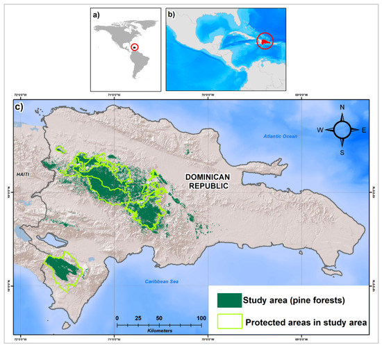
Figure 1.
Study area (a) general location of the Dominican Republic, (b) regional location, and (c) study area including the protected areas.
The study was carried out in the pine forests of the Dominican Republic, which cover 3287 km2. Most of this area lies in the Cordillera Central (the highest elevation mountain range on the island) and comprises four large protected areas that were declared national parks (NPs): (i) NP Armando Bermúdez, (ii) NP José del Carmen Ramírez, (iii) NP Valle Nuevo, and (iv) NP Sierra de Bahoruco.
The water service for human consumption and agricultural use in most of the country is one of the main environmental services offered by the Central Cordillera to the Dominican Republic. The vegetation patterns vary mainly due to large-scale climatic factors, such as the direction of the northeast or southeast winds. This mountain range features the principal pine forests of the country. The higher sites of the mountain range include moist broadleaf forests, while the windward side includes forests of West Indies pine (Pinus occidentalis Swartz) [29]. This pine is endemic to the island of Hispaniola (19°N, 71°W), although it has been known to scientists for more than 200 years and still covers extensive areas of the Dominican Republic and Haiti [30].
Recent studies conducted under the REDD+ program by the Ministry of the Environment and Natural Resources (MARN) have indicated that the illegal extraction of wood for firewood and charcoal to be used as fuel, timber, and weak management are the principal drivers of pine forest degradation in the Dominican Republic [31].
2.2. Forest, Deforestation, and Degradation Definitions
In recent times, the definition of ‘forest’ has taken on particular relevance due to the challenges of countries to monitor the CO2 emissions from the forest sector as part of the objectives to establish robust MRV systems for REDD+. In general, the definitions of ‘forest’ include references to threshold parameters that include the minimum area of land, minimum tree height, and minimum canopy cover. Many countries are aligned with the minimum thresholds described by the United Nations Food and Agriculture Organization’s (FAO) Global Forest Resource Assessment (FRA). Through the FRA, since 2000, all countries have aligned themselves to adopt a definition of ‘forest’ with common parameters, such as (i) a canopy coverage of more than 10%, (ii) trees of 5 m, and (iii) land of at least 0.5 ha [32]. The present study subscribes to the definition of ‘forest’ adopted by the Dominican Republic, with a focus on pine forests in accordance with the Reference Emission Levels/Forest Reference Levels (FREL/FRL): “land of at least 0.5 ha covered by pine trees higher than 5 m and with a canopy cover of more than 30%, or by trees able to reach these thresholds, and predominantly under forest land use, this excludes land that is mainly under agricultural or urban land uses” [33].
Based on the definition of forest described above, in the current study, forest degradation is defined as “the loss of carbon content in forest lands that remain as forest lands with a decrease in canopy cover that does not qualify as deforestation and that can be caused by anthropogenic activities”. Forest degradation has a human-induced negative impact on carbon stock changes; our operational definition for measuring forest degradation is based on indicators, such as forest structure (changes in canopy cover) [34] that affect the ability of the forest to store carbon under natural conditions [35]. These definitions demonstrate that deforestation and forest degradation involve different conditions, processes, and concepts. Deforestation suggests a change in land use from forest to non-forest land use, altering the original structure and environment of the forest, while degradation occurs in forest lands that are maintained as forest lands but suffer losses in their forest ecosystem functions (Figure 2).
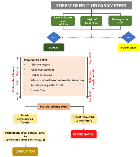
Figure 2.
Main parameters and elements that interact in forest degradation in the Dominican Republic.
2.3. Method
Once the baseline data were collected and the key concepts (forest, deforestation, and forest degradation) were defined, a method to quantify the degradation of pine forests in the Dominican Republic was developed. The overall structure of the method (Figure 3) consists of four stages: (i) the preprocessing and selection of Landsat images, (ii) the computation of the spectral indices to map land cover for the 1990–2018 period, (iii) changing the magnitude of mapping, and (iv) mapping the carbon stocks in pine forests. The entire process was accompanied by an accuracy analysis for each step in which a classification, probability, and regression model was applied using the Smile random forest (RF) algorithm. The GEE cloud-based platform was also used in our research.
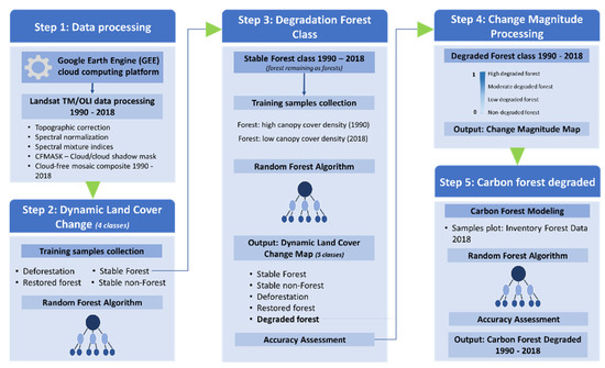
Figure 3.
Flowchart: representation of the methodology used in our research.
Our models were developed using the Landsat Thematic Mapper (TM) and an operational land imager (OLI) by applying the RF algorithm in GEE to generate a dynamic land cover change map, degraded forest map, and carbon forest map. The model was trained and validated using sample plots from the forest inventory and satellite images.
2.4. Reference Data
2.4.1. Landsat TM/OLI Data Processing
We used Landsat-5 TM and Landsat 8 OLI surface reflectance data with 16 day and 30 m resolutions (available in the GEE computing platform) [21]. All Landsat-5TM surface reflectance data from year 1990 ± 0.5 (a total of 22 images) and Landsat-8 OLI surface reflectance data from year 2018 ± 0.5 (a total of 322 images) available in GEE were used in this study.
The Landsat surface reflectance data in GEE were atmospherically corrected using the Landsat Ecosystem Disturbance Adaptive Processing System (LEDAPS) (TM) and Landsat Surface Reflectance Corrected (LaSRC) (OLI) algorithms [36,37]. The CFmask algorithm was used to mask the clouds and cloud shadows [38,39]. Landsat 5 TM Top of Atmosphere (TOA) and OLI TOA collections were also used [40].
Digital elevation data were obtained from the Shuttle Radar Topography Mission (SRTM) [41] in GEE. These data have a 30 m spatial resolution. SRTM data were used to calculate the topographic slope and elevation. In addition, the empirical Earth rotation model (ERM) was used as a basis to apply a terrain illumination correction algorithm [42], which allowed us to topographically correct each image. For reflectance images, we used the medoid method [43] (Figure 4).
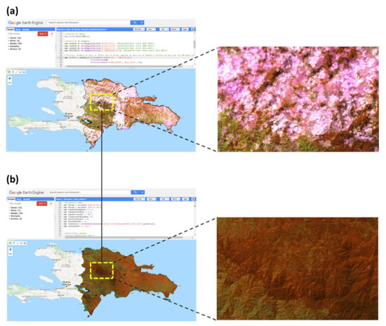
Figure 4.
Mosaic of seasonal images for the Dominican Republic in 2018. (a) Original composite mosaic, (b) medoid composite (shortwave infrared 1 (SWIR1), near-infrared (NIR) and red band).
Once the images were preprocessed, a composite mosaic was developed. This mosaic was formed by combining spatially overlapping images into a single image based on a function of multiple spectral and temporal aggregation ranges [44]. This mosaic (multiband and multidate) was built with the images of the years 1990 and 2018.
2.4.2. Field Inventory Data
The reference field data included in this study are based on the National Forest Inventory (NFI) collected by the Ministry of the Environment and Natural Resources (MARN) of the Dominican Republic with the support of the REDD/CCAD-GIZ program and the World Bank’s Forest Carbon Partnership Facility (FCPF) (https://www.forestcarbonpartnership.org/country/dominican-republic (ERPD document, September, 2019)) [45]. In 2012, the Dominican Republic designed its MRV strategy. This strategy proposed two major lines of monitoring forest resources: (i) satellite monitoring and (ii) terrestrial monitoring. For terrestrial monitoring, the country executed an NFI between 2017 and 2018 with a plan to develop permanent sampling plots to be measured every 5 years according to the action plan of the country’s MRV System. The NFI of the Dominican Republic contains 404 sampling units located in the different forest classes, such as moist broadleaf forests (204 plots), subdivided into semi-humid broadleaf forests (117 plots), humid broadleaf forests (76 plots), and broadleaf cloud forest (11 plots); pine forests (59 plots), subdivided into high canopy cover density (19 plots) and low canopy cover density (40 plots); dry forests (71 plots); and mangrove forests (70 plots).
The plot is rectangular with a size of 0.125 hectares (ha) (25 m × 50 m). Different forest characteristics and topographical factors were measured at all plots (tree species, height, diameter at breast height (DBH), soil organic matter, number of trees, geographical coordinates, elevation, and slope). To design the NFI, the methodology proposed by the REDD/CCAD-GIZ program was used [46,47]. For our study, we used the data from 51 plots located in the pine forest areas. More information about the methodology and the results of the NFI is available in the FREL/FRL submission of the Dominican Republic [33,48] to REDD+ UNFCCC (Figure 5) (Appendix D Table A2 and Appendix E Figure A1).
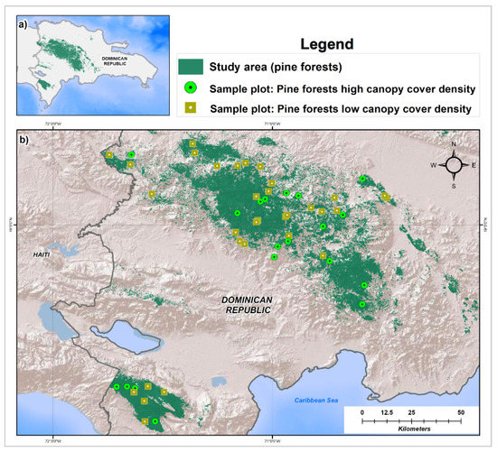
Figure 5.
(a) General location of the Dominican Republic; (b) location of permanent plots in pine forests with low and high canopy cover density.
2.5. Classification of Dynamic Land Cover Change
One of the most relevant tasks for RS is land cover mapping. Different spectral indices are used to improve such mapping techniques [49]. For land cover change mapping, we generated a composite mosaic for the 1990–2018 period, and spectral indices were selected based on the known characteristics of land cover classes. Landsat time series and spectral analyses were used to detect deforestation and degradation forests.
Classes that were determined in the dynamic land cover map correspond to a stable forest, stable non-forest, degradation, deforestation, and restored forest. Seven different vegetation indices were used to monitor the dynamics of forest change during the 1990–2018 period. Among the most relevant indices used are the enhanced vegetation index (EVI), which was designed to enhance the vegetation signal with improved sensitivity in high biomass areas [50]; the soil adjust vegetation index (SAVI) [51]; and the normalized difference fraction index (NDFI), which was constructed to highlight degraded or cleared forest areas. The NDFI values in intact forests are expected to be high (i.e., approximately 1) due to the combination of high “green vegetation” (GV) and low non-photosynthetic vegetation (NPV) and soil values [52]. The spectral indices used are closely related to the land cover defined in our research; Appendix C, Table A1 details each index used.
Land Cover Change Samples
Training samples for land cover change classification were derived from a visual analysis using Landsat from GEE and high spatial resolution images from Google Earth (GE) (Figure 6).
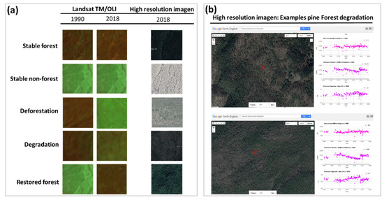
Figure 6.
Example of the image composites of different land cover dynamic change classes for pine forests of the Dominican Republic. (a) NIR-SWIR1-RED Landsat Thematic Mapper (TM) and Operational Land Imager (OLI) versus a high-resolution image; (b) example of degraded pine forests observed using Google Earth Engine (GEE).
First, we established four cover change classes: stable forest, stable non-forest, deforestation, and forest restoration. We allocated 97 samples to areas that appeared to be stable forest or stable non-forest, and the remaining 15 samples were allocated to land cover change. The second step was to detect forest degradation based on the stable forest class, commonly called the ‘forest mask’, following the criteria established in the definition of a forest in our study. We focused on two classes: non-degraded forest and degraded forest. A total of 90 samples were allocated to areas with disturbances observed in the 1990–2018 period. Reference samples were randomly distributed over each land cover class in the study area, while a single pixel was used as the sample unit (Figure 7).
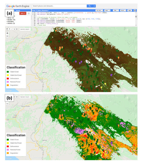
Figure 7.
Training samples of 5 land cover classes in GEE: (a) samples of land cover change class; (b) dynamics of land cover change classification.
The training dataset was used to improve the supervised classification, the per-band pixel values of the stacked composite images were extracted from the training samples, and the resulting data were used to train the RF classifiers [53]. We used the RF algorithm, because it is a built-in classifier in GEE and has been widely demonstrated to improve the accuracy of maps by combining random subsets of trees to classify the training samples. In GEE, the RF algorithm is applied through the following function: (ee.Classifier.smileRamdomForest). Moreover, the algorithm can be configured in three ways (ee.setOutputMode) based on the classification mode (class/type maps), regression mode (maps with continuous values predicted), and the probability mode (map with rescaled values between 0 and 1). In the current study, the RF algorithm was applied in the classification mode using GEE to obtain the land cover, in the regression mode to estimate the carbon maps, and in the probability mode to estimate the change magnitude maps.
2.6. Carbon Stock and Change Magnitude
Estimating the spatial–temporal distributions of forest carbon stocks subject to land cover changes is critical for estimating and reporting GHG emissions [54]. To spatially represent explicit forest degradation along with degraded carbon, we generated a carbon map of pine forests using 51 sampled plots from the NFI data and Landsat 2018.
The size of each parcel is 0.125 hectares (ha) (25 m × 50 m). As the size of each plot and the Landsat pixels do not match, we used the geographic coordinates of the centroid of the plot. Thus, we applied the carbon values in units per hectare (t ha−1) to each pixel.
For each plot, four of the five C pools were measured [55]: aboveground biomass (AGB), belowground biomass (BGB), deadwood (DW), and leaf litter (Table 1) [47,56,57] (See Section 2.4.2 Field Inventory Data for more details). To convert the biomass to carbon, the IPCC default carbon factor value (0.47) was used. Each pool was modeled independently using spectral responses (vegetation indices) from Landsat, applying a regression model with the RF algorithm in GEE (ee.Classifier.randomForest(30).setOutputMode(‘REGRESSION’). Through this process, each spatial pixel acquired an AGB (t C ha−1) value and its related standard deviation as a measure of uncertainty. The code generated to model the C stock using the GEE is available in Appendix B.

Table 1.
Definitions and variables used to estimate the carbon stored in the pine forest.
The change magnitude is assumed to be an approximate indicator of the amount of tree removal or canopy damage that occurred due to disturbances [58]. The change magnitude was estimated from the spectral indices for the stable forest class using the composite mosaic for the 1990–2018 period. We fitted an RF probability model in GEE to represent the structural forest changes in each of the spectral indices described previously (ee.Classifier.randomForest(50).setOutputMode(‘PROBABILITY’).
The disturbance monitoring algorithm used to identify the forest changes in each pixel location is closely related to the Continuous Change Detection and Classification algorithm (CCDC) [20,58,59] but was adapted using RF models to predict the change magnitude probabilities for bitemporal observations. Several studies have successfully applied this algorithm to different sensors and different spectral indices to detect changes [60,61]. This change detection algorithm operates on the time series of each pixel in the study area.
The decrease in a spectral index caused by a disturbance is recognized by a certain change magnitude. For example, values close to 1 in the NDFI spectral indices indicate high proportions of green vegetation (GV) or stable forests, while values close to 0 in the NDFI imply higher proportions of soil (So). The code generated to estimate the change magnitude using the GEE is available in Appendix B.
Pixel-based mapping facilitates comparisons and evaluations of changes with direct algebraic calculations [62]. Once the carbon stored in the four pools of the forest was estimated for the year 2018 along with the magnitude of change between 1990–2018, we used (Equation (1)) to determine the C stocks in each pixel for the year 1990. Finally, the degraded carbon was estimated as the difference of the C stored in the pine forests between 1990 and 2018 combined with the change magnitude observed in the same period (Equation (2)). To estimate forest degradation, only disturbances occurring in the stable forest class were considered for the period analyzed:
where is the C stock in 1990 (Mg ha−1), is the C stock in 2018, and is the change magnitude (value > 0 and < 1).
where is the carbon degraded for the 1990–2018 period (Mg ha−1), is the C stock in 1990, and is the C stock in 2018.
Finally, to calculate the annual rate of degraded carbon, the stock-difference method (SDM) was used, where changes in carbon stock (∆Carbon) represent the difference between carbon stocks for a given forest area estimated at two time points (Equation (3)):
where is the annual change in C stocks (Mg·C·ha−1·yr−1), is the C stock in 1990 (Mg·C·ha−1), and is the C stock in 2018 (Mg C·ha−1).
2.7. Model Evaluation: Carbon Stock
Cross-validation (CV) is one of the most commonly used techniques to evaluate the efficiency of a machine learning (ML) technique; this is due to its wide application in the scientific arena and its efficiency in detecting a model’s overfitting problems [63]. To evaluate the performance of the machine learning model applied to map the change magnitude and forest carbon, the following functions were used: coefficient of determination (R2), mean square error (MSE), root mean square error (RMSE), mean absolute deviation (MAD), cumulated forecast error (CFE), and mean absolute percentage error (MAPE):
where is the number of samples used for the machine learning model, is the value observed (C stock), is the corresponding mean value, is the predicted value (C stock), and is the mean value.
2.8. Accuracy Assessment and Analysis
We used the confusion matrix statistical accuracy assessment method to evaluate the dynamic land cover change classification. The overall accuracy (OA), user’s accuracy (UA), and producer’s accuracy (PA) were applied to each class, and the Kappa coefficient was used to assess the class map and determine the level of agreement between two raters. The standard deviations and the confidence intervals (at a 95% significance level) were also estimated.
Since land change classes (degradation, deforestation, and forest restoration) tend to cover only a small portion of the study objectives compared to stable areas (stable forest and stable non-forest), it is recommended to stratify the study based on a map that represents the classes of principal interest to ensure an effective statistical sample representation in land change classes, such as degradation, deforestation, and forest restoration [64].
An accuracy assessment of the dynamic land cover change map (for the 1990–2018 period), generated through a sampling-based approach to estimate the area of forest degradation in the Dominican Republic (Figure 6), was performed on the following land cover change classes:
Stable forest: pine forests that remain pine forests without disturbance; this forest contains over 30% canopy cover.
Stable non-forest: other non-forest lands, such as agriculture, wetlands, grasslands.
Deforestation: elimination of the forest canopy cover that exceeds 30%; results in a land-use change.
Degradation: this entails any disturbance that changes the canopy cover density between 100% and 30% and does not result in a land-use change.
Forest restoration: conversion of non-forested land to forest; this includes forest restoration with a canopy cover greater than 30% (through natural and artificial means) on deforested land.
For the accuracy assessment, a total of 1124 spatial sampling points (Table 2) were established for the study area using the stratified random sampling approach following best practices [64] (Equation (10)). It was necessary to modify the minimum sample size to determine the objective standard error of the degradation area, rather than the OA of the map, and thereby ensure that sample size would be large enough to produce sufficiently accurate estimates [65]. The stratified area estimator-design tools hosted in the System for Earth Observation Data Access, Processing and Analysis for Land (SEPAL) were used to generate random spatial points (Table 2). SEPAL is a cloud-based computing platform developed by FAO, which uses the GEE and OpenForis Geospatial Toolkits [66].
where number of points in the study area, is the standard error of the estimated OA, is the mapped proportion of the class area , and is the standard deviation of land cover classes .
Table 2.
Strata area, sample allocation for the stratified random sample, and weights for the study period (1990–2018).
We performed an analysis following best practices to assess the accuracy of the map classification, and the area of change was estimated using a classification error matrix. For details on the matrix nomenclature, refer to Olofsson et al. (2014) [64].
Collecting reference observations of forest degradation is a complex task, primarily because degradation is a continuous process that must be observed over a long period. In this sense, satellite images with high spectral resolutions have become a key tool, but they are not sufficient to reconstruct the landscape’s historical dynamics. Therefore, this study required the use of a Landsat observation time series supported by very high spatial resolution (VHRS) imagery. Independent stratified validation samples were visually interpreted from the VHRS time-series images of Collect Earth (CE). We built a survey in CE that helped us access multiple satellite images, including archives including VHSR imagery (Google Earth, Bing Maps) and a set of satellite images from the GEE catalog, along with their derived spectral indices [67] (Figure 8).
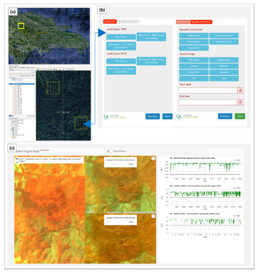
Figure 8.
Tools used to collect the reference observations of forest degradation. (a) Collect Earth interface in Google Earth Pro; (b) Collect Earth survey; (c) time series tools online viewer.
To facilitate the historical collection of reference data, other GEE assessment tools were adapted and used, such as the Accuracy and Area Estimation Toolbox (AREA2) developed by Bullock and Olofsson (2018) (see github.com/bullocke/AREA2). The sample interpretation tool allowed us to determine reference labels for the 1124 samples collected. This algorithm helped estimate the map accuracy and disturbance area and visualize the time series trends of each sample using a dataset created using the Continuous Degradation Detection (CODED) methodology in GEE [20] (see Appendix B for the code developed in this study using the GEE).
To review and assign reference labels to each of the 1124 selected special sample units, three trained interpreters were delegated. These interpreters did not know the classes of the assigned samples. An additional interpreter reviewed all samples with low or medium confidence. At least three interpreters reviewed all units labeled as degradation. The decision matrix and labels assigned to the samples evaluated in the time series are shown in Table 3.
Table 3.
The decision matrix for the validation samples interpreted from high-resolution images and a Landsat time series using Collect Earth (CE) and GEE, respectively.
3. Results
3.1. Dynamic Land Cover Changes from 1990 to 2018
The total study area corresponded to 328,777 ha of pine forests in the Dominican Republic. The results showed that degraded forests accounted for 11% ± 1.21% (95% confidence interval) of the total study area between 1990 and 2018, while 79% ± 1.28% remained stable and did not suffer any disturbances; further, 2% ± 0.61% were deforested. In total, we estimated that 36,808 ± 446 ha of pine forests was degraded.
The margin of error of the area estimate for forest degradation was 10.8% (95% CI). The user’s accuracy was 70.7%, and the producer’s accuracy for forest degradation was 91.3%. The overall accuracy of the dynamic land cover change map was 92.8%. The main results corresponding to the accuracy assessment are shown in Table 4.
Table 4.
Confusion matrix—sample counts, area proportions, area estimates, and accuracy measures for stable forest, stable non-forest, deforestation, restored forest, and forest degradation.
We analyzed the dynamics of land cover change, as they relate to the country’s protected areas, and identified that 71% of the degraded pine forests exist within the protected area. Among these, the main forest belongs to Sierra de Bahoruco National Park (NP), with 14,166 ha (30% of the total degraded area), followed by Valle Nuevo NP and José del Carmen Ramírez NP, with 8,736 ha (18% of the total degraded area) and 6,462 ha (16% of the total degraded area), respectively. Table 5 shows the locations of the protected areas with the degraded pine forests from 1990 to 2018. A geographic representation of the dynamic land cover change map obtained in our study is also provided (Figure 9). Detailed results on land cover change are available via a dashboard called “Accuracy assessment and analysis tools” available in Appendix A.
Table 5.
Dynamics of land cover change associated with the different classes of protected areas in the Dominican Republic.
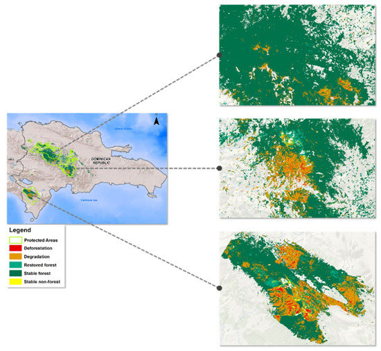
Figure 9.
Dynamic land cover change map for the 1990–2018 period.
3.2. Carbon Stock
The total carbon stock in the pine forest area analyzed was composed of AGB C, BGB C, DW C, and litter C pools. The results for the total carbon analysis are presented in Table 6, Figure 10, Figure 11 and Figure 12. The analysis shows that the total carbon stock in 2018 was approximately 19,002,000 Mg C, with an average of 64.4 Mg C ha−1. The RMSE of the model was 13.4 Mg C ha−1, the R2 was 0.78, the CFE was 0.35, and the MAPE reached 21%. Of the total carbon stock stored, 75.8% (14,410,609 Mg C) was in the National Park, while 18.4% (3,498,042 Mg C) was outside protected areas, and 4.3% (824,182 Mg C) was stored in natural reserves (Table 7). Detailed results on the carbon stored from the different pools and protected area categories are available via a dashboard provided in Appendix A.
Table 6.
Results of the accumulated carbon stock model, carbon stock for the different pools estimated, and their error measures based on random forest modeling.
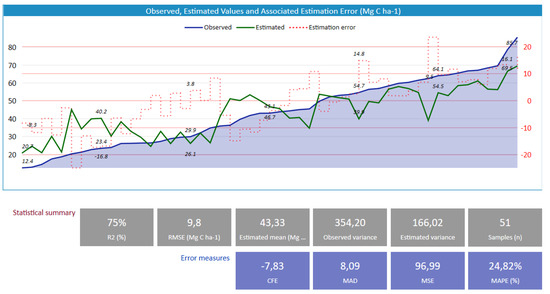
Figure 10.
Carbon stored in the pine forests in 2018—a statistical summary and the error measures used to evaluate the performance of the model via random forest modeling.
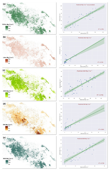
Figure 11.
Spatial distribution of the average predicted carbon stocks in pine forests (zoomed in image of the national parks with the highest density of pine forests) and the carbon prediction graph with a 95% confidence interval: (a) total carbon; (b) litter C; (c) AGB C; (d) downed dead C; (e) BGB C (Note: 1 Mg ha−1 = 1 ton ha−1).
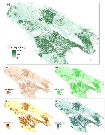
Figure 12.
Spatial distribution of degraded carbon (zoomed-in image of the Sierra de Bahoruco National Park protected area with the highest degradation): (a) total carbon; (b) AGB C; (c) BGB C; (d) DW C; (e) litter C in the pine forests of the Dominican Republic.
Table 7.
Results of the accumulated carbon stocks and carbon stock models for the different pools in each protected area category.
3.3. Carbon Degraded in the 1990–2018 Period
The total carbon degraded in the pine forest area analyzed was 3,479,159 Mg C. Converting this degraded carbon into emission- and climate-related units of CO2-equivalent emissions (metric tons CO2-equivalent units), the emissions caused by the degradation of the pine forests in the period 1990–2018 were 12,756,916 tCO2eq, with an annual average of 2.6 Mg C ha−1 yr−1 (9.5 tCO2eq ha−1 yr−1). Of the total degraded C stock, 73.9% (2,570,081 Mg C) was found in national parks, while 2.9% (102,401 Mg C) and 22.8% (792,048 Mg C) of C were degraded in natural reserves and non-protected areas, respectively (Table 8). Detailed results on the degraded carbon in pine forests in the 1990–2018 period for the different pools and protected area categories are provided in Appendix A.
Table 8.
Results of degraded carbon for different pools per protected area category.
4. Discussion
4.1. Validation of Dynamic Land Cover Change Map from the 1990–2018 Period
Most of the countries that are part of the REDD+ mechanism do not quantify or report their emissions caused by forest degradation [16]. Efforts to find such a method have been great, and the challenge of obtaining accurate estimates remains under investigation and debate in the scientific arena. One of the main agreements in the measurement and monitoring of forest degradation is that a long series of temporal and spatiotemporal observations are required to detect disturbances in forest cover, which is why satellite images, such as those from Landsat, are key inputs to establishing more robust MRV systems for REDD+.
Using Landsat data in GEE, we developed a methodology to monitor pine forest degradation in the tropics. This approach was determined to be precise, with an overall 92.9% and 91% producer’s accuracy in the degraded forest class of the dynamic land use change map of pine forests in the Dominican Republic. Our estimates of forest degradation are compatible with those of other studies on a sub-national scale. For example, the OA obtained in degradation and deforestation mapping in Rondônia, Brazil, was 91%, while the producer’s accuracy reached 68% in the forest degradation class [58]. In the forests of the Brazilian Amazon, the OA in degradation and deforestation mapping was 92%, while the producer’s accuracy was 80% in the forest degradation class [68]. Another study using SPOT images with spectral mixing models in the eastern Amazon showed results that also indicated good agreement (86% OA) [69].
The dynamic mapping analysis determined an efficient stratification in the study area and allowed for an impartial estimation. Margins of error of 10.8% were obtained when mapping forest degradation at a 95% confidence level. Although the mapping of forest degradation in tropical forests is scarce in the literature, we observed some consistency between our results and those of other studies in the temporal scale, spatial and spectral resolution of the images used, accuracy, and the use of vegetation index analysis as a method to evaluate and map tropical forest disturbances.
Historical data collection on forest changes is a challenging task because such data are not readily available everywhere, and temporal change data are not detailed enough for the validation of time series maps. The current study used the AREA2 algorithm developed by Bullock and Olofsson (2018) by applying the Time Series Viewer. This is a sample interpretation tool used to determine the reference labels derived from a mapped dataset. However, a new challenge involved assessing the changes detected by the model. For this process, independent datasets were selected and assessed using CE [70]. The combination of these tools proved to be efficient in our study.
Using spectral index measures to validate the dynamic land cover change map in our study allowed us to extend tele-interpretation techniques and facilitated the visual detection of historical change processes, especially for degraded forest detection. In other research, the NDFI was used to map degradation; ultimately, the NDFI was found to be more sensitive to disturbances from tropical forests than other spectral indices [71]. We use different spectral indices to improve our estimates of forest degradation and performed a regression analysis with random forest to determine the importance of the indices in the constructed model. We found that the NDFI and EVI were the main variables able to explain the model and thereby classify areas with forest degradation for the 1990–2018 period (Figure 13a,b).
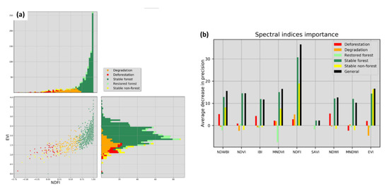
Figure 13.
(a) Scatterplot of two spectral indices (EVI and NDFI); the points represent the values of the most important variables used for land cover change classification; (b) spectral index importance analysis used for dynamic land cover change classification.
While the Dominican Republic has experienced a decrease in deforestation in recent times, forest degradation has been on the rise. In our study, we found that an area equivalent to 14% of pine forests of the Dominican Republic was degraded between 1990 and 2018. This is a critical element that must be considered for the development of a REDD+ program in the country. The Dominican Republic established a FREL/FRL to obtain results-based payments under the REDD+ mechanism supported by the FCPF. This includes emissions and removal in the remaining forest land (emissions from forest degradation) for the 2006–2015 period [45]. In this sense, the methodology proposed and the results obtained in the current study contribute directly to monitoring and quantifying CO2, emissions and removal. Furthermore, this methodology is a valuable tool that can be used in other tropical countries to monitor forest degradation.
4.2. Carbon Model Assessment
Forest inventory is an important source of information for a variety of strategic purposes in forest management. Based on 51 carbon samples obtained in pine forests, we generated a predictive regression model of the carbon stored in AGB, BGB, DW, and litter. Satisfactory results were obtained when applying the RF algorithm to estimate the total carbon stock in the study area, obtaining an R2 of 78.1% and an RMSE of 13.38 Mg C ha−1. It was determined that 19,002,000 Mg C is stored in the pine forests of which 3,479,159 Mg C was degraded (18% of C stock), which is equivalent to 124,255 Mg C yr−1 for the 1990–2018 study period.
We found some differences between our results and previous estimates; for example, the MARN of the Dominican Republic estimated the local emissions from forest degradation at a level of 182,937 Mg C yr−1, including all forest classes, and at a level of 46,591 Mg C yr−1 specifically for pine forests for the 2006–2015 reference period [33]. The differences between both estimates are mainly due to the scale of monitoring (sub-national vs. national), the methodology, the reference period, the algorithms used for image processing and classification, and especially the differences in the accuracy obtained between both estimates.
These differences also suggest that between 1990 and 2006, the degradation rate in the pine forest was much higher compared to that during the period 2006–2015. This provides a new research opportunity to understand the drivers of degradation that have decreased in the country. However, we believe that the degradation estimates found in both studies differ from each other due to the previously mentioned technical and methodological factors.
A robust and transparent national forest monitoring system to monitor and reporting five REDD+ activities is required [9]. Often, capabilities and national circumstances prevent the monitoring and reporting of CO2e emissions and their removal under the five REDD+ activities. In our study, the forest carbon stock increases in forest lands that remain forest lands were not estimated for the reference period due to the absence of information on the average annual increase in biomass in the studied forest. This offers a new research opportunity for a “step-wise” approach that will allow estimate net CO2e emissions as part of one of the five REDD+ activities called “enhancement of forest carbon stocks”.
4.3. Google Earth Engine Platform
The processing and analysis of the data from our study were accomplished using the JavaScript API via the code editor of the GEE platform. Using GEE, the processing time efficiency increased, and satisfactory results were obtained (see the GEE code developed for this study in Appendix B). GEE is considered a multidisciplinary tool; since 2017, its application has increased notably, especially in land-use mapping and water resources. Landsat images (82%), the RF algorithm (52%), and the NDVI spectral indices are the most frequently used methods in recent studies related to vegetation [72].
In our study, we faced a series of complexities in the detection of forest degradation, especially since a very detailed approach is required. This approach involves detecting the reduction or modifications in the forest structure that are not considered a total loss over an extended period of time and at a large scale. Using the characteristics of the GEE platform by extracting spectral characteristics from satellite images, it was possible to satisfactorily solve the main challenges we encountered.
The methodology proposed here was able to detect the dynamics of change in land use and forest degradation. While there is room to improve the methodology, the use of GEE with its computing capacity and the availability of free satellite images provide powerful support for mapping forest degradation. Additionally, GEE allowed us to quantify the carbon stored until 2018 and the degraded carbon in four pine forest pools. Thus, this method could become a key monitoring tool (at the sub-national and national levels). Moreover, this tool will allow authorities to monitor forest degradation according to indicator 15.3.1 of the Sustainable Development Goals (SDGs), which defines the area of degraded land and will serve as an essential element for developing national MRV systems for REDD+ strategy implementation and supporting the report on GHG emissions of the United Nations Framework Convention on Climate Change (UNFCCC) in an efficient, robust, and transparent manner.
5. Conclusions
The current study developed and applied a methodology for forest degradation mapping based on available data from the Open Access Landsat and the GEE platforms. Additionally, GEE was used in combination with tools, such as SEPAL and CE by the FAO. The main objective was to estimate the degraded pine forest area and quantify the degraded carbon for a period of 28 years (1990–2018) by applying machine learning models, such as random forest.
The methodology applied in this study shows new possibilities for forest degradation monitoring and estimating CO2 emissions from forest degradation using spectral information derived from Landsat archives and data from the forest inventory; combining both sources of information can also help improve the MRV systems for the REDD+ mechanism.
The model assessment revealed a dynamic land change map with a cumulative overall accuracy of 92%, in relevant classes (such as forest degradation) with a UA of 70.7%, and a PA of 91.2%. A carbon stock model was also developed with an R2 of 79% to estimate degradation in terms of the Mg C ha−1. The applied models were built, trained, and validated to demonstrate the efficiency of the methodology. The results obtained indicate that this methodology can be an especially useful tool for time series processing to map forest degradation by applying technologies, such as GEE.
GEE has excellent potential for the “wall to wall” forest degradation mapping of tropical pine forest ecosystems. More research is still required to assess the ability of GEE to map degradation in broadleaf forests and dry forest ecosystems by applying machine learning techniques combined with spatial data and field measurements. The approaches presented herein could become a key tool for measuring and monitoring emissions from forest degradation in the tropics.
Author Contributions
Conceptualization, E.D., F.D., F.C., and E.Z.; methodology, E.D., J.A.B., F.C., and A.J.H.; software, E.D. and F.C.; validation, E.D. and F.C.; analysis, E.D., F.C., J.A.B., F.D., A.J.H., and E.Z.; investigation, E.D., F.C., J.A.B., F.D., A.J.H., and E.Z.; writing—original draft, E.D., F.C., J.A.B., F.D., A.J.H., and E.Z.; supervision, E.D., F.C., J.A.B., F.D., A.J.H., and E.Z. All authors have read and agree to the published version of the manuscript.
Funding
This research was funded by the National Agency for Research and Development of Chile (ANID) www.anid.cl.
Acknowledgments
We are sincerely grateful to the National Forest Monitoring Unit of the Ministry of Environment and Natural Resources (MARN) of the Dominican Republic, Sud Austral Consulting, and the REDD/CCAD-GIZ program for the information and technical support they provided. Special thanks to the Faculty of Agronomy, University of Concepción, for funding a training internship at Utah State University. We also thank the editor and reviewers for their comments on this paper.
Conflicts of Interest
The authors declare no conflict of interest.
Appendix A
A consolidation of the results obtained is available on a dashboard with free online access called “Accuracy assessment and analysis tools”. This dashboard presents assessments of the dynamic land cover change, the spectral mixture analyses from Landsat, the error matrix, the carbon model, and all the results obtained. The dashboard allows users to pose questions and filter graphic and alphanumeric data with a geographic viewer. The dashboard is available at the following link: Accuracy assessment and analysis tools.
Appendix B
The codes developed in this study using the GEE cloud-based computing platform are available at the following link: Degradation code.
Appendix C
Table A1.
Spectral indices used for forest degradation mapping.
Table A1.
Spectral indices used for forest degradation mapping.
| Spectral Indices | Equation |
|---|---|
| Normalized Difference Vegetation Index (NDVI) [73] | |
| Normalized Difference Spectral Vector (NDSV) [74] | where and are two generic bands. |
| Enhanced Vegetation Index (EVI) [50] | |
| Soil Adjust Vegetation Index (SAVI) [51] | |
| Index-Based Built-Up Index (IBI) [52] | |
| Near-Infrared Reflectance of Vegetation (NIRv) [75] | |
| Normalized Difference Fraction Index (NDFI) [52] | where: |
Appendix D
Table A2.
Reference field: National Forest Inventory (NFI) collected by the Ministry of the Environment and Natural Resources (MARN) of the Dominican Republic.
Table A2.
Reference field: National Forest Inventory (NFI) collected by the Ministry of the Environment and Natural Resources (MARN) of the Dominican Republic.
| ID | Class | AGB (Mg C ha−1) | BGB (Mg C ha−1) | Litter (Mg C ha−1) | DW (Mg C ha−1) | Total Accumulated (Mg C ha−1) | Long | Lat |
|---|---|---|---|---|---|---|---|---|
| 1 | Pine forest: low canopy cover density | 18.6 | 7.9 | 0.4 | 0.0 | 37.5 | −71.363 | 19.371 |
| 2 | Pine forest: high canopy cover density | 26.2 | 7.2 | 1.3 | 0.0 | 35.2 | −71.642 | 19.321 |
| 3 | Pine forest: low canopy cover density | 12.4 | 4.6 | 0.5 | 0.3 | 22.2 | −71.743 | 19.321 |
| 4 | Pine forest: low canopy cover density | 17.4 | 5.3 | 0.6 | 1.2 | 26.8 | −71.354 | 19.330 |
| 5 | Pine forest: low canopy cover density | 34.8 | 11.3 | 0.6 | 2.2 | 56.1 | −71.647 | 19.277 |
| 6 | Pine forest: low canopy cover density | 85.7 | 25.0 | 3.3 | 2.9 | 123.6 | −71.158 | 19.272 |
| 7 | Pine forest: low canopy cover density | 56.4 | 15.3 | 2.6 | 2.7 | 77.4 | −71.055 | 19.268 |
| 8 | Pine forest: low canopy cover density | 49.8 | 15.6 | 1.8 | 2.2 | 77.5 | −71.122 | 19.284 |
| 9 | Pine forest: low canopy cover density | 41.8 | 12.0 | 0.9 | 7.7 | 65.2 | −71.252 | 19.270 |
| 10 | Pine forest: high canopy cover density | 43.0 | 13.2 | 4.6 | 2.5 | 69.3 | −70.589 | 19.212 |
| 11 | Pine forest: low canopy cover density | 29.6 | 10.3 | 0.4 | 0.1 | 49.1 | −71.001 | 19.191 |
| 12 | Pine forest: high canopy cover density | 58.4 | 17.5 | 4.1 | 0.5 | 86.8 | −71.054 | 19.107 |
| 13 | Pine forest: high canopy cover density | 27.3 | 8.5 | 3.1 | 0.8 | 43.7 | −70.936 | 19.146 |
| 14 | Pine forest: high canopy cover density | 64.1 | 20.2 | 3.8 | 0.8 | 99.8 | −70.881 | 19.134 |
| 15 | Pine forest: high canopy cover density | 68.4 | 20.6 | 1.4 | 4.4 | 102.8 | −71.033 | 19.119 |
| 16 | Pine forest: low canopy cover density | 60.3 | 17.9 | 5.0 | 3.7 | 92.7 | −70.478 | 19.124 |
| 17 | Pine forest: low canopy cover density | 59.8 | 17.3 | 1.2 | 2.4 | 84.8 | −70.488 | 19.134 |
| 18 | Pine forest: low canopy cover density | 23.4 | 9.2 | 0.9 | 4.0 | 48.3 | −71.073 | 19.131 |
| 19 | Pine forest: low canopy cover density | 45.4 | 12.3 | 1.3 | 27.4 | 86.4 | −70.717 | 19.125 |
| 20 | Pine forest: low canopy cover density | 29.9 | 8.1 | 0.3 | 0.0 | 38.2 | −71.550 | 19.143 |
| 21 | Pine forest: low canopy cover density | 52.1 | 15.9 | 1.1 | 4.4 | 80.2 | −71.017 | 19.154 |
| 22 | Pine forest: high canopy cover density | 53.5 | 15.2 | 1.3 | 4.9 | 77.9 | −71.159 | 19.055 |
| 23 | Pine forest: high canopy cover density | 45.1 | 14.9 | 1.6 | 2.8 | 74.5 | −70.679 | 19.046 |
| 24 | Pine forest: low canopy cover density | 39.6 | 12.6 | 0.8 | 0.0 | 60.1 | −71.067 | 19.022 |
| 25 | Pine forest: low canopy cover density | 32.0 | 9.2 | 5.6 | 0.7 | 49.5 | −70.706 | 19.066 |
| 26 | Pine forest: low canopy cover density | 78.7 | 22.2 | 3.0 | 2.9 | 110.2 | −70.824 | 19.079 |
| 27 | Pine forest: low canopy cover density | 26.3 | 7.3 | 3.2 | 5.8 | 43.4 | −70.941 | 19.039 |
| 28 | Pine forest: low canopy cover density | 35.9 | 11.0 | 2.6 | 29.3 | 83.4 | −70.933 | 19.046 |
| 29 | Pine forest: low canopy cover density | 20.3 | 5.9 | 5.4 | 0.8 | 33.7 | −70.775 | 19.061 |
| 30 | Pine forest: high canopy cover density | 43.8 | 13.7 | 17.9 | 0.1 | 82.3 | −70.769 | 18.994 |
| 31 | Pine forest: low canopy cover density | 43.1 | 11.9 | 0.9 | 0.3 | 57.3 | −71.073 | 19.013 |
| 32 | Pine forest: low canopy cover density | 61.5 | 17.1 | 0.6 | 8.2 | 89.1 | −71.167 | 18.967 |
| 33 | Pine forest: low canopy cover density | 21.2 | 6.1 | 0.6 | 1.6 | 30.8 | −70.925 | 18.952 |
| 34 | Pine forest: high canopy cover density | 69.6 | 18.8 | 0.7 | 4.4 | 93.6 | −70.975 | 18.902 |
| 35 | Pine forest: high canopy cover density | 56.9 | 15.8 | 0.7 | 11.3 | 86.5 | −70.929 | 18.926 |
| 36 | Pine forest: low canopy cover density | 28.8 | 9.9 | 0.4 | 0.1 | 47.2 | −71.148 | 18.927 |
| 37 | Pine forest: low canopy cover density | 64.5 | 17.4 | 0.2 | 0.0 | 82.1 | −71.126 | 18.913 |
| 38 | Pine forest: high canopy cover density | 62.5 | 18.6 | 0.7 | 0.9 | 89.3 | −70.738 | 18.836 |
| 39 | Pine forest: high canopy cover density | 66.8 | 18.8 | 0.0 | 0.2 | 88.5 | −70.992 | 18.855 |
| 40 | Pine forest: low canopy cover density | 23.8 | 7.9 | 0.3 | 0.0 | 37.3 | −70.770 | 18.861 |
| 41 | Pine forest: high canopy cover density | 22.7 | 6.5 | 1.0 | 0.0 | 31.8 | −70.581 | 18.726 |
| 42 | Pine forest: high canopy cover density | 36.3 | 12.5 | 1.0 | 1.3 | 60.9 | −70.590 | 18.639 |
| 43 | Pine forest: high canopy cover density | 67.1 | 19.0 | 1.2 | 11.0 | 101.6 | −71.709 | 18.263 |
| 44 | Pine forest: high canopy cover density | 53.1 | 17.6 | 3.0 | 1.1 | 86.7 | −71.662 | 18.263 |
| 45 | Pine forest: low canopy cover density | 26.4 | 8.6 | 1.0 | 1.0 | 42.4 | −71.568 | 18.265 |
| 46 | Pine forest: high canopy cover density | 65.5 | 19.6 | 0.8 | 1.0 | 94.1 | −71.625 | 18.256 |
| 47 | Pine forest: low canopy cover density | 14.4 | 6.0 | 0.6 | 0.0 | 29.1 | −71.493 | 18.238 |
| 48 | Pine forest: low canopy cover density | 12.8 | 4.2 | 0.3 | 2.0 | 22.1 | −71.584 | 18.197 |
| 49 | Pine forest: low canopy cover density | 26.1 | 13.5 | 1.1 | 0.9 | 65.7 | −71.631 | 18.239 |
| 50 | Pine forest: high canopy cover density | 54.7 | 19.4 | 1.3 | 1.7 | 94.5 | −71.534 | 18.105 |
| 51 | Pine forest: low canopy cover density | 44.4 | 13.9 | 0.8 | 0.0 | 66.1 | −71.581 | 18.104 |
Appendix E

Figure A1.
Reference map of the National Forest Inventory (NFI) collected by the Ministry of the Environment and Natural Resources (MARN) of the Dominican Republic.
Figure A1.
Reference map of the National Forest Inventory (NFI) collected by the Ministry of the Environment and Natural Resources (MARN) of the Dominican Republic.

References
- Friedl, M.A.; McIver, D.K.; Hodges, J.C.F.; Zhang, X.Y.; Muchoney, D.; Strahler, A.H.; Woodcock, C.E.; Gopal, S.; Schneider, A.; Cooper, A.; et al. Global land cover mapping from MODIS: Algorithms and early results. Remote Sens. Environ. 2002, 83, 287–302. [Google Scholar] [CrossRef]
- Wulder, M.A.; White, J.C.; Goward, S.N.; Masek, J.G.; Irons, J.R.; Herold, M.; Cohen, W.B.; Loveland, T.R.; Woodcock, C.E. Landsat continuity: Issues and opportunities for land cover monitoring. Remote Sens. Environ. 2008, 112, 955–969. [Google Scholar] [CrossRef]
- Pearson, T.R.H.; Brown, S.; Murray, L.; Sidman, G. Greenhouse gas emissions from tropical forest degradation: An underestimated source. Carbon Balance Manag. 2017, 12, 3. [Google Scholar] [CrossRef] [PubMed]
- Harris, N.L.; Brown, S.; Hagen, S.C.; Saatchi, S.S.; Petrova, S.; Salas, W.; Hansen, M.C.; Potapov, P.V.; Lotsch, A. Baseline Map of Carbon Emissions from Deforestation in Tropical Regions. Science 2012, 336, 1573. [Google Scholar] [CrossRef]
- Chazdon, R.L.; Brancalion, P.H.S.; Laestadius, L.; Bennett-Curry, A.; Buckingham, K.; Kumar, C.; Moll-Rocek, J.; Vieira, I.C.G.; Wilson, S.J. When is a forest a forest? Forest concepts and definitions in the era of forest and landscape restoration. Ambio 2016, 45, 538–550. [Google Scholar] [CrossRef]
- Arana Pardo, J.I.; Birdsey, R.; Boehm, M.; Daka, J.; Kobayashi, S.; Lund, H.G.; Michalak, R.; Takahashi, M. IPCC Report on Definitions and Methodological Options to Inventory Emissions from Direct Human-induced Degradation of Forests and Devegetation of Other Vegetation Types; Eggleston, H.S., Buendia, L., Miwa, K., Ngara, T., Tanabe, K., Eds.; Institute for Global Environmental Strategies (IGES): Kanagawa, Japan, 2003. [Google Scholar]
- van der Werf, G.R.; Morton, D.C.; DeFries, R.S.; Olivier, J.G.J.; Kasibhatla, P.S.; Jackson, R.B.; Collatz, G.J.; Randerson, J.T. CO2 emissions from forest loss. Nat. Geosci. 2009, 2, 737. [Google Scholar] [CrossRef]
- Metz, B.; Davidson, R.; Bosch, R.; Dave, R.; Meyer, L. Climate Change 2007: Mitigation of Climate Change; Cambridge University Press: Cambridge, UK, 2007. [Google Scholar]
- UNFCCC. Addendum Part Two: Action Taken by the Conference of the Parties at Its Sixteenth Session. In Proceedings of the Report of the Conference of the Parties on Its Sixteenth Session, Cancún, Mexico, 29 November–10 December 2011. [Google Scholar]
- Ochieng, R.M.; Visseren-Hamakers, I.J.; Arts, B.; Brockhaus, M.; Herold, M. Institutional effectiveness of REDD+ MRV: Countries progress in implementing technical guidelines and good governance requirements. Environ. Sci. Policy 2016, 61, 42–52. [Google Scholar] [CrossRef]
- Goetz, S.J.; Hansen, M.; Houghton, R.A.; Walker, W.; Laporte, N.; Busch, J. Measurement and monitoring needs, capabilities and potential for addressing reduced emissions from deforestation and forest degradation under REDD+. Environ. Res. Lett. 2015, 10, 123001. [Google Scholar] [CrossRef]
- Milne, R.; Jallow, P. Basis for Consistent Representation of Land Areas. In IPCC Good Practice Guidance for LULUCF; Institute for Global Environmental Strategies (IGES): Kanagawa, Japan, 2003. [Google Scholar]
- Woodcock, C. Free Access to Landsat Imagery Teach by the Book Science Education. Science 2008, 80, 1011–1012. [Google Scholar] [CrossRef]
- Hansen, M.C.; Potapov, P.V.; Moore, R.; Hancher, M.; Turubanova, S.A.; Tyukavina, A.; Thau, D.; Stehman, S.V.; Goetz, S.J.; Loveland, T.R.; et al. High-Resolution Global Maps of 21st-Century Forest Cover Change. Science 2013, 342, 850. [Google Scholar] [CrossRef]
- Herold, M.; Hirata, Y.; Laake, P.V.; Asner, G.; Heymell, V.; Román-cuesta, R.M. A review of methods to measure and monitor historical forest degradation. Unasylva 2011, 62, 16–24. [Google Scholar]
- Hosonuma, N.; Herold, M.; De Sy, V.; De Fries, R.S.; Brockhaus, M.; Verchot, L.; Angelsen, A.; Romijn, E. An assessment of deforestation and forest degradation drivers in developing countries. Environ. Res. Lett. 2012, 7, 044009. [Google Scholar] [CrossRef]
- Chambers, J.Q.; Asner, G.P.; Morton, D.C.; Anderson, L.O.; Saatchi, S.S.; Espírito-Santo, F.D.B.; Palace, M.; Souza, C., Jr. Regional ecosystem structure and function: Ecological insights from remote sensing of tropical forests. Trends Ecol. Evol. 2007, 22, 414–423. [Google Scholar] [CrossRef]
- De Sy, V.; Herold, M.; Achard, F.; Asner, G.P.; Held, A.; Kellndorfer, J.; Verbesselt, J. Synergies of multiple remote sensing data sources for REDD+ monitoring. Curr. Opin. Environ. Sustain. 2012, 4, 696–706. [Google Scholar] [CrossRef]
- Woodcock, C.E.; Macomber, S.A.; Pax-Lenney, M.; Cohen, W.B. Monitoring large areas for forest change using Landsat: Generalization across space, time and Landsat sensors. Remote Sens. Environ. 2001, 78, 194–203. [Google Scholar] [CrossRef]
- Zhu, Z.; Woodcock, C.E. Continuous change detection and classification of land cover using all available Landsat data. Remote Sens. Environ. 2014, 144, 152–171. [Google Scholar] [CrossRef]
- Gorelick, N.; Hancher, M.; Dixon, M.; Ilyushchenko, S.; Thau, D.; Moore, R. Google Earth Engine: Planetary-scale geospatial analysis for everyone. Remote Sens. Environ. 2017, 202, 18–27. [Google Scholar] [CrossRef]
- Azzari, G.; Lobell, D.B. Landsat-based classification in the cloud: An opportunity for a paradigm shift in land cover monitoring. Remote Sens. Environ. 2017, 202, 64–74. [Google Scholar] [CrossRef]
- Chen, B.; Xiao, X.; Li, X.; Pan, L.; Doughty, R.; Ma, J.; Dong, J.; Qin, Y.; Zhao, B.; Wu, Z.; et al. A mangrove forest map of China in 2015: Analysis of time series Landsat 7/8 and Sentinel-1A imagery in Google Earth Engine cloud computing platform. Isprs, J. Photogramm. Remote Sens. 2017, 131, 104–120. [Google Scholar] [CrossRef]
- Dong, J.; Xiao, X.; Menarguez, M.A.; Zhang, G.; Qin, Y.; Thau, D.; Biradar, C.; Moore, B. Mapping paddy rice planting area in northeastern Asia with Landsat 8 images, phenology-based algorithm and Google Earth Engine. Remote Sens. Environ. 2016, 185, 142–154. [Google Scholar] [CrossRef]
- Goldblatt, R.; Stuhlmacher, M.F.; Tellman, B.; Clinton, N.; Hanson, G.; Georgescu, M.; Wang, C.; Serrano-Candela, F.; Khandelwal, A.K.; Cheng, W.-H.; et al. Using Landsat and nighttime lights for supervised pixel-based image classification of urban land cover. Remote Sens. Environ. 2018, 205, 253–275. [Google Scholar] [CrossRef]
- Huang, H.; Chen, Y.; Clinton, N.; Wang, J.; Wang, X.; Liu, C.; Gong, P.; Yang, J.; Bai, Y.; Zheng, Y.; et al. Mapping major land cover dynamics in Beijing using all Landsat images in Google Earth Engine. Remote Sens. Environ. 2017, 202, 166–176. [Google Scholar] [CrossRef]
- Orvis, K.H. The highest mountain in the Caribbean: Controversy and resolution via GPS. Caribb. J. Sci. 2003, 39, 378–380. [Google Scholar]
- SEMARENA. Perfil Nacional Para Evaluar Las Capacidades Nacionales de Implementación del Principio 10 de la Declaración de Rio; Secretary of State for the Environment and Natural Resources: Santo Domingo, Dominican Republic, 2008; p. 119. [Google Scholar]
- Kennedy, L.M.; Horn, S.P.; Orvis, K.H. Modern pollen spectra from the highlands of the Cordillera Central, Dominican Republic. Rev. Palaeobot. Palynol. 2005, 137, 51–68. [Google Scholar] [CrossRef]
- Darrow, W.K.; Zanoni, T. Hispaniolan pine (Pinus occidentalis Swartz) a little known sub-tropical pine of economic potential. Commonw. For. Rev. 1990, 69, 133–146. [Google Scholar]
- MARN. Analysis of the Direct and Indirect Drivers of Deforestation and Forest Degradation (DD) in the Dominican Republic; Ministry of Environment and Natural Resources: Santo Domingo, Dominican Republic, 2018; p. 161. [Google Scholar]
- FAO. Global Forest Resources Assessment 2015; UN Food and Agriculture Organization: Rome, Italy, 2015. [Google Scholar]
- Feliz, K.; Rodríguez, L.; Galán, M.; Ovidio, R.; Vargas, O.; de Jong, B. Dominican Republic Reference Emissions Levels/Forest Reference Levels; Ministry of Environment and Natural Resources: Santo Domingo, Dominican Republic, 2019; p. 78. Available online: https://redd.unfccc.int/files/nrfe_-_nrf_rep._dom_revgov2.pdf (accessed on 18 March 2020).
- Romero-Sanchez, M.E.; Ponce-Hernandez, R. Assessing and Monitoring Forest Degradation in a Deciduous Tropical Forest in Mexico via Remote Sensing Indicators. Forests 2017, 8, 302. [Google Scholar] [CrossRef]
- Thompson, I.D.; Guariguata, M.R.; Okabe, K.; Bahamondez, C.; Nasi, R.; Heymell, V.; Sabogal, C. An Operational Framework for Defining and Monitoring Forest Degradation. Ecol. Soc. 2013, 18, 20. [Google Scholar] [CrossRef]
- Masek, J.G.; Vermote, E.F.; Saleous, N.; Wolfe, R.; Hall, F.G.; Huemmrich, K.F.; Gao, F.; Kutler, J.; Lim, T.K. LEDAPS Calibration, Reflectance, Atmospheric Correction Preprocessing Code, Version 2; ORNL Distributed Active Archive Center: Oak Ridge, TN, USA, 2013. [Google Scholar]
- Vermote, E.; Justice, C.; Claverie, M.; Franch, B. Preliminary analysis of the performance of the Landsat 8/OLI land surface reflectance product. Remote Sens. Environ. 2016, 185, 46–56. [Google Scholar] [CrossRef]
- Zhu, Z.; Woodcock, C.E. Object-based cloud and cloud shadow detection in Landsat imagery. Remote Sens. Environ. 2012, 118, 83–94. [Google Scholar] [CrossRef]
- Foga, S.; Scaramuzza, P.L.; Guo, S.; Zhu, Z.; Dilley, R.D.; Beckmann, T.; Schmidt, G.L.; Dwyer, J.L.; Joseph Hughes, M.; Laue, B. Cloud detection algorithm comparison and validation for operational Landsat data products. Remote Sens. Environ. 2017, 194, 379–390. [Google Scholar] [CrossRef]
- Goldblatt, R.; Rivera Ballesteros, A.; Burney, J. High Spatial Resolution Visual Band Imagery Outperforms Medium Resolution Spectral Imagery for Ecosystem Assessment in the Semi-Arid Brazilian Sertão. Remote Sens. 2017, 9, 1336. [Google Scholar] [CrossRef]
- Farr, T.G.; Rosen, P.A.; Caro, E.; Crippen, R.; Duren, R.; Hensley, S.; Kobrick, M.; Paller, M.; Rodriguez, E.; Roth, L.; et al. The Shuttle Radar Topography Mission. Rev. Geophys. 2007, 45. [Google Scholar] [CrossRef]
- Tan, B.; Masek, J.G.; Wolfe, R.; Gao, F.; Huang, C.; Vermote, E.F.; Sexton, J.O.; Ederer, G. Improved forest change detection with terrain illumination corrected Landsat images. Remote Sens. Environ. 2013, 136, 469–483. [Google Scholar] [CrossRef]
- Flood, N. Seasonal Composite Landsat TM/ETM+ Images Using the Medoid (a Multi-Dimensional Median). Remote Sens. 2013, 5, 6481. [Google Scholar] [CrossRef]
- GEE Developers. Compositing and Mosaicking in Google Earth Engine Cloud Platform. Google Developers. Available online: https://developers.google.com/earth-engine/ic_composite_mosaic (accessed on 16 December 2019).
- MARN. Emission Reductions Program. Document (ER-PD); Ministry of Environment and Natural Resources: Santo Domingo, Dominican Republic, 2019; p. 368. Available online: https://www.forestcarbonpartnership.org/country/dominican-republic (accessed on 15 February 2020).
- Milla, F.; Díaz, R.; Emanuelli, P. National Multipurpose Forest Inventory of the Dominican Republic 2014–2015. Planning and Protocol Elements for Measurement Operations. Available online: http://www.reddccadgiz.org/documentos/doc_1313366786.pdf.ElSalvador (accessed on 20 March 2020).
- Emanuelli, P.; Gonzales, J.; Nuñez, J.; Milla, F.; Duarte, E.; Mercedes, J.; Garrido, C.; Holmgren, A. National Forest Inventory of the Dominican Republic 2018. Final Report (ESP). Available online: http://www.reddccadgiz.org/documentos/doc_1984105887.pdf (accessed on 22 August 2019).
- Diaz, R.; Jiménez, A. National Forest Inventory of the Dominican Republic: Measure and Assess Forests in Order to Understand Their Diversity, Composition, Volume and biomass. Field Manual; REDD/CCAD-GIZ Regional Project and Ministry of Environment and Natural Resources: Santo Domingo, Dominican Republic, 2016; p. 48. [Google Scholar]
- Hansen, M.C.; Defries, R.S.; Townshend, J.R.G.; Sohlberg, R. Global land cover classification at 1 km spatial resolution using a classification tree approach. Int. J. Remote Sens. 2000, 21, 1331–1364. [Google Scholar] [CrossRef]
- Huete, A.R.; Liu, H.Q.; Batchily, K.; Van Leeuwen, W. A comparison of vegetation indices over a global set of TM images for EOS-MODIS. Remote Sens. Environ. 1997, 59, 440–451. [Google Scholar] [CrossRef]
- Huete, A.R. A soil-adjusted vegetation index (SAVI). Remote Sens. Environ. 1988, 25, 295–309. [Google Scholar] [CrossRef]
- Souza, C.M.; Roberts, D.A.; Cochrane, M.A. Combining spectral and spatial information to map canopy damage from selective logging and forest fires. Remote Sens. Environ. 2005, 98, 329–343. [Google Scholar] [CrossRef]
- Breiman, L. Random Forests. Mach. Learn. 2001, 45, 5–32. [Google Scholar] [CrossRef]
- Ma, W.; Domke, G.M.; Woodall, C.W.; D’Amato, A.W. Contemporary forest carbon dynamics in the northern U.S. associated with land cover changes. Ecol. Indic. 2020, 110, 105901. [Google Scholar] [CrossRef]
- Swingland, I.R.; Bettelheim, E.C.; Grace, J.; Prance, G.T.; Saunders, L.S.; Brown, S. Measuring, monitoring, and verification of carbon benefits for forest–based projects. Philos. Trans. R. Soc. Lond. Ser. A Math. Phys. Eng. Sci. 2002, 360, 1669–1683. [Google Scholar] [CrossRef]
- Díaz, R. Sánchez, R. Manual de Campo Inventario de Biomasa y Carbono en Sistemas No Bosque; Ministry of Environment and Natural Resources: Santo Domingo, Dominican Republic, 2017.
- MARN. Emission Reduction Program of the Dominican Republic: Contributions to Sustainable Livelihoods of Rural Communities and Carbon Enhancements; Ministry of Environment and Natural Resources: Santo Domingo, Dominican Republic, 2015; p. 68. Available online: https://www.forestcarbonpartnership.org/system/files/documents/Dominican%20Republic%20ER-PIN%20Final_0.pdf (accessed on 5 December 2019).
- Bullock, E.L.; Woodcock, C.E.; Olofsson, P. Monitoring tropical forest degradation using spectral unmixing and Landsat time series analysis. Remote Sens. Environ. 2020, 238, 110968. [Google Scholar] [CrossRef]
- Zhu, Z.; Woodcock, C.E.; Olofsson, P. Continuous monitoring of forest disturbance using all available Landsat imagery. Remote Sens. Environ. 2012, 122, 75–91. [Google Scholar] [CrossRef]
- Pasquarella, V.J.; Bradley, B.A.; Woodcock, C.E. Near-Real-Time Monitoring of Insect Defoliation Using Landsat Time Series. Forests 2017, 8, 275. [Google Scholar] [CrossRef]
- Tang, X.; Bullock, E.L.; Olofsson, P.; Estel, S.; Woodcock, C.E. Near real-time monitoring of tropical forest disturbance: New algorithms and assessment framework. Remote Sens. Environ. 2019, 224, 202–218. [Google Scholar] [CrossRef]
- Gómez, C.; White, J.C.; Wulder, M.A.; Alejandro, P. Historical forest biomass dynamics modelled with Landsat spectral trajectories. Isprs. J. Photogramm. Remote Sens. 2014, 93, 14–28. [Google Scholar] [CrossRef]
- Arlot, S.; Celisse, A. A survey of cross-validation procedures for model selection. Stat. Surv. 2010, 4, 40–79. [Google Scholar] [CrossRef]
- Olofsson, P.; Foody, G.M.; Herold, M.; Stehman, S.V.; Woodcock, C.E.; Wulder, M.A. Good practices for estimating area and assessing accuracy of land change. Remote Sens. Environ. 2014, 148, 42–57. [Google Scholar] [CrossRef]
- GFOI. Integration of Remote-Sensing and Ground-Based Observations for Estimation of Emissions and Removals of Greenhouse Gases in Forests: Methods and Guidance from the Global Forest Observations Initiative, Edition 2.0; UN Food and Agriculture Organization: Rome, Italy, 2016; pp. 1–224. [Google Scholar]
- Tondapu, G.; Markert, K.; Lindquist, E.J.; Wiell, D.; Díaz, A.S.P.; Johnson, G.; Ashmall, W.; Chishtie, F.; Ate, P.; Tenneson, K.; et al. A SERVIR FAO Open Source Partnership: Co-development of Open Source Web Technologies using Earth Observation for Land Cover Mapping. AGUFM 2018, 2018, IN21B-27. [Google Scholar]
- Bey, A.; Sánchez-Paus Díaz, A.; Maniatis, D.; Marchi, G.; Mollicone, D.; Ricci, S.; Bastin, J.-F.; Moore, R.; Federici, S.; Rezende, M.; et al. Collect Earth: Land Use and Land Cover Assessment through Augmented Visual Interpretation. Remote Sens. 2016, 8, 807. [Google Scholar] [CrossRef]
- Souza, C.; Siqueira, V.J.; Sales, H.M.; Fonseca, V.A.; Ribeiro, G.J.; Numata, I.; Cochrane, A.M.; Barber, P.C.; Roberts, A.D.; Barlow, J. Ten-Year Landsat Classification of Deforestation and Forest Degradation in the Brazilian Amazon. Remote Sens. 2013, 5, 5493. [Google Scholar] [CrossRef]
- Souza, C.; Firestone, L.; Silva, L.M.; Roberts, D. Mapping forest degradation in the Eastern Amazon from SPOT 4 through spectral mixture models. Remote Sens. Environ. 2003, 87, 494–506. [Google Scholar] [CrossRef]
- Saah, D.; Johnson, G.; Ashmall, B.; Tondapu, G.; Tenneson, K.; Patterson, M.; Poortinga, A.; Markert, K.; Quyen, N.H.; San Aung, K.; et al. Collect Earth: An online tool for systematic reference data collection in land cover and use applications. Environ. Model. Softw. 2019, 118, 166–171. [Google Scholar] [CrossRef]
- Schultz, M.; Clevers, J.G.P.W.; Carter, S.; Verbesselt, J.; Avitabile, V.; Quang, H.V.; Herold, M. Performance of vegetation indices from Landsat time series in deforestation monitoring. Int. J. Appl. Earth Obs. Geoinf. 2016, 52, 318–327. [Google Scholar] [CrossRef]
- Tamiminia, H.; Salehi, B.; Mahdianpari, M.; Quackenbush, L.; Adeli, S.; Brisco, B. Google Earth Engine for geo-big data applications: A meta-analysis and systematic review. Isprs. J. Photogramm. Remote Sens. 2020, 164, 152–170. [Google Scholar] [CrossRef]
- Sobrino, J.A.; Raissouni, N. Toward remote sensing methods for land cover dynamic monitoring: Application to Morocco. Int. J. Remote Sens. 2000, 21, 353–366. [Google Scholar] [CrossRef]
- Trianni, G.; Lisini, G.; Angiuli, E.; Moreno, E.A.; Dondi, P.; Gaggia, A.; Gamba, P. Scaling up to National/Regional Urban Extent Mapping Using Landsat Data. IEEE J. Sel. Top. Appl. Earth Obs. Remote Sens. 2015, 8, 3710–3719. [Google Scholar] [CrossRef]
- Badgley, G.; Field, C.B.; Berry, J.A. Canopy near-infrared reflectance and terrestrial photosynthesis. Sci. Adv. 2017, 3, e1602244. [Google Scholar] [CrossRef]


© 2020 by the authors. Licensee MDPI, Basel, Switzerland. This article is an open access article distributed under the terms and conditions of the Creative Commons Attribution (CC BY) license (http://creativecommons.org/licenses/by/4.0/).