Information Content of Ice Cloud Properties from Multi-Spectral, -Angle and -Polarization Observations

Abstract

Ice clouds play an important role in the Earth’s radiation budget, while their microphysical and optical properties remain one of the major uncertainties in remote sensing and atmospheric studies. Many satellite-based multi-spectral, -angle and -polarization instruments have been launched in recent years, and it is unclear how these observations can be used to improve the understanding of ice cloud properties. This study discusses the impacts of multi-spectral, -angle and -polarization observations on ice cloud property retrievals by performing a theoretical information content (IC) analysis. Ice cloud properties, including the cloud optical thickness (COT), particle effective radius (R_e) and particle habit (defined by the aspect ratio (AR) and the degree of surface roughness level (σ)), are considered. An accurate polarized radiative transfer model is used to simulate the top-of-atmosphere intensity and polarized observations at the cloud-detecting wavelengths of interest. The ice cloud property retrieval accuracy should be improved with the additional information from multi-spectral, -angle and -polarization observations, which is verified by the increased degrees of freedom for signal (DFS). Polarization observations at spectral wavelengths (i.e., 0.87 and 2.13 µm) are helpful in the improvement of ice cloud property retrievals, especially for small-sized particles. An optimal scheme to retrieve ice cloud properties is to comprise radiance intensity information at the 0.87, 1.24, 1.64 and 2.13 µm channels and polarization information (the degree of linear polarization, DOLP) at the 0.87 and 2.13 µm channels. As observations from multiple angles added, DFS clearly increases, while it becomes almost saturated when the number of angles reaches three. Besides, the retrieval of R_e exhibits larger uncertainties, and the improvement in total DFS by adding multi-spectral, -angle and -polarization observations is mainly attributed to the improvement of R_e retrieval. Our findings will benefit the future instrument design and the improvement in cloud property retrieval algorithms based on multi-spectral, -angle, and -polarization imagers.

1. Introduction

Ice clouds, which cover 60–70% of the tropics, play an important role in regional and global climate and affect the Earth’s radiation budget by reflecting incoming solar radiation or by blocking outgoing infrared radiation to cool the atmosphere [1,2,3,4]. However, due to the complex and irregular structures and spatiotemporal variations in ice clouds, significant uncertainties in their microphysical and optical properties remain limiting the understanding of their radiative and climate effects [4,5,6].

Satellite remote sensing constitutes one of the most important tools with which ice clouds can be detected over large spatial regions and long periods [7,8]. Among the various available instruments, spectral radiometers are widely used for cloud and atmosphere observations, e.g., the Moderate Resolution Imaging Spectroradiometer (MODIS) onboard the Aqua and Terra satellites [9,10,11], the Advanced Very High Resolution Radiometer (AVHRR) onboard NOAA polar-orbiting satellites [12,13], the Advanced Geosynchronous Radiation Imager (AGRI) onboard the FengYun-4A (FY-4A) satellite [14] and the Advanced Himawari Imager (AHI) onboard the Himawari-8 satellite [15]. Most current cloud properties, e.g., the cloud optical thickness (COT) and cloud particle effective radius (R_e), are retrieved based on the Nakajima-King retrieval method using reflectance observed by radiometers at a cloud non-absorbing and a cloud absorbing channel [10,11,16,17].

Differences between hypothetical models used for retrievals and real situations may lead to potential biases, e.g., cloud vertical variation and ice particle habits [6,7]. For example, the simplification of using a plane-parallel radiative transfer assumption can also lead to the overestimation of R_e retrievals, reaching up to a relative error of 50% [18]. Moreover, despite the application of similar models and assumptions, MODIS and AHI products have clear differences in COT and R_e [6]. In addition, the comparison between different satellite R_e retrievals suffer from disparities ranging from 2 (20%) to 9 (50%) µm, although some of the differences are due to the cloud vertical structure, cloud horizontal homogeneity, viewing geometry and retrieval system [7,8,19]. Such poor accuracy limits our ability to comprehend cloud properties, because the R_e accuracy for climate change research requires the uncertainty to be less than 10% [20].

Most those satellite-based cloud property retrievals consider only multi-spectral observations but increasing numbers of multi-angle and -polarization instruments for cloud detections have been developed. For example, the Multi-angle Imaging SpectroRadiometer (MISR) onboard the Terra satellite [19,21,22,23], the Polarization and Directionality of Earth’s Reflectance (POLDER) onboard the Polarization & Anisotropy of Reflectances for Atmospheric Sciences coupled with Observations from a Lidar (PARASOL) satellite [24,25,26] and the Directional Polarization Camera (DPC) onboard the Chinese Gaofen-5 satellite [27,28] have been launched and applied for the cloud property and atmosphere studies. Moreover, the Multi-Angle Dual Polarization Imaging Sensor (MADPI), the Polarimeters, the Multi-viewing Multi-channel Multi-polarization Imaging (3MI) [29] and other instruments have been planned for launch in the future. These multi-spectral, -angle, and -polarization instruments are expected to provide additional perspectives for observing and understanding clouds. The angular distribution of the difference in reflectance between two spectral channels has been used for detecting and retrieving cloud properties owing to the sensitivity of this difference to thin clouds (including thin cirrus) [30]. Through fusion with multi-angle MISR data, bias-corrected R_e retrievals, which have an uncertainty ranging from 0.1 to 1.8 µm, compare favorably to existing aircraft observations [19]. Polarization observations have also been applied to retrieve cloud properties [31]. The polarization is important for cloud property retrievals, as the retrieval results can vary by as much as 15% due to the polarization state [32]. Polarization observations at the 0.45 µm channel contain the molecular scattering characteristics above the cloud layer, and thus can be used to retrieve the cloud top height [33]. In addition, Goloub et al. utilize polarization observations at the 0.87 µm channel to infer the cloud thermodynamic phase [33]. The asymmetry factor is retrieved using the multi-directional polarization reflectivity measurements [34]. Polarization observations have also been used to distinguish ice particle habits in different environments at different latitudes [34]. By studying POLDER multi-angle polarization reflectance, Cole et al. find that simulations based on an ice habit model with moderate roughness can result in smaller inversion errors [35]. Furthermore, the habits and surface roughness of ice cloud particles can be retrieved by minimizing the difference between simulations and polarization observations [36,37]. Similarly, the surface roughness retrievals can be obtained by the quantitative empirical orthogonal function method [38]. Shang et al. use POLDER data to retrieve and validate R_e and the effective variance, and find that the retrieval of R_e is sensitive to the range of scattering angles and the grid size when the cloud field is heterogeneous, with a uncertainty less than 1 µm [39,40]. The uncertainty of the retrieved cirrus optical thickness using the scalar reflectance alone, which is about 1 for the cirrus cloud with optical thickness of 3–4, can be reduced by employing the polarized reflectance in the retrieval [41]. These quantitative evaluations of the retrieved cloud properties show that multi-spectral, -angle and -polarization observations have the potential to improve cloud property retrievals [34,35,36,37,38,39,40,41].

Although satellite-based multi-spectral, -angle and -polarization observations are becoming increasingly common, it is not well known how these observations may improve retrievals of cloud properties, especially for ice clouds. Consequently, how to select the spectral channels and viewing geometries to improve the ice cloud detection capability and how to use multi-spectral, -angle and -polarization observations to better retrieve ice cloud properties are urgent problems to be solved. As a result, this study discusses the effects of multi-spectral, -angle and -polarization observations on ice cloud property retrievals by performing an information content (IC) analysis. Section 2 introduces the IC analysis and models used in the study, including the radiative transfer model and ice cloud particle models. Section 3 discusses the choice of the optimal observation combination (including the wavelengths and viewing geometries) and Section 4 provides a detailed discussion on the IC analysis. Section 5 concludes this study and discusses potential further work.

2. Method

2.1. Information Content Analysis Theory

Information content analysis is often used to evaluate the sensitivity of measurements to property parameters in a state vector, and has shown great successes in the development of retrieval algorithms, especially for aerosols, e.g., the studies in [42,43,44]. Mathematically, IC analysis depends on the entropy reduction of the state after measurement and can be more precise than other methods when investigating how many of the degrees of freedom of a measurement are related to the signal by relating it to “degrees of freedom” [45,46].

More specifically, the degrees of freedom for signal (DFS) can quantify the sensitivity of observations to different variables. The DFS is defined as the trace of the averaging kernel matrix A, and is extensively used to represent the number of useful independent quantities that can be retrieved from observations [45,46]

$$\mathrm{DFS}=\mathrm{tr}\left(\mathrm{A}\right)$$

(1)

The averaging kernel matrix A characterizes the sensitivity of the retrieval to the true state. The closer the matrix A is to the unity matrix, the more information can be obtained from measurements. The matrix A can be calculated by the following equation:

$$\mathrm{A}=\mathrm{GK},$$

(2)

where the contribution function matrix G (describing the sensitivity of the retrieval to the observations) and the Jacobian matrix K (describing the partial derivative of a forward model element with respect to a state vector element) are respectively defined as:

$$\mathrm{G}={\left({\mathrm{K}}^{\mathrm{T}}{\mathrm{S}}_{\mathsf{\epsilon }}^{-1}\mathrm{K}+{\mathrm{S}}_{\mathrm{a}}^{-1}\right)}^{-1}{\mathrm{K}}^{\mathrm{T}}{\mathrm{S}}_{\mathsf{\epsilon }}^{-1},$$

(3)

$$\mathrm{K}=\frac{\partial \mathrm{F}\left(\mathrm{x}\right)}{\partial \mathrm{x}}.$$

(4)

S_ε is the observation error covariance matrix and S_a is the associate a priori error covariance matrix. As other errors (e.g., model parameter error, forward model error and smoothing error) are not considered, the total posterior error can be expressed as the sum of S_ε and S_a. S_ε represents the uncertainty in the measurement process. Here, we consider only the uncertainties from instrument observations, and those from retrievals or model assumptions (e.g., particle optical properties, forward radiative transfer and cloud height assumption) will not be considered in this study. The uncertainties of intensity and polarized observations are 0.1 and 0.01, respectively, which are typical values for current satellite and ground-based instruments [42,47,48,49]. A S_a of 15 is used following previous studies, so that the measurements contribute more to the retrieval even if the retrieval tends to the priori state.

2.2. The Measurement Vectors and Forward Model

To investigate the potential of increasing the ice cloud information content through considering polarization observations, the results of different observation combinations are evaluated. The measurement vector can be defined as:

$$\mathrm{y}={\left[{\mathrm{I}}_{\mathrm{band}1},{\mathrm{I}}_{\mathrm{band}2},\dots ,{\mathrm{DOLP}}_{\mathrm{band}3},{\mathrm{DOLP}}_{\mathrm{band}4},\dots \right]}^{\mathrm{T}},$$

(5)

where I_band1 represents the intensity at the top of atmosphere (TOA) in band 1, and similar definitions are applied to other elements. Note that the degree of linear polarization DOLP (DOLP = −Q/I) is used to characterize TOA polarization observations.

An accurate polarized radiative transfer (RT) model, the adding-doubling model developed by Huang et al. [44] and De Haan et al. [50], is used to “generate” the intensity and polarization observations (I,Q,U,V) used in the measurement vector. The optical processes taken into consideration include cloud scattering, atmospheric Rayleigh scattering and surface reflection. The U.S. 1976 standard atmosphere is applied as the atmospheric profile to calculate the atmospheric transmittance of each channel and provide the atmospheric Rayleigh scattering optical thickness [51]. The surface in the simulation is treated as the Cox-Munk rough ocean surface with a wind speed of 9 m/s, and the reflected radiation can be considered generally negligible outside the sun glint region [52]. All simulations are performed for a single-layered and homogeneous ice cloud, which is the fundamental assumption for most current cloud property retrievals. The cloud top height and geometric thickness are assumed to be 12 and 3 km (corresponding to the cloud-base and cloud-top temperature of 230 and 217 K, the pressure of 308 and 194 hPa), respectively [53]. Over 60% of ice cloud pixels have COTs larger than 5. It should be noticed that solar reflectance-based retrievals are less sensitive to thin clouds [17], and polarization information becomes saturated for clouds with COT larger than 5 [37]. Thus, we use COT values larger than 5 for most simulations.

2.3. The State Vectors and Ice Cloud Model

The measurement vector should include all the measured quantities that are functions of the state vector, and each state vector should correspond to an ideal measurement vector. We define the state vectors, which are used to characterize the ice cloud particles, as consisting of four parameters, e.g., particle effective radius Re, surface roughness level σ, aspect ratio AR, and cloud optical thickness COT. The σ parameter describes the surface roughness level simulated by randomly tilting the facets of ice particles [35,54], and AR is defined as the ratio of the semi-width (a) and length (L) of the hexagonal column following $\mathrm{AR}=2\mathrm{a}/\mathrm{L}$ [55].

Table 1. The cloud property parameters in the state vectors.

Cloud Property Parameter	Variations
Ice particle habit	Solid hexagonal column
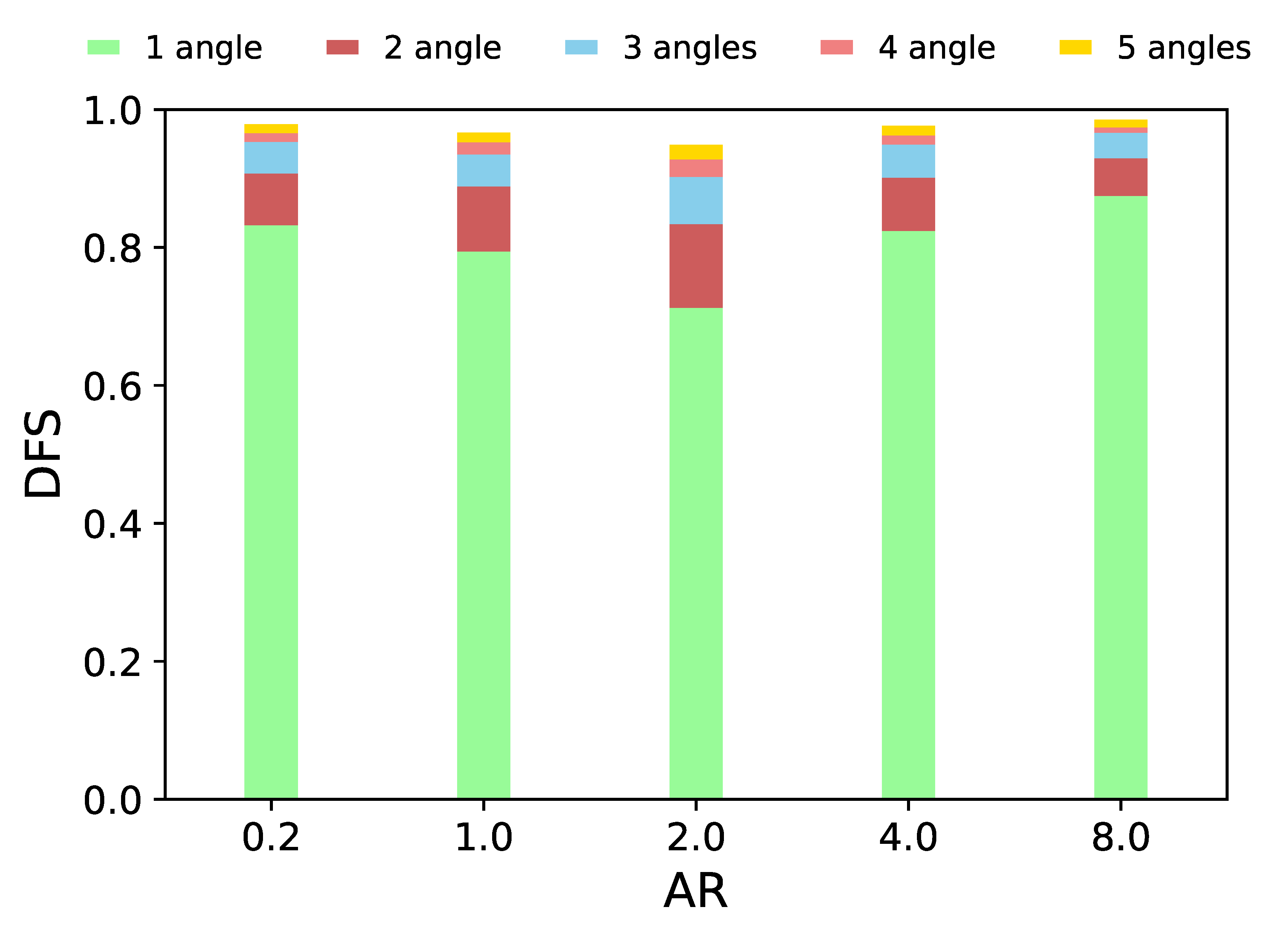
AR	0.2, 1.0, 2.0, 4.0, 8.0
σ *	0, 0.1, 0.2, 0.3, 0.4, 0.5
Re	1–90 µm
COT	>5

* σ is defined following Liu et al. [54] and Yang et al. [55], and larger values of σ indicate more severe surface roughness.

summarizes the cloud property parameters used in this study.

Ice cloud particle is assumed to be solid hexagonal columns or plates, i.e., the most widely used option for remote sensing and radiative transfer models of ice clouds [56]. The improved geometric-optics method (IGOM) is used to calculate the scattering properties for the assumed ice cloud particles [56,57]. The bulk scattering properties are calculated by averaging over the gamma size distribution with an effective variance of 0.1.

The six independent nonzero elements of the scattering matrix (P₁₁, P₁₂, P₂₂, P₃₃, P₄₃, and P₄₄), determined by the ice cloud particle model and validated by comparing with the results of previous studies, e.g., [5,54,58], are the essential variables used in the RT model to simulate the TOA intensity and polarization observations. Figure 1 compares the scattering matrix elements (P₁₁ and −P₁₂/P₁₁) of solid hexagonal columns with different σ (a-b) and ARs (c-d). Figure 1a,b (top panels) clearly illustrates the differences between the smooth and rough particles. As expected, the P₁₁ of smooth particle shows obvious oscillations, while it becomes smooth for rough particles [54]. The P₁₁ of rough particles with the same AR show less variations, while there are slight differences among their −P₁₂/P₁₁ (see Figure 1b). From the bottom panels, it is worth noting that the P₁₁ of the particles with ARs of 0.2 and 4 are similar while their −P₁₂/P₁₁ show obvious differences (black and green curves in Figure 1c,d). This means that polarization observations have the potential to distinguish ice particle habits (i.e., hexagonal particles with different AR or σ), which is consistent with the findings of [58,59].

3. Results

This study considers five channels centered at the 0.87, 1.24, 1.38, 1.64 and 2.13 µm, which are the “popular” channels for cloud retrievals. The sensitivities of these five channels (from left to right) with respect to COT are analyzed in Figure 2. Simulations are performed for single-layer ice clouds with a COT of 5.5 at a solar zenith angle (SZA) of 40° to ensure the saturation of polarized radiation for thick clouds. The ice cloud particle model is assumed to be a solid hexagonal column with a R_e of 30 µm, a σ of 0.5 and an AR of 0.2. The simulated TOA intensity and polarization (characterizing polarized information with degrees of linear polarization DOLP, DOLP = −Q/I) observations and the corresponding Jacobians of COT are illustrated in Figure 2. The TOA intensities at 1.64 and 2.13 µm are relatively small, which results from the cloud absorptions in these channels. The intensities are larger at the viewing angles opposite to the incident direction than other directions due to the enhanced cloud scattering in the forward scattering region (Figure 1c and Figure 2a–e). The larger TOA DOLP around the forward and side scattering directions (Figure 2f–j) are caused by the larger −P₁₂/P₁₁ values at scattering angles between 60° and 140° (see Figure 1b). The Jacobians of TOA intensity and DOLP with respect to COT at different spectral channels are illustrated in Figure 2l–u; a larger Jacobian value indicates that the TOA intensity or DOLP is more sensitive to COT. For the intensity observations, COTs exhibit a different type of spectral sensitivity, i.e., larger Jacobians are noticed at the 0.87 µm channel. The Jacobians of TOA intensity gradually decrease with an increase in the viewing zenith angle (VZA) and show a weaker relative azimuthal angular (RAA) dependence. The magnitudes of the intensity Jacobians are mostly larger than the precision for intensity observation sensitivity (0.01), indicating the possibility of COT retrieval. The TOA DOLP decreases as COT increases at the viewing geometries opposite to the incident, i.e., the negative Jacobians in Figure 2q–u. The magnitudes of the DOLP Jacobians are mostly smaller than the precision of the polarization observations (0.001). In general, when COT is larger than 5, the TOA intensity shows a high sensitivity to COT, while the saturated DOLP cannot be used to infer COT. The magnitudes of the Jacobians differ among the retrieved cloud property parameters, leading to different sensitivities and IC/DFS in the retrievals. The IC/DFS of other cloud properties will be discussed below.

Figure 3 shows the variations of total DFS as the number of measurement vector elements increase in a single-angle mode, and a larger DFS indicates a better estimation of ice cloud property parameters. We start from a measurement vector with two elements, i.e., the intensity at the 0.87 and 2.13 µm channels (I_0.87 and I_2.13, respectively), corresponding to the widely used two observations for the Nakajima–King method. Based on these two channels, we continue to calculate the DFS for three-element measurement vectors. From here on, either the intensity or the DOLP observation at a spectral channel is added as an additional measurement vector element to increase the DFS. Figure 3 adopts the names of the added elements as the x-axis. For example, the red curve gives the DFS with three elements, i.e., the original two and the added element indicated by the x-axis, and a maximum of seven elements are considered. For each addition, the best additional element/observation can be defined as the one that gives the largest DFS, e.g., DOLP_2.13 is the first best addition at R_e = 15 µm. Then, the best addition is defined as the third element, and we will perform the four-element tests. The black curve indicates the DFS of a four-element measurement vector, from which the second-best addition can be found. Repeat the similar processes, and the optimal combination of multi-spectral and multi-polarization observations can be found.

For small-sized particles with the R_e of 15 µm (left panel of Figure 3), adding polarization observations to the measurement vector significantly increases the DFS. From the red curve, the first-best addition is the polarization observation at the 2.13 µm channel (DOLP_2.13), as the DFS can increase from less than 2.0 to greater than 2.7. The second- and third-best additions with the highest DFS from the black and blue curves can be found as the intensity and polarization observations at the 1.64 µm channel (I_1.64 and DOLP_1.64). The fourth-best addition is the polarization observation at the 0.87 µm channel (DOLP_0.87). The DFS differences by adding the fourth-best addition are really small, and adding the fifth-best addition (to a total of 7) results in little improvement in DFS. In other words, DFS of the six-element measurement vector is considered close to saturation. Now, we consider medium-sized particles with the R_e of 30 µm (the middle panel). The first-best addition is the intensity observation at the 1.24 µm channel (I_1.24), and the second- and third-best additions are the polarization observations at the 0.87 and 2.13 µm channels (DOLP_0.87 and DOLP_2.13), respectively, while the fourth-best one is the intensity observation at the 1.64 µm channel (I_1.64). Repeating the same analysis, the optimal additional observations for large-sized particles with the R_e of 45 µm are DOLP_2.13, I_1.24, DOLP_0.87, and DOLP_1.24 (the right panel). Comparing the three panels in Figure 3 clearly shows that adding more multi-spectral and multi-polarization information would significantly benefit retrievals of small-sized particles, while having less influence on the retrievals of large-sized particles.

The improvement in total DFS is achieved mainly by the addition of the first- and second-best additions to the two-element measurement vector, and the difference in DFS becomes less significant by including more observations. Considering the different sizes of ice cloud particles, for the six-element measurement vector, the optimal observation combination is found to be I_0.87, I_2.13, I_1.24, DOLP_0.87, DOLP_2.13 and I_1.64. From here on, all simulations and discussions are based on five cases of two- to six-element measurement vectors, as listed in

Table 2. The multi-spectral and multi-polarization observation combinations.

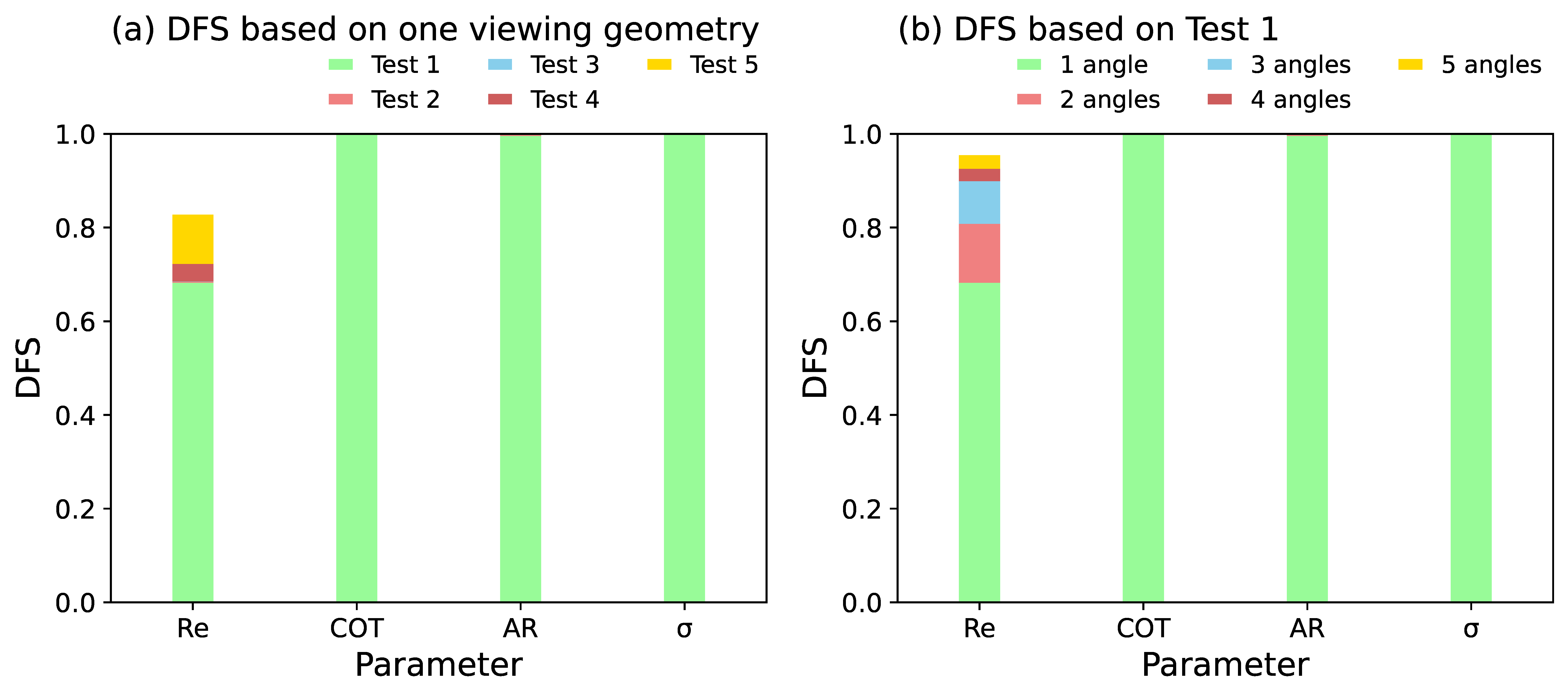
Test	Observation Combination
1	I0.87, I2.13
2	I0.87, I2.13, I1.24
3	I0.87, I2.13, I1.24, DOLP0.87
4	I0.87, I2.13, I1.24, DOLP0.87, DOLP2.13
5	I0.87, I2.13, I1.24, DOLP0.87, DOLP2.13, I1.64

.

4. Discussions

Figure 3 shows that the use of an optimal observation combination (Test 5) improves the total DFS of the four cloud property parameters, especially for small-sized ice cloud particles. The impact of adding multi-angle observations is illustrated in Figure 4 (Figure 4a for medium-sized ice cloud particles and Figure 4b for small-sized particles). For Test 1 (I_0.87 and I_2.13), the DFS in multi-angle mode increases significantly by ~1.6 compared to that in single-angle mode. Although the optimal observation combination provides considerable DFS in single-angle mode, the improvement is also obvious with the additional information from multi-angle observations. For the optimal observation combination (Test 5), once the number of multi-angle observations reaches three, the DFS becomes almost saturated and will not significantly improve by adding observations from other viewing geometries. Moreover, the DFS for Test 5 in single-angle mode is about 2.3 while that for Test 1 in 5-angle mode can rise as high as 3.6. This phenomenon indicates that the improvement of the DFS achieved by including multi-angle observations is more obvious than that achieved by including multi-spectral and multi-polarization observations. The same analyses and discussions for small-sized particles (R_e = 15µm) are carried out and shown in Figure 4b. The additional polarization observations can increase the total DFS effectively, while the additional intensity observations have less or no effect. For small-sized particles, the DFS in three-angle mode is close to saturation regardless of the changes of observation combination. In summary, ice cloud properties can be better retrieved by using the optimal observation combination from three viewing geometries, and additional angular variations will be less meaningful for such retrievals.

The above discussions focus on the total DFS of the four cloud property parameters (R_e, COT, AR and σ). Figure 5a shows the DFS of each cloud parameter associated with different observation combinations in single-angle mode for ice cloud particles with a R_e of 30 µm. The improvement of DFS is most obvious for R_e as the DFS increases from 0.68 in Test 1 to more than 0.82 in Test 5. The improvements of R_e DFS with the additional information from I_1.64 and DOLP_2.13 are obvious, while those from I_1.24 and DOLP_0.87 are too small to be noticed. This is consistent with the fact that the cloud absorption channels are more sensitive to R_e, as the TOA radiance decreases with the increase in R_e in these channels. Figure 5b shows the DFS for each cloud parameter associated with different viewing geometries for Test 1 (I_0.87 and I_2.13). Similarly, the additional information acquired in multi-angle mode is most significant for R_e with DFS increasing from 0.68 in single-angle mode to over 0.95 in multi-angle mode. This may be explained by the fact that the information of R_e is different at different viewing geometries, consequently, the R_e DFS increases with additional information from multi-angle observations. The comparison between the R_e DFS of Figure 5a,b is consistent with the aforementioned discussion that adding multi-angle observations can result in a better increase in the DFS of R_e. For ice particles with the R_e of 15 µm, the increases in R_e DFS also dominate the increase in the total DFS (Figures not shown). Overall, R_e has considerable uncertainties, but the use of multi-spectral, -angle and -polarization observations may be able to reduce the uncertainties and improve the accuracy of R_e retrievals. For other parameters, as a large amount of information can be obtained in single-angle mode, the improvement of DFS in multi-angle mode is not obvious. It is worth noting that, for Test 1 in single-angle mode, the sum of the four DFS pertaining to each of the cloud property parameters is ~3.67, while the total DFS considering the four parameters simultaneously is only 1.98. Similarly, the sum of the four DFS of each parameter is not exactly the same as the total DFS no matter how the combination of observations or viewing geometries change. This may be due to overlapping information, as AR and σ are all microphysics properties to influence optical properties and they cannot be characterized well by DFS.

We investigate the R_e DFS in more details. The angular distributions of the R_e DFS with different observation combinations in single-angle mode are shown in Figure 6. Consistent with the finding reached from Figure 5, adding I_1.64 and DOLP_2.13 is the key to increase the R_e DFS. When DOLP at the 2.13 µm channel is included (Test 4), the improvement of the DFS is observed mainly at viewing angles opposite to the solar incident (Figure 6d). This is owing to the larger DOLP Jacobians near these angles (Figure 6p). The same analysis can be applied to the increase in the R_e DFS around the backscattering directions when adding observation of I_1.64 in Test 5 (Figure 6e,j). In summary, the improvements in R_e DFS with the addition of multiple intensity or DOLP observations are consistent with their larger intensity or DOLP Jacobians with respect to R_e.

In Figure 7, we select ice cloud particles with different ARs and calculate the R_e DFS using an optimal observation combination (Test 5). The above discussions show that DFS in 3-angle mode is almost saturated and can be used to retrieve ice cloud properties. The ice cloud particle with the most obvious improvement of the R_e DFS is the particle with an AR of 2.0, where its P₁₁ changes most in the first three viewing geometries. In contrast, the result for the particle with an AR of 8.0 is the opposite, where P₁₁ changes are smallest. This confirms the consistent relationship between the changes of P₁₁ and the improvements of R_e DFS. The difference in the DFS between ice cloud particles is related to their scattering properties, and the use of multi-angle observations can improve DFS.

Figure 8 shows the angular distributions of the TOA intensity and DOLP for particles with different σ (1a–1j for smooth particles and 2a–2j for severely rough particles). The angular distributions of the TOA intensity and DOLP for smooth and rough particles are similar, but there are significant differences in their values, and the relative differences between these particles are shown in Figure 8(3a–3j). The relative differences in the intensity at cloud-absorbing channels are larger as the intensities are relatively small, and shows an obvious angular dependence with smaller differences around the directions close to the incoming beam and the viewing geometries opposite to the incident direction (Figure 8(3a–3e)). In contrast, the relative difference in the TOA DOLP demonstrate a complex angular distribution: the larger differences occur around the backscattering directions, and the largest difference occurs at the viewing geometry with a VZA of 40° and an RAA of 160°, which corresponds to a scattering angle of 120°. This can be explained by the fact that the scattering matrix element −P₁₂/P₁₁ of the smooth and rough particles have the largest difference at these scattering angles (120°). Similarly, the difference in the peak with the scattering angle of 60° at the 2.13 µm channel corresponds to the largest difference with the VZA of 70° and RAA of 120° (Figure 8(3j)). The DOLP relative differences are larger than those of the intensity, indicating that polarization observations are more sensitive to these differences and can provide the potential for retrieving particle surface roughness level if other variables are well and accurately known. Furthermore, we also test the angular differences due to different hexagonal habits. The results for particles with different ARs but the same roughness variable are also closely related to their differences on the scattering phase matrix elements, and we will not discuss them in details.

Figure 9 demonstrates the total DFS of four cloud property parameters (R_e, COT, AR, σ) for particles with different sizes, where R_e is in the range from 1 to 90 µm. Adding either multi-angle or multi-spectral and multi-polarization observations plays a key role in the improvement in the total DFS. In addition, the improvement in the DFS achieved by adding polarization observations (i.e., DOLP_0.87 and DOLP_2.13) is more obvious when R_e is in the range from 1 to 20 µm, as polarization observations are more sensitive to small-sized particles than to larger-sized particles, which is consistent with the previous results. For most particles, the improved DFS from the additional multi-angle observations is more obvious than that from the additional multi-spectral and multi-polarization observations, which can be seen from a comparison of the DFS of Test 5 in single-angle mode with the DFS of Test 1 in 5-angle mode.

According to the discussion in this section, the polarization observations have the potential to distinguish particle habits (defined by AR and σ), whereas this is based on well-known other variables. The use of multi-spectral, -angle, and -polarization observations, especially the optimal observation combination from three viewing geometries, plays an important role in improving DFS/IC. The increased DFS of cloud properties indicates that more information can be obtained from observations or the ice cloud properties can be retrieved more accurately. Among the four parameters considered, R_e introduces larger uncertainties, which may be reduced by the employment of multi-spectral, -angle and -polarization observations. The improvements in the R_e DFS correspond to the Jacobians with respect to R_e and the changes of particle scattering matrix elements (P₁₁ and −P₁₂/P₁₁) in viewing geometries. Our numerical results show that the total DFS improvement is mainly contributed by that related to R_e.

5. Conclusions

This study investigates the potential of multi-spectral, -angle and -polarization observations to better retrieve ice cloud properties based on simulated results and information content (IC) analysis. An accurate polarized radiative transfer model comprising cloud scattering is used to simulate the top-of-atmosphere (TOA) intensity and polarization observations. The ice cloud particle model is assumed to be the solid hexagonal column habit, and the considered cloud properties are particle effective radius (R_e), aspect ratio (AR), surface roughness level (σ) and cloud optical thickness (COT). The Jacobians of the intensity and polarization observations at TOA with respect to different ice cloud property parameters (i.e., COT and R_e) at different viewing geometries are discussed. The effects of multi-spectral, -angle and -polarization observations on ice cloud property retrievals specified by DFS are analyzed with different observation combinations and viewing geometries. The conclusions of this study can benefit the design of future multi-spectral, -angle and –polarization instruments.

There is no doubt the ice cloud property retrievals can be improved with the additional information from multi-spectral, -angle and -polarization observations, which is verified by the increased DFS. Considering different spectral and polarized channels, the optimal observation combination is found to be I_0.87, I_2.13, I_1.24, DOLP_0.87, DOLP_2.13, and I_1.64. Polarization observations are more sensitive to small-sized particles than to larger-sized particles and small-sized particles have a greater DFS than large-sized ones. The total DFS of four cloud property parameters can be significantly increased with the additional information from the optimal observation combination at multiple viewing geometries. Compared with the result in multi-spectral and multi-polarization mode, the improvement of the total DFS acquired in multi-angle mode is more significant, i.e., from ~1.9 to ~3.6, by considering observations from different viewing geometries. Moreover, the multi-angle and -polarization observations can hardly further improve the retrieval of COT. This is owing to the saturated polarization when COT is larger than ~5, and the weaker angular dependence of intensity Jacobians with known particle habits. Polarization observations have the potential to reveal the ice cloud particle habits (defined by AR and σ), whereas particle habit signals may be overlapped can hardly be separated nor characterized. Among the four property parameters considered, the R_e retrievals exhibit larger uncertainties, and the uncertainties can be reduced by using multi-spectral, -angle and -polarization observations. Both the total DFS and the DFS of R_e become saturated regardless of the changes in multi-spectral and multi-polarization observation combinations when considering the observations from three viewing geometries. It is worth noting that only the observational uncertainties are considered in our IC analyses. If other errors, such as those from retrievals or model assumptions (e.g., particle optical properties, forward radiative transfer and cloud height assumption) were taken into consideration, error-corrected observations may be used to better understand their influences on cloud property retrievals.

In brief, it is recommended to use the observations composing the optimal observation combination from three viewing geometries to retrieve ice cloud properties to improve the retrieval performance. The conclusions obtained from this study have the potential to provide a theoretical foundation for developing a cloud property retrieval algorithm with the use of multi-spectral, -angle and -polarization observations. Last but not least, this study uses idealized numerical models and simulations to provide a fundamental analysis of the information content of ice cloud properties, and such discussions with actual satellite observations will be investigated in further studies.

References

- Nazaryan, H.; McCormick, M.P.; Menzel, W.P. Global characterization of cirrus clouds using CALIPSO data. J. Geophys. Res. 2008, 113, D16211. [Google Scholar] [CrossRef]
- Baker, M.B.; Peter, T. Small-scale cloud processes and climate. Nature 2008, 451, 299–300. [Google Scholar] [CrossRef] [PubMed]
- Liou, K.N.; Yang, P. Light Scattering by Ice Crystals: Fundamentals and Applications; Cambridge University Press: Cambridge, UK, 2016. [Google Scholar]
- Chepfer, H.; Brogniez, G.; Fouquart, Y. Cirrus clouds’ microphysical properties deduced from POLDER observations. J. Quant. Spectrosc. Radiat. Transf. 1998, 60, 375–390. [Google Scholar] [CrossRef]
- Saito, M.; Iwabuchi, H.; Yang, P.; Tang, G.; King, M.D.; Sekiguchi, M. Ice particle morphology and microphysical properties of cirrus clouds inferred from combined CALIOP-IIR measurements. J. Geophys. Res. Atmos. 2017, 122, 4440–4462. [Google Scholar] [CrossRef]
- Lai, R.; Teng, S.; Yi, B.; Letu, H.; Min, M.; Tang, S.; Liu, C. Comparison of clouds properties from Hamawari-8 and FengYun-4A geostationary satellite radiometers with MODIS cloud retrievals. Remote Sens. 2019, 11, 1703. [Google Scholar] [CrossRef] [Green Version]
- Wang, Y.; Su, H.; Jiang, J.H.; Xu, F.; Yung, Y.L. Impact of cloud ice particle size uncertainty in a climate model and implications for future satellite missions. J. Geophys. Res. 2020, 125, D032119. [Google Scholar]
- Kidd, C.; Levizzani, V.; Bauer, P. A review of satellite meteorology and climatology at the start of the twenty-first century. Prog. Phys. Geogr. 2009, 33, 474–489. [Google Scholar] [CrossRef]
- Zhao, L.; Zhao, C.; Wang, Y.; Yang, Y. Evaluation of cloud microphysical properties derived from MODIS and Himawari-8 using in situ aircraft measurements over the Southern Ocean. Earth Space Sci. 2020, 7, e2020EA001137. [Google Scholar] [CrossRef] [Green Version]
- King, M.D.; Platnick, S.; Menzel, W.P.; Ackerman, S.A.; Hubanks, P.A. Spatial and temporal distribution of clouds observed by MODIS onboard the Terra and Aqua satellites. IEEE Trans. Geosci. Remote Sens. 2013, 51, 3826–3852. [Google Scholar] [CrossRef]
- King, M.D.; Menzel, W.P.; Kaufman, Y.J.; Tanre, D.; Gao, B.-C.; Platnick, S.; Ackerman, S.; Remer, L.; Pincus, R.; Hubanks, P. Cloud and aerosol properties, precipitable water, and profiles of temperature and water vapor from MODIS. IEEE Trans. Geosci. Remote Sens. 2003, 41, 442–458. [Google Scholar] [CrossRef] [Green Version]
- Hsu, N.C.; Lee, J.; Sayer, A.M.; Carletta, N.; Chen, S.H.; Tucker, C.J.; Holben, B.N.; Tsay, S.C. Retrieving near-global aerosol loading over land and ocean from AVHRR. J. Geophys. Res. Atmos. 2017, 122, 9968–9989. [Google Scholar] [CrossRef] [Green Version]
- Parol, F.; Buriez, J.C.; Brogniez, G.; Fouquart, Y. Information content of AVHRR Channels 4 and 5 with respect to the effective radius of Cirrus Cloud particles. J. Appl. Meteorol. 1991, 30, 973–984. [Google Scholar] [CrossRef]
- Yang, J.; Zhang, Z.; Wei, C.; Lu, F.; Guo, Q. Introducing the new generation of Chinese geostationary weather satellites-FengYun 4 (FY-4). Bull. Am. Meteorol. Soc. 2017, 98, 1637–1658. [Google Scholar] [CrossRef]
- Da, C. Preliminary assessment of the Advanced Himawari Imager (AHI) measurement onboard Himawari-8 geostationary satellite. Remote Sens. Lett. 2015, 6, 637–646. [Google Scholar] [CrossRef]
- Nakajima, T.; King, M.D. Determination of the optical thickness and effective particle radius of clouds from reflected solar radiation measurements. Part I: Theory. J. Atmos. Sci. 1990, 47, 1878–1893. [Google Scholar] [CrossRef] [Green Version]
- Platnick, S.; Meyer, K.; King, M.D.; Wind, G.; Amarasinghe, N.; Marchant, B.; Arnold, G.T.; Zhang, Z.; Hubanks, P.A.; Holz, R.E.; et al. The MODIS cloud optical and microphysical products: Collection 6 updates and examples from Terra and Aqua. IEEE Trans. Geosci. Remote Sens. 2017, 55, 502–525. [Google Scholar] [CrossRef] [Green Version]
- Marshak, A.; Platnick, S.; Várnai, T.; Wen, G.; Cahalan, R.F. Impact of three-dimensional radiative effects on satellite retrievals of cloud droplet sizes. J. Geophys. Res. 2006, 111, D09027. [Google Scholar] [CrossRef]
- Fu, D.; Girolamo, L.D.; Liang, L.; Zhao, G. Regional biases in Moderate Resolution Imaging Spectroradiometer (MODIS) marine liquid water cloud drop effective radius deduced through fusion with Multi-angle Imaging SpectroRadiometer (MISR). J. Geophys. Res. 2019, 124, 13182–13196. [Google Scholar]
- Ohring, G.; Wielicki, B.A.; Spencer, R.W.; Emery, B.; Datla, R.V. Satellite instrument calibration for measuring global climate change: Report of a workshop. Bull. Am. Meteorol. Soc. 2005, 86, 1303–1313. [Google Scholar] [CrossRef]
- Diner, D.J.; Bruegge, C.J.; Martonchik, J.V.; Ackerman, T.P.; Davies, R.; Gerstl, S.A.W.; Gordon, H.R.; Sellers, P.J.; Clark, J.; Daniels, J.A.; et al. MISR: A Multi-angle Imaging SpectroRadiometer for geophysical and climatological research from EOS. IEEE Trans. Geosci. Remote Sens. 1989, 27, 200–214. [Google Scholar] [CrossRef]
- Liang, L.; Girolamo, L.D. A global analysis on the view-angle dependence of plane-parallel oceanic liquid water cloud optical thickness using data synergy from MISR and MODIS. J. Geophys. Res. 2013, 118, 2389–2403. [Google Scholar] [CrossRef]
- Lee, B.; Girolamo, L.D.; Zhao, G.; Zhan, Y. Three-dimensional cloud volume reconstruction from the multi-angle Imaging SpectroRadiometer. Remote Sens. 2018, 10, 1858. [Google Scholar] [CrossRef] [Green Version]
- Bréon, F.M. Parasol Level-1 Product Data Format and User Manual; CNES: Paris, France, 2005; Available online: http://www.icare.univ-lille1.fr/parasol/?rubrique=overview_product (accessed on 5 August 2020).
- Deschamps, P.Y.; Bréon, F.; Leroy, M.; Bricaud, A.; Buriez, J.C.; Seze, G. The POLDER mission: Instrument characteristics and scientific objectives. IEEE Trans. Geosci. Remote Sens. 1994, 32, 598–615. [Google Scholar] [CrossRef]
- Parol, F.; Buriez, J.C.; Vanbauce, C.; Riedi, J.; Labonnote, L.C.; Doutriaux-Boucher, M.; Vesperini, M.; Seze, G.; Couvert, P.; Viollier, M.; et al. Review of capabilities of multi-angle and polarization cloud measurements from POLDER. Adv. Space Res. 2004, 33, 1080–1088. [Google Scholar] [CrossRef]
- Zheng, F.; Hou, W.; Li, Z. Optimal estimation retrieval for directional polarimetric camera onboard Chinese Gaofen-5 satellite: An analysis on multi-angle dependence and a posteriori error. Acta Phys. Sin. 2019, 68, 040701. [Google Scholar]
- Chen, F.; Huang, C.; Hong, J.; Luo, D.; Sun, L.; Sun, X.; Wei, W. In Flight Radiation evaluation and validation of Directional Polarimetric Camera. Aerosp. Shanghai 2019, 36, 126–136. [Google Scholar]
- Manolis, I.; Caron, J.; Grabarnik, S.; Bézy, J.L.; Betto, M.; Barrè, H.; Mason, G.; Meynart, R. The MetOp second generation 3MI mission. In Proceedings of the International Conference on Space Optics, Ajaccio, Corsica, France, 9–12 October 2012. Available online: https://doi.org/10.1117/12.2309178 (accessed on 5 August 2020).
- Girolamo, L.D.; Wilson, M.J. A first look at band-differenced angular signatures for cloud detection from MISR. IEEE Trans. Geosci. Remote Sens. 2003, 41, 1730–1734. [Google Scholar] [CrossRef]
- Buriez, J.C.; Vanbauce, C.; Parol, F.; Goloub, P.; Herman, M.; Bonnel, B.; Fouquart, Y.; Couvert, P.; Seze, G. Cloud detection and derivation of cloud properties from POLDER. Int. J. Remote Sens. 1997, 18, 2785–2813. [Google Scholar] [CrossRef]
- Yi, B.; Huang, X.; Yang, P.; Baum, B.A.; Kattawar, G.W. Considering polarization in MODIS-based cloud property retrievals by using a vector radiative transfer code. J. Quant. Spectrosc. Radiat. Transf. 2014, 146, 540–548. [Google Scholar] [CrossRef]
- Goloub, P.; Deuze, J.L.; Herman, M.; Fouquart, Y. Analysis of the POLDER polarization measurements performed over cloud covers. IEEE Trans. Geosci. Remote Sens. 1994, 32, 78–88. [Google Scholar] [CrossRef]
- van Diedenhoven, B.; Cairns, B.; Geogdzhayev, I.V.; Fridlind, A.M.; Ackerman, A.S.; Yang, P.; Baum, B.A. Remote sensing of ice crystal asymmetry parameter using multi-directional polarization measurements-Part 1: Methodology and evaluation with simulated measurements. Atmos. Meas. Tech. 2012, 5, 2361–2374. [Google Scholar] [CrossRef] [Green Version]
- Cole, B.H.; Yang, P.; Baum, B.A.; Riedi, J.; Labonnote, L.C.; Thieuleux, F.; Platnick, S. Comparison of PARASOL observations with polarized reflectances simulated using different ice habit mixtures. J. Appl. Meteorol. Climatol. 2013, 52, 186–196. [Google Scholar] [CrossRef]
- Chepfer, H.; Goloub, P.; Riedi, J.; De Haan, J.F.; Hovenier, J.W.; Flamant, P.H. Ice crystal shapes in cirrus clouds derived from POLDER-1/ADEOS-1. J. Geophys. Res. 2001, 106, 7955–7966. [Google Scholar] [CrossRef] [Green Version]
- Cole, B.H.; Yang, P.; Baum, B.A.; Riedi, J.; Labonnote, L.C. Ice particle habit and surface roughness derived from PARASOL polarization measurements. Atmos. Chem. Phys. 2013, 14, 3739–3750. [Google Scholar] [CrossRef] [Green Version]
- Hioki, S.; Yang, P.; Baum, B.A.; Platnick, S.; Meyer, K.; King, M.D.; Riedi, J. Degree of ice particle surface roughness inferred from polarimetric observations. Atmos. Chem. Phys. 2015, 16, 7545–7558. [Google Scholar] [CrossRef] [Green Version]
- Shang, H.; Chen, L.; Bréon, F.M.; Letu, H.; Li, S.; Wang, Z.; Su, L. Impact of cloud horizontal inhomogeneity and directional sampling on the retrieval of cloud droplet size by the POLDER instrument. Atmos. Meas. Tech. 2015, 8, 4931–4945. [Google Scholar] [CrossRef] [Green Version]
- Shang, H.; Letu, H.; Bréon, F.M.; Riedi, J.; Ma, R.; Wang, Z.; Nakajima, T.Y.; Wang, Z.; Chen, L. An Improved Algorithm of Cloud Droplet Size Distribution from POLDER Polarized Measurements. Remote Sens. Environ. 2019, 228, 61–74. [Google Scholar] [CrossRef]
- Masuda, K.; Ishimoto, H.; Takashima, T. Retrieval of cirrus optical thickness and ice-shape information using total and polarized reflectance from satellite measurements. J. Quant. Spectrosc. Radiat. Transf. 2002, 1, 39–51. [Google Scholar] [CrossRef]
- Chen, X.; Wang, J.; Liu, Y.; Xu, X.; Cai, Z.; Yang, D.; Yan, C.-X.; Feng, L. Angular dependence of aerosol information content in CAPI/TanSat observation over land: Effect of polarization and synergy with A-train satellites. Remote Sens. Environ. 2017, 196, 163–177. [Google Scholar] [CrossRef]
- Chen, X.; Yang, D.; Cai, Z.; Liu, Y.; Spurr, R. Aerosol retrieval sensitivity and error analysis for the cloud and aerosol polarimetric imager on board TanSat: The effect of multi-angle measurement. Remote Sens. 2017, 9, 183. [Google Scholar] [CrossRef] [Green Version]
- Huang, X.; Yang, P.; Kattawar, G.W.; Liou, K.N. Effect of mineral dust aerosol aspect ratio on polarized reflectance. J. Quant. Spectrosc. Radiat. Transf. 2015, 151, 97–109. [Google Scholar] [CrossRef]
- Rodgers, C.D. Inverse Methods for Atmospheric Sounding: Theory and Practice; World Scientific: Singapore, 2000. [Google Scholar]
- Wang, C.; Platnick, S.; Zhang, Z.; Meyer, K.; Yang, P. Retrieval of ice cloud properties using an optimal estimation algorithm and MODIS infrared observations: 1. Forward model, error analysis, and information content. J. Geophys. Res. Atmos. 2016, 121, 5809–5826. [Google Scholar] [CrossRef] [PubMed] [Green Version]
- Li, Z.; Blarel, L.; Podvin, T.; Goloub, P.; Chen, L. Calibration of the degree of linear polarization measurement of polarized radiometer using solar light. Opt. Soc. Am. 2010, 49, 1249–1256. [Google Scholar] [CrossRef] [PubMed]
- Xu, X.; Wang, J. Retrieval of aerosol microphysical properties from AERONET photopolarimetric measurements: Q. Information content analysis. J. Geophys. Res. Atmos. 2015, 120, 7059–7078. [Google Scholar] [CrossRef] [Green Version]
- Sun, W.; Loeb, N.G.; Yang, P. On the retrieval of ice cloud particle shapes from POLDER measurements. J. Quant. Spectrosc. Radiat. Transf. 2006, 101, 435–447. [Google Scholar] [CrossRef]
- De Haan, J.F.; Bosma, P.B.; Hovenier, J.W. The adding method for multiple scattering calculations of polarized light. Astron. Phys. 1987, 183, 371–391. [Google Scholar]
- Tomasi, C.; Vitale, V.; Petkov, B.; Lupi, A.; Cacciari, A. Improved algorithm for calculations of Rayleigh scattering optical depth in standard atmosphere. Appl. Opt. 2005, 44, 3320–3341. [Google Scholar] [CrossRef]
- Duan, M.; Min, Q.; Lu, D. A polarized radiative transfer model based on successive order of Scattering. Adv. Atmos. Sci. 2010, 27, 891–900. [Google Scholar] [CrossRef]
- Wang, C.; Platnick, S.; Zhang, Z.; Meyer, K.; Wind, G.; Yang, P. Retrieval of ice cloud properties using an optimal estimation algorithm and MODIS infrared observations: 2. Retrieval evaluation. J. Geophys. Res. Atmos. 2016, 121, 5827–5845. [Google Scholar] [CrossRef]
- Liu, C.; Panetta, R.L.; Yang, P. The effects of surface roughness on the scattering properties with sizes from the Rayleigh to the geometric-optics regimes. J. Quant. Spectrosc. Radiat. Transf. 2013, 129, 169–185. [Google Scholar] [CrossRef]
- Yang, P.; Bi, L.; Baum, B.A.; Liou, K.N.; Kattawar, G.W.; Mishchenko, M.I.; Cole, B.H. Spectrally consistent scattering, absorption, and polarization properties of atmospheric ice crystals at wavelengths from 0.2 to 100 μm. J. Atmos. Sci. 2013, 70, 330–347. [Google Scholar] [CrossRef]
- Liu, C.; Panetta, R.L.; Yang, P.; Macke, A.; Baran, A.J. Modeling the scattering properties of mineral aerosols using concave fractal polyhedral. Appl. Opt. 2013, 52, 640–652. [Google Scholar] [CrossRef] [PubMed]
- Yang, P.; Liou, K.N. Single-scattering properties of complex ice crystals in terrestrial atmosphere. Contrib. Atmos. Phys. 1998, 71, 223–248. [Google Scholar]
- Baum, B.A.; Yang, P.; Heymsfield, A.J.; Bansemer, A.; Cole, B.H.; Merrelli, A.; Schmitt, C.; Wang, C. Ice cloud single-scattering property models with the full phase matrix at wave lengths from 0.2 to 100 μm. J. Quant. Spectrosc. Radiat. Transf. 2014, 146, 123–139. [Google Scholar] [CrossRef]
- Lawless, R.; Xie, Y.; Yang, P.; Kattawar, G.W.; Laszlo, I. Polarization and effective Mueller matrix for multiple scattering of light by nonspherical ice crystals. Opt. Express 2006, 14, 6381–6393. [Google Scholar] [CrossRef]