Article

Wildfire Trend Analysis over the Contiguous United States Using Remote Sensing Observations

1
Department of Geosciences and Environment, California State University—Los Angeles, Los Angeles, CA 90032, USA
2
NASA Jet Propulsion Laboratory, California Institute of Technology, Pasadena, CA 91109, USA
*
Author to whom correspondence should be addressed.
Remote Sens. 2020, 12(16), 2565; https://doi.org/10.3390/rs12162565
Submission received: 27 June 2020 / Revised: 1 August 2020 / Accepted: 5 August 2020 / Published: 10 August 2020
(This article belongs to the Section Environmental Remote Sensing)

Abstract

:
Understanding the evolution of wildfire regimes throughout the United States (US) is crucial in the preparation, mitigation, and planning for national wildfires. Recent wildfire trajectories demonstrating an increase in both frequency and size across the US have made documenting the changes in wildfire regimes a topic of growing importance. While previous studies have examined wildfire regimes using ecoregions, this study analyzes wildfire regimes through the Geographic Area Coordination Center (GACC) regions across the Contiguous US over 34 years, 1984–2017. GACCs are geopolitical boundaries designed by wildfire agencies to promote an efficient way to distribute resources during emergencies such as wildfires. Wildfire observations originate from the Monitoring Trends in Burn Severity (MTBS) database which records large fire events that are 1000(500) acres or greater in the Western (Eastern) US. Using GACCs and MTBS data, this study examines wildfire regimes across the Contiguous US through the following three parameters: total burned area, frequency, and average burned area. This study characterizes the trend direction of the wildfire parameters and which are statistically significant. Results demonstrate that most GACC regions display statistically significant trends, including wildfire regimes that are beyond the Western US (e.g., Southern GACC). The Northwest and Southwest GACCs demonstrate statistically significant positive trends in every parameter observed. The California and Great Basin GACCs demonstrate statistically significant positive trends in the average burned area. The Eastern GACC is the only region to not display any significant trends. Determining significant wildfire regimes and their trend direction can help wildfire agencies to minimize the negative impacts on the environment, society, and economy.

Graphical Abstract

1. Introduction

Record-breaking fire seasons across the United States (US) have motivated policymakers, managers, and communities to develop new systems to better mitigate wildfires; a result of the expeditiously changing role of wildfires in social-ecological systems [1]. There is a growing awareness of the detrimental effects of wildfires on biodiversity, human health, and the economy [2]. The US Department of Agriculture-Forest Service has predicted that the economic cost of fire suppression would reach heights of nearly USD 1.8 billion per year [3]. The rising costs of fire suppression are making understanding wildfire regimes imperative. Additionally, changes in wildfire regimes are key to understand because wildfires are an integral part of Earth System processes that link and affect biogeochemical cycles, human activities, and vegetation patterns [4]. Ultimately, there is a growing need to comprehend the evolution of wildfires in the US at timescales of natural resources management.
This study quantifies historical fire trends across the Contiguous US (CONUS) in the context of Geographic Area Coordination Centers (GACC). GACCs are geopolitical boundaries with similar fire-weather types that have been outlined by a series of fire management organizations [5]. There are nine GACC regions across CONUS that define our wildfire regimes (see Section 2.2). Using this level of aggregation defined by fire management organizations is crucial for risk management because fire managers need to understand where wildfire hotspots exist, so fire suppression is implemented appropriately to protect resource values (e.g., infrastructure) and enhance ecosystem values [6]. In addition, this study uses GACC regions because climate–wildfire relationships at the GACC level is how climate information is expounded by fire management operations for seasonal planning, resource allocation (e.g., people, aircraft, equipment), financial support requests from Congress, and suppression activity [7]. Understanding wildfire regimes at the GACC level provides the necessary information for decision-makers at the national level where fiduciary planning and suppression resource allocation occurs [7]. In addition, as a result of the interagency collaboration within each GACC region, some GACCs have support programs in place for predictive services which is primarily monitoring weather and fuel conditions, and producing fire-weather related products [8]. One study used GACCs as a framework to assess the effectiveness of prescribed fires in the US [9]. Another study focused on four GACC regions in the Western US to analyze the fire frequency, burned area, and burn severity trends using Monitoring Trends in Burn Severity (MTBS) data [5]. Another study developed regression models specific to a GACC with the incorporation of input data such as vapor pressure deficit, soil moisture, other remote sensing fire data (e.g., Global Fire Emissions Database), and land cover data [10]. Results show how dynamic wildfire regimes are in relevance to one another, and regression models specific to a GACC can be used to predict area burned [10]. Therefore, GACCs is a useful tool for wildfire research.
The recent metamorphic changes in wildfires across the US have both natural and anthropogenic drivers. A study mentions that natural drivers such as temperature, precipitation, wind, and atmospheric moisture, are important factors in wildfire activity [11]. According to [11], temperature is the most essential element in increasing fire activity due to increasing evapotranspiration rates, increasing lighting activity (a type of ignition source), and lengthening the fire season. Another study demonstrated the effects of atmospheric rivers (a meteorological phenomenon for water transport from the tropics to midlatitude) in the enhancement of vegetation productivity and fuel loading—a critical aspect for moisture limited wildfire regimes [12]. Other studies have also demonstrated the connection between hydrological indicators and fire activity [13,14]. At a regional scale, the Western US deserts are projected to have conditions that increase the potential for wildfires because of increased invasive grass species in the region; this is likely facilitated by natural cycles of climate variability but can also be an influence from anthropogenic climate change [15]. Furthermore, nonnative grass species in the Southwestern US would make it more conducive for wildfires to occur in desert ecosystems which have been historically low [16]. Whereas in the Eastern US, defined as east of 100°W in CONUS, the probability for large wildfires increase when long-term drought, low fuel moisture, and elevated fire-weather align [17]. The aspect of climate–wildfire relationships has also been explored which depict that area burned and frequency in the Western US have increased over time [18,19]. Soil moisture conditions that are an antecedent to a fire-season also impact the frequency of large wildfire events depending on the land cover type [20]. A study assessed regional wildfire trends in the Western US and with additional analyses using climate information (e.g., temperature, precipitation), suggested that climate is a dominant driver for wildfire activity in the area [21].
Natural drivers of wildfire activity are an important facet, but anthropogenic drivers have also played a significant role. Human-caused large fire season is vastly longer than the lighting-caused large fire season in both the Eastern and Western portions of the US [22]. Human-ignited wildfires affect regions seasonally, most notably in the spring in the Eastern US and the fall and winter in Texas and Gulf states [23]. According to [24], large wildfires across the US are projected to increase and would likely be exacerbated by anthropogenic climate change. Hence, it is important to note that alterations of wildfire regimes have been dominantly driven by human influences through lengthening the fire season, increasing ignitions, and changing fuel availability throughout the US [23]. Anthropogenic climate change has also influenced fuel aridity (increasing flammability) in the Western US through increases in temperature and vapor pressure deficit trends [25]. Additionally, areas dominated by human ignitions exemplify fires that are two times more frequent and occur over fire season lengths that are 2.4 times longer [26]. However, areas dominated by lighting ignitions experience average fires that are increasing 23 times faster in size over time than areas dominated by anthropogenic activities [26]. In addition, the highest absolute gains in the wildland–urban interface (a region where housing and wildland vegetation interact) area occurred in the east; whereas, high gains in houses and people in the wildland–urban interface were most common in the South and Southwest portion of the US [27]. This is an important realization because humans are a crucial ignition source for wildfire activity.
Recognizing the formative influences of natural and anthropogenic drivers in wildfire activity this study conducts a statistical analysis on the total burned area, frequency, and average burned area trends across CONUS from 1984–2017. Statistical analysis of wildfire regimes has been a crucial element of national wildfire planning, operations, and research in the US. Historical analysis of wildfire activity contributes to many realms of research whether it be national fire danger rating applications, fire-potential forecast models, and geospatial fire modeling systems [28]. More importantly, spatiotemporal analyses of US wildfire regimes have gradually become intrinsic in the characterization of local, regional, and national patterns and trends since it can be related to a myriad of factors such as climate, population, land use, fire policy, and to predict how wildfire activity may be affected by such factors [28]. There is much value in understanding historical wildfire trends to characterize wildfire regimes. For example, the total burned area parameter provides an important aspect of the evolution of the GACC wildfire regimes. Understanding the frequency of large wildfires is also crucial because the relationship between frequency and time can serve as a good metric for predicting wildfires [29]. Furthermore, the average burned area trend is key to understand and can prove to be useful in developing better fire spread and behavior models.
This study uses wildfire data derived from remote sensing observations. Remote sensing observations, available since the 1980s, have revealed the global scope of wildfires and their impact; making it a valuable tool in gaining a better understanding of wildfire trends and regimes. Remote sensing techniques are capable of producing biophysical measurements of ground conditions both pre- and post-fire, which have been used to assist in fire risk mapping, fuel mapping, active fire detection, burned area estimates, assessments of burn severity, and for monitoring vegetation recovery [30]. For example, monitoring vegetation recovery using satellite observations aided in understanding the timing of vegetation greenness patterns during the first year after wildfires occurred [31], providing the approximate timing for ecological or geomorphic processes to return to pre-disturbance conditions in the rangelands of the Western US [31]. Another application of satellite observation has been used in conjunction with wildland fire models to simulate the growth of large wildfires [32]. Essentially for fire ecology research, remote sensing systems have been largely implemented because of their ability to provide images of the Earth at regular intervals and information on the amount of energy reflected in multiple regions of the electromagnetic spectrum [30].
MTBS data used in this study is one of the longest remote sensing observational records available, currently from 1984 to 2017, containing information on fire occurrences, burn severity, burn acreage, other geospatial information, and various other reports designed for use at local, state, and national levels [33]. The MTBS database is a well-established source for wildfire research. Various studies have implemented MTBS data with varying periods and study regions, to understand climate–wildfire relationships [7,17,24,34,35,36,37], analyze human influences on wildfire regimes [23,26,27,38], large wildfire trend identification within ecoregions [21,39], analyze the repercussions US wildfire management had on wildfire regimes [40], understand the role of how fuel treatments affect wildfire size and risk [41], and for the development of wildfire models to better predict large wildfire occurrences across the US [42]. However, some notable limitations of the MTBS database are that there is a ~2-year lag in the inclusion of data (limiting this study to 2017), islands of no detectable change are included in the derived fire perimeters, phenology offsets are not automatically applied to some spectral indices, and the existence of highly variable classification thresholds for mapping burn severity [43]. This study does not focus on the burn severity aspect of the MTBS database, but rather the perimeter data and associated trends (e.g., frequency). Despite limitations, these observations exist over a significant period which better accounts for variability in factors that can influence fire severity such as climate [33].
The importance of our study is that we disentangle which wildfire regimes are significant under the GACC premise across CONUS using the MTBS data. This would provide key information to fire managers, so they can better adapt, mitigate, and plan for national wildfires. This study characterizes wildfire regimes through the following three parameters from 1984 to 2017: total burned area, frequency, and average burned area. Each parameter per GACC has a corresponding linear regression (least-square method) and is tested for trend significance through the Mann–Kendall test to determine statistically significant wildfire parameters.

2. Materials and Methods

2.1. Wildfire Data

The MTBS project is a Wildland Fire Leadership Council, a national-level interagency body in charge of the National Fire Plan, sponsored project that incorporates the services of the US Geological Survey (USGS) and the US Department of Agriculture (USDA)-Forest Service [33]. The MTBS database provides data for this study which is designed to assess the environmental impacts of large wildland fires and pinpoint trends of fire severity on all lands across the US [33]. The USGS and USDA-Forest Service are the agencies responsible for setting the lower limit for what is classified as a large wildfire. The lower limits are a function of geographic location, all fires 1000 acres or greater in the continental US west of the 97° longitude, and 500 acres or greater east of the 97° longitude are incorporated in the MTBS database as large wildfires [21]. As previously mentioned, the strength of this database is the longevity which is an important factor to develop climate–fire relationships [33]. Another important advantage is that geospatial products, such as burn area boundaries, are derived under the same methodology that incorporates the Normalized Burn Ratio (NBR), which lessens the vulnerability of the data due to temporal and spatial variability in the fire reporting method [21].
The source of the MTBS data originates from Landsat imagery [43]. Landsat images are suitable for estimating fire severity because of a well-established spectral index that incorporates the moderate spatial resolution data of Landsat (30 m) in the near (0.76–0.90 µm) and shortwave (2.08–2.35 µm) infrared regions [44]. As seen in Table 1, these are the Landsat missions that have been currently incorporated for usage in the development of the MTBS database with their corresponding mission time frame, instrumentation, and spectral band information [33,45,46].
The NBR spectral index is designed to enhance the spectral response of fire-affected vegetation of which the MTBS database takes ascendancy when using the Landsat imagery to record information about large wildfires in the US [33]. NBR is responsive to moisture, char, or ash in the soil, and more importantly the amount of chlorophyll content in plants [47]. NBR is calculated from the following equation [33]:
NBR = ( Near Infrared     Shortwave Infrared ) ( Near Infrared   +   Shortwave Infrared )
The ability to develop NBR values for both pre-fire and post-fire images allows for the derivation of another spectral index called the differenced NBR (dNBR). dNBR provides the means to characterize fire severity and to delineate fire perimeters [33]. dNBR is calculated as follows [33]:
dNBR = PreNBR PostNBR
The dNBR spectral index is the foundation to characterize fire severity and to outline fire perimeters for the MTBS database [33]. This study only incorporates the geospatial product known as the burn area boundary; a polygon layer derived from the fire perimeter Landsat imagery that is produced via the dNBR approach. To ensure consistent and high spatial precision in the development of the fire perimeter data, MTBS analyst delineate the perimeter by on-screen interpretation of the reflectance imagery and the NBR, dNBR, and relativized dNBR imagery [45]. The digitization of the imagery to develop the burn area boundary is conducted at on-screen display scales between 1:24,000 and 1:50,000 [45]. In addition, this study uses the corresponding tabular data that are associated with the burn area boundary products. However, as mentioned these polygon perimeters contain an inherent overestimation of the true area burned because the perimeters often include unburned patches [43]. The islands of unburned area are quantified in the unburned to low severity class (areas that are either unburned or visible fire effects that affect a small part of the site, less than 5%) and varies fire-by-fire [7,45]. Yet, the longevity of the database and the consistent derivation of data make MTBS useful in comparison to longer and less complete fire databases [21].

2.2. Methods

This study uses the current entirety of the MTBS record (1984–2017) for CONUS under the premise of GACCs. Again, GACCs are geopolitical boundaries with similar fire-weather types, defined by an interagency fire management organization made up of Federal and state wildland fire directors, that are useful in mitigating, planning, and allocating resources [5]. CONUS encompasses nine GACC regions which are the following: Northwest (NW), Northern California (NCA), Southern California (SCA), Great Basin (GB), Northern Rockies (NR), Rocky Mountain (RM), Southwest (SW), Eastern (E), and Southern (S). As seen in Figure 1, the MTBS data (represented as black incident points in the figure) are overlaid across the nine GACC regions. Then, using the methods further described in this section, these fire incidents are classified to a particular GACC. These nine GACC regions serve as the framework to characterize the wildfire regimes of CONUS concerning the three parameters (total burned area, frequency, average burned area) from 1984 to 2017 (seen in Figure 2).
MTBS data (available at www.mtbs.gov) was accessed through the interactive viewer. The interactive viewer allows for filtering of the wildfire archive to meet research needs. The chosen selection produced data packages at the state and yearly level; each with corresponding geospatial layers and maps, remotely sensed imagery, and summary analysis products. Aggregation of forty-three state datasets was conducted to encompass the study region from 1984 to 2017. Only forty-three state datasets were used rather than forty-eight because the following states did not have wildfires meeting the 500 acres or greater requirement to be included in the MTBS archive: Connecticut, Illinois, New Hampshire, Rhode Island, and Vermont. Using MATLAB scripts to evaluate every fire incident within the forty-three-state dataset, the following information was extracted: Fire ID, date, burned area (measured in acres), and the GACC region. It should be noted that the aforementioned information was obtained from the reporting data that is associated with every wildfire incident because of the feasibility to extract the total burned area value and GACC identification. Then, the selected wildfire information was organized at both monthly and yearly scales. This setup allowed for the development of the three parameters analyzed in this study per GACC which are total burned area, frequency, and average burned area per year over the 34-year record. The formulation of the average burned area per year parameter is a result of dividing the total burned area per year by the frequency per year.
However, when necessary ArcGIS Pro was used to correct any duplication of fire records that existed in various state datasets and to assign wildfires that crossed country borders to a GACC region. The origin of the duplication of fire records result from fire incidents crossing state lines; hence, corresponding fire records being introduced into the appropriate state datasets. To bypass this issue, a GACC shapefile, provided by the National Fire Interagency Fire Center on ArcGIS Hub (available at https://hub.arcgis.com/datasets/nifc::national-gacc-boundaries), was used to determine if a fire incident crossed a GACC boundary rather than a state boundary. This method allowed to readjust and reassign wildfires to match the study’s GACC masking. If the fire incident crossed a GACC boundary then GIS techniques were used to determine how much burned area belonged to a certain GACC region which also affects the fire frequency of a GACC region. If a fire incident did not cross a GACC boundary then the duplicate fire incident data would be removed from the state dataset containing the duplicate information. Any recalculation of the fire incident data would be used to update both the monthly and yearly data. In regard to wildfires that crossed into another country’s border (e.g., Canada, Mexico), the ArcGIS hub GACC shapefile was used to determine which GACC region these wildfires pertain. A visual assessment of the origin of the wildfire is the primary mechanism in assigning these wildfires to a GACC region. After processing and correcting the MTBS data to fit the study’s analysis, the data underwent linear regression analyses and was tested for significance under the Mann–Kendall test.
Previous studies have used regression analyses, both bivariate and multiple, to determine relationships between anthropogenic-wildfire relationships, and climate–wildfire relationships at different levels and types of aggregation (e.g., state, national, ecoregions) [21,25,26,36,48]. Linear regression analyses have also been used to evaluate the wildfire frequency and burned area by vegetation type to determine changes in fire regimes over time [49]. In this study, the annual total burned area, frequency, and average burned area time series were plotted for all nine GACC regions over the period and fitted with a trend line using linear regression techniques in MATLAB. In using linear regression techniques, it is assumed there is a linear relationship between time and one of the three parameters analyzed for each of the nine GACC regions. The linear regression equation is defined as:
y ^ = a + b x
where y ^ is the predicted value of the dependent variable, x is the observed value of the independent variable, a is the intercept and b is the slope [50]. In regard to the linear regression techniques, the least-squares method is used because it minimizes the distance from the observed response to the predicted values [50]. Additionally, the coefficient of determination (R2) is used to interpret the proportion of the total variation in the remote sensing observations that can be accounted for by its linear regression over time [50].
To assess the significance of the monotonic trends of the total burned area, frequency, and average burned area time series within the nine GACC regions, a two-sided Mann–Kendall test was used [51,52]. The Mann–Kendall test is one of the primarily used non-parametric tests for determining significant trends in a given time series [53]. The crucial reasoning for using a non-parametric statistical test rather than a parametric test is that a non-parametric test is more suitable for non-normal distributed data [54]. The null hypothesis of the Mann–Kendall test is that no monotonic trend is present within the given data, whereas, the alternative hypothesis is the contrary [51,52]. The equation for the original Mann–Kendall test for two sets of observations (X and Y) and to calculate the necessary statistic S is the following [53]:
S = Σ i < j a i j b i j
where
a i j = s g n ( x j x i ) = { 1 x i < x j 0 x i = x j 1 x i > x j
and b i j is defined similarly for the observations in Y. However, this study uses the values in Y as a time order of the time series X which makes the original Mann–Kendall a trend test and the statistic S becomes the following equation [53]:
S = Σ i < j a i j = Σ i < j s g n ( x j x i )
along with the corresponding standard deviation, variance, and the standardized test statistic Z equations that are provided with the Mann–Kendall script found on the file exchange MathWorks site (available at https://www.mathworks.com/matlabcentral/fileexchange/25531-mann-kendall-test). Ultimately, the trends are tested for significance by using the standardized test statistic Z (which uses the calculated statistic S) and comparing it with the standard normal variate at the desired significance level (α) [53]. The significance level for this study is at α = 0.05. In using the Mann–Kendall test MATLAB script, the output results in a value of 1 indicating a rejection of the null hypothesis (a significant trend is present) and a 0 for insufficient evidence to accept the alternative hypothesis (no significant trend is present). The usage of the Mann–Kendall test for trend significance has been used in other wildfire studies [21,23].
It should be noted that the linear regressions and Mann–Kendall tests were conducted on large wildfire data as classified by the MTBS database. An important understanding is that the MTBS database uses the 97° longitude as the means to define the threshold for large wildfires within a region (see Section 2.1). The western GACCs (i.e., NW, NCA, SCA, NR, GB, and SW GACCs) have the large wildfires that are 1000 acres or greater, while the eastern GACCs (i.e., E GACC) have large wildfires that are 500 acres or greater. S and RM GACCs intersect with the 97° longitude; however, most of the S GACC is on the east of the 97° longitude and most of the RM GACC is on the west of the 97° longitude. It is worth mentioning that the MTBS database does not have data available to access wildfires incidents below the 1000-acre threshold in the west. Not being able to understand wildfire trends in the west that incorporates 500 acres or greater wildfire data is a limitation, but it does not take away the importance of our study in better understanding wildfire trends across CONUS. Our study focused on using on remote sensing observations that were consistently derived and over a relatively long period. Lastly, in the following sections, the nine GACC regions will be referred to by their acronyms as seen earlier in this section (Section 2.2).

3. Results

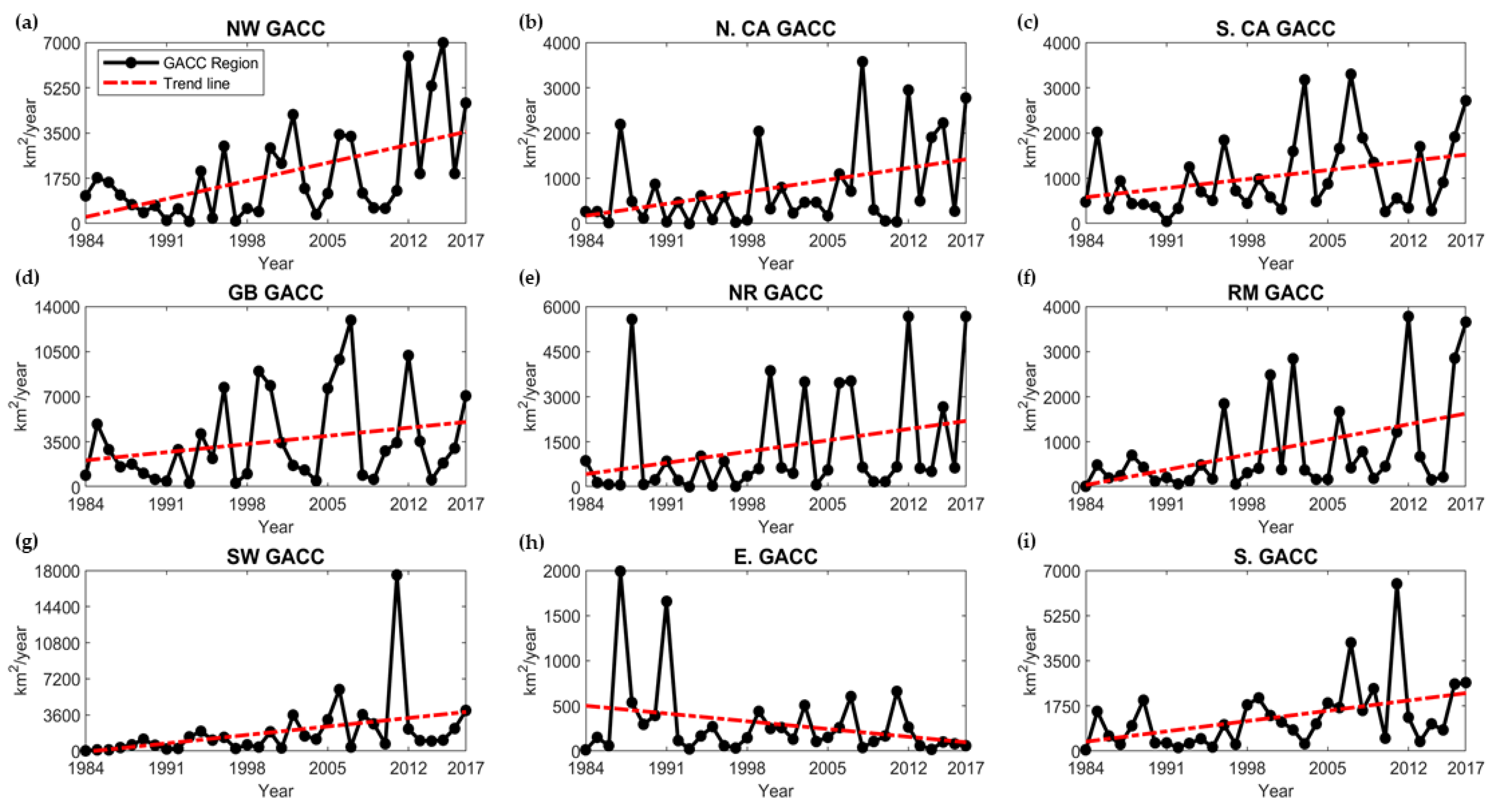
3.1. Total Burned Area Trends of the Nine GACC Regions

The Mann–Kendall test (p < 0.05) determined that out of the nine GACC regions, only five regions show statistically significant trends in the total burned area parameter and all demonstrate increasing trends over time (seen in Figure 3). These regions are the following: NW, NR, RM, SW, and S. The linear regression results depict that the GACC wildfire regime that has the strongest positive trend over time is the SW GACC, the slope is 120.48 km2/year. Interestingly, the SW GACC has an anomaly in its record, occurring in 2011 (seen in Figure 3), which accounts for approximately 27% of the 34-year total burned area record. Other regions displaying noteworthy positive trends over time are the NW, and GB GACCs (seen in Table 2 and Figure 3); Table 2 summarizes the results of the linear regression, coefficient of determination (R2), and Mann–Kendall test for the three parameters within their respective GACC regions. Whereas, both California GACCs do not demonstrate significant positive trends in the total burned area; however, it should be noted that both regions are experiencing greater variability in more recent years. In regard to which region has the “best” linear fit to our linear model is the NW GACC (R2 = 0.30). Whereas, the GB GACC displays a much weaker linear fit (R2 = 0.06). The E and S GACC exemplify opposing trend directions over the 34-year record (Figure 3h,i) and notable differences in their slope (seen in Table 2). The E GACC is the only region with a negative trend (slope = −12.27 km2/year) in the total burned area parameter and has experienced a fairly stable wildfire regime since the 1990s. Whereas, the S GACC is a region experiencing a gradual rise in the amount of total burned area over time (slope = 57.04 km2/year). Essentially all GACC regions, except for the E GACC, displayed positive trends in the total burned area.

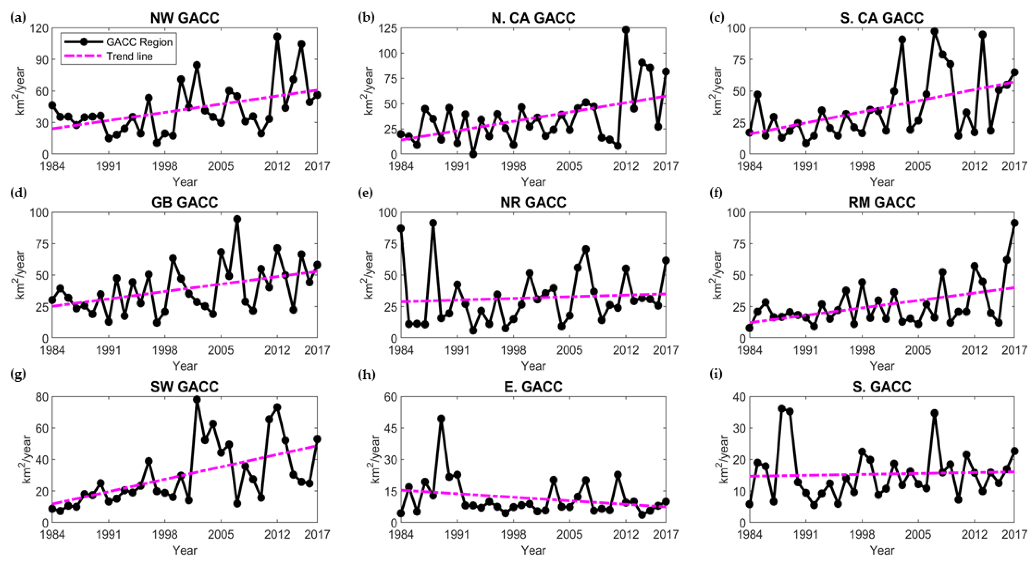
3.2. Frequency Trends of the Nine GACC Regions

The Mann–Kendall test (p < 0.05) determined that out of the nine GACC regions, only five regions display significant frequency trends over time and all demonstrate positive trajectories. These regions are the following GACCs: NW, NR, RM, SW, and S. The linear regression results (seen in Table 2) depict that the GACC wildfire regime that shows the strongest positive trend over time is the S GACC, the slope is 3.13 counts/year. However, the S GACC exemplifies much variability in the occurrence of large wildfires (defined in this region as 500 (2.02 km2) acres or greater) since 1997. The GACCs in the Western US that are experiencing a relatively “strong” positive frequency trend (large wildfires defined as 1000 (4.05 km2) acres or greater) are the NR GACC (slope is 1.27 counts/year) and the SW GACC (slope is 1.87 counts/year). The linear regression results also determined that the S GACC has the best linear fit over time (R2 = 0.28), with the NW GACC closely following it (R2 = 0.24). As seen in Figure 4, the E GACC is no longer the only GACC region defined by a negative trend over time; the SCA GACC is also framed by a negative trend. It is clear that with a declining total burned area trend for the E GACC, there is a corresponding negative frequency trend. However, the SCA GACC shows a positive total burned area trend. These opposing trends suggest that larger wildfires over time are occurring at a less frequent rate in the region. The remaining GACCs (NCA, GB, and NR) all demonstrate gradual positive trends over time. It appears that most of the GACC regions that presented positive trends in the total burned area are also displaying positive trends in the frequency trends, except for the SCA GACC.

3.3. Average Burned Area of the Nine GACC Regions

The results from the third analyzed parameter, average burned area per year, gives another view on how total burned area and frequency are interconnected. This allows for some understanding of how fire size is changing over time within the confines of CONUS. The NCA, SCA, and GB GACCs did not show any statistically significant trends under the Mann–Kendall test for the total burned area and frequency parameters. However, the average burned area parameter for all of the three aforementioned GACCs shows significant positive trends as indicated in Figure 5 and Table 2. In addition to the previously mentioned GACCs, the SW (R2 = 0.32), and NW (R2 = 0.22) GACCs also demonstrate significant trends in regard to the average burned area parameter. The NW and SW GACC regions showed statistically significant trends in every parameter analyzed. It implies that the NW and SW GACCs encompass wildfire regimes that have shown the greatest changes within the period in a positive trajectory. The NR, RM, and S GACCs all have slight gradual positive trends, with the RM GACC having the best linear fit (R2 = 0.21) out of the three. As seen in Figure 5, the E GACC displayed a negative trend and could not be characterized as having a significant trend. Hence, the E GACC is the region which is experiencing a relatively gradual decline in the total burned area, frequency, and average burned area trends. It is also the only GACC region to exemplify no statistically significant trends in any of the three observed parameters. However, these results imply that the E GACC is showing a decrease in frequency and burned area in regard to large wildfires, but does not incorporate the effect of smaller wildfires in the region. The NR and S GACCs are defined by average burned area trends that are relatively flat (seen in Figure 5), which is a characterization that was not seen in the total burned area and frequency parameters. Therefore, the average burned area parameter allows for another view on how to understand the increasing changes of fire regimes which would be limited if the scope of the analysis only incorporated the total burned area and frequency trends.

4. Discussion

Most of the GACC regions exhibit positive trends in the observed wildfire parameters (total burned area, frequency, average burned area). Lightning-caused wildfires were most prominent in the Northwest forested mountains ecoregion [23] which could have played a large role in the significant wildfire trends observed in the NW GACC. The NCA GACC is a fire regime that exemplifies energy-limited characteristics [55]. This is because large fires can occur with temperatures rising to a limit that dries out the plethora of fuel that exists in the region because it is a relatively dense forested ecosystem [55]. In addition, within the Mediterranean California and Marine West Coast Forests ecoregions it was demonstrated that as biomass increased, large fire size increased, a possible by-product of fuel continuity [22]. The aforementioned phenomenon could be a factor that could explain the significant average burned area trend not only seen in the NCA GACC but also the SCA GACC. The SCA GACC demonstrates a moisture-limited regime where large fires can occur because of successful rain events that lead to fuel accumulation [55]. Hence, when this increased fuel load is dried out it can exacerbate the occurrence of large fires [55]. Now, a possible explanation for the decreasing trend in the frequency of the SCA GACC region can be related to the most recent drought years in the region (2011–2015) because it is a region that largely relies on fuel accumulation. It has been projected that the area burned by Southern California wildfires in May-September, which are not driven by the Santa winds, would increase by 77% because of the warmer and drier climate under the representative concentration pathway 8.5 scenario [56]. The GB GACC is a region with increases in fire frequency and area burned in recent years which have been in connection with the invasion of nonnative annual grasses across large portions of the region [21]. The aforementioned factor is a possible explanation in the observed significant average burned area parameter.
The NR and RM GACCs demonstrate an increase in wildfire activity, especially during the last decade. This is a possible response to climate change, and the gradual accumulation of fuel because of the fire management practice of fire suppression within the Rocky Mountain forests [57]. Fire suppression is more relevant to the current increase in fire activity in the NR and RM GACCs because fire suppression efforts lead to increasing fuel loading and continuity on most forested landscapes in the Western US [40]. The SW GACC presents an interesting case regarding the total burned area and frequency parameters. In 2011, the SW GACC experienced the largest total burned area and the greatest count of fire frequency. The observed record-breaking burned area, during 2011, is interesting because drought conditions did exist in the area, but it was not exceptionally warm throughout Arizona and New Mexico, where record-breaking forest fires occurred [58]. Hence, the total burned area in the SW GACC, in 2011, was very likely promoted by record-low precipitation and record-high vapor-pressure deficit (VPD) [58]. More importantly, the SW GACC is a region with significant trends in every observed wildfire parameter. This could be because of increasing temperature, and vapor pressure deficit trends and decreasing precipitation trends since 1984 [37].
On the other hand, the E GACC exemplifies a decreasing trend in every parameter analyzed; however, no statistically significant trends were observed. However, a study has suggested that the very large fires that occur in the Eastern US are largely related to long-term droughts, especially under sub-seasonal drought and fire-weather conditions [17]. It is also noteworthy that the E GACC encompasses a region that is dominated by human-started wildfires, predominantly in the Spring [23]. The E GACC is projected to have a slight increase in the potential for very large wildfires which could prove to be detrimental on private property and air quality in the more densely populated regions of the Eastern US [24]. As for the S GACC, in recent years, it has shown an increase in total burned area and frequency, which was in agreement with predictions on fire season extension of two to three months for the entire Southern US that will have repercussions on fire management in the future [59]. The S GACC is a region that is also dominated by human-ignited wildfires, primarily in the fall and winter in Texas and the Gulf States [23]. In addition, the S GACC has a noteworthy dissociation between hydrologic variables and burned area because it is a region dominated by human-ignited wildfires [10]. Further, the total burned area of large human-caused wildfires was highest in the Southern Florida region [22]. Moreover, the potential for very large wildfires is projected to increase in the Southern Coastal Plain and most of Florida [24]. Thus, the S GACC is an important region to continue monitoring because of the aforementioned projections and is already exhibiting significant total burned area and frequency trends. The wildfire behavior in the S GACC demonstrates the importance of studying wildfire regimes across CONUS to identify all significant wildfire regimes.
The weighing damage caused by current wildfire trends and the estimated potential damage has motivated policymakers, managers, and communities to develop new systems to better mitigate the changing wildfire regimes across CONUS. This study has identified significant GACC wildfire regimes which is of importance because GACCs are used to develop National Significant Wildland Fire Potential Outlook Maps; a service provided by the National Interagency Coordination Center (NICC) which is part of the National Interagency Fire Center (NIFC) [60]. These maps are designed to provide outlooks for the current month, the next month, and a seasonal look that is two months beyond that [60]. These maps reflect the purpose of GACCs, to improve information available to fire management decision makers. Additionally, when a GACC has depleted its resources it can ask for help from NICC in locating additional resources, air tankers, radios, and many other needed tools to fight wildfires [60]. Furthermore, the usage of GACCs are changing. For example, a study used GACCs to quantify relationships between monthly Artic sea-ice extent and annual wildfire activity in the Western US, using GACCs to determine a potential driver of wildfire activity [61]. A better understanding of how GACC wildfire regimes are evolving over time can improve predictive services (i.e., outlook maps, other fire-related products), help protect lives and property, and improve firefighting efficiency.

5. Conclusions

The web of natural and anthropogenic influences on wildfire regimes has increased wildfire activity; hence, altering wildfire regimes across CONUS. Therefore, the importance of our study is to disentangle which wildfire regimes are exhibiting significant wildfire trends under the GACC premise. Using the GACC level of aggregation allows for wildfire information to be readily available for local, state, and national fire management agencies. Furthermore, GACCs can serve as the framework for a more efficient method of logistical coordination and distribution of resources (e.g., people, aircraft, equipment) within each GACC region, and other GACC regions. Our study demonstrates that all GACC regions across CONUS, except the E GACC, demonstrate at least one or more positive trends in the observed wildfire parameters. Additionally, the NW and SW GACC regions demonstrated statistically significant trends in every observed parameter. Interestingly, the NCA, SCA, and GB GACCs show statistically significant trends in the average burned area parameter. The S GACC is a region that is evolving into a wildfire regime that is largely characterized by the Western US wildfire regimes. Further exploration is needed to understand and quantify which regions within the GACCs are attributed to the significant wildfire trends determined in this study. Ultimately, there is heterogeneity in the observed wildfire trends across CONUS which are mainly increasing over time. This will require a paradigm shift in wildfire management practices to better respond to the current wildfire activity and to prepare for the projected increases in wildfire activity across CONUS.

Author Contributions

Conceptualization, J.L., A.F. and J.T.R.; formal analysis, J.S. and A.F.; funding acquisition, J.L.; investigation, J.S.; methodology, J.S., J.L., A.F. and J.T.R.; resources, J.L. and J.T.R.; software, J.S., J.L. and A.F.; supervision, J.L., A.F. and J.T.R.; writing—original draft preparation, J.S.; writing—review and editing, J.L., A.F. and J.T.R. All authors have read and agreed to the published version of the manuscript.

Funding

This research was funded by the NASA Minority University Research and Education Project (MUREP) Institutional Research Opportunity grant, grant number NNX15AQ06A.

Acknowledgments

The authors would like to thank the anonymous reviewers for their helpful comments which we believe improved the clarify of the manuscript. The spatial and tabular data was provided by the Monitoring Trends in Burn Severity Project which is supported by the USGS Earth Resources Observations Systems Data Center and the USDA Forest Service Remote Sensing Applications Center.

Conflicts of Interest

The authors declare no conflict of interest.

References

  1. McWethy, D.B.; Schoennagel, T.; Higuera, P.E.; Krawchuk, M.; Harvey, B.J.; Metcalf, E.C.; Schultz, C.; Miller, C.; Metcalf, A.L.; Buma, B.; et al. Rethinking Resilience to Wildfire. Nat. Sustain. 2019, 2, 797–804. [Google Scholar] [CrossRef]
  2. Moritz, M.A.; Batllori, E.; Bradstock, R.A.; Gill, A.M.; Handmer, J.; Hessburg, P.F.; Leonard, J.; McCaffrey, S.; Odion, D.C.; Schoennagel, T.; et al. Learning to Coexist with Wildfire. Nature 2014, 515, 58–66. [Google Scholar] [CrossRef] [PubMed]
  3. USDA/FS. The Rising Cost of Wildfire Operations: Effect on the Forest Service’s Non-Fire Work. Available online: https://www.fs.usda.gov/sites/default/files/2015-Fire-Budget-Report.pdf (accessed on 27 July 2020).
  4. Bowman, D.M.J.S.; Balch, J.K.; Artaxo, P.; Bond, W.J.; Carlson, J.M.; Cochrane, M.A.; D’Antonio, C.M.; DeFries, R.S.; Doyle, J.C.; Harrison, S.P.; et al. Fire in the Earth System. Science 2009, 324, 481–485. [Google Scholar] [CrossRef] [PubMed]
  5. Finco, M.; Quayle, B.; Zhang, Y.; Lecker, J.; Megown, K.A.; Brewer, K.C. Monitoring Trends and Burn Severity (MTBS): Monitoring Wildfire Activity for the Past Quarter Century Using Landsat Data. In Proceedings of the Forest Inventory and Analysis (FIA) Symposium 2012, Baltimore, MD, USA, 4–6 December 2012; p. 7. [Google Scholar]
  6. Calkin, D.E.; Thompson, M.P.; Finney, M.A.; Hyde, K.D. A Real-Time Risk Assessment Tool Supporting Wildland Fire Decisionmaking. J. For. 2011, 109, 274–280. [Google Scholar]
  7. Abatzoglou, J.T.; Kolden, C.A. Relationships between Climate and Macroscale Area Burned in the Western United States. Int. J. Wildland Fire 2013, 22, 1003. [Google Scholar] [CrossRef]
  8. National Geographic Coordination Centers Website Portal about Us Page. Available online: https://gacc.nifc.gov/admin/about_us/about_us.htm (accessed on 1 June 2020).
  9. Kolden, C.A. We’re Not Doing Enough Prescribed Fire in the Western United States to Mitigate Wildfire Risk. Fire 2019, 2, 30. [Google Scholar] [CrossRef] [Green Version]
  10. Farahmand, A.; Stavros, E.N.; Reager, J.T.; Behrangi, A.; Randerson, J.T.; Quayle, B. Satellite Hydrology Observations as Operational Indicators of Forecasted Fire Danger across the Contiguous United States. Nat. Hazards Earth Syst. Sci. 2020, 20, 1097–1106. [Google Scholar] [CrossRef] [Green Version]
  11. Flannigan, M.D.; Wotton, B.M.; Marshall, G.A.; de Groot, W.J.; Johnston, J.; Jurko, N.; Cantin, A.S. Fuel Moisture Sensitivity to Temperature and Precipitation: Climate Change Implications. Clim. Chang. 2016, 134, 59–71. [Google Scholar] [CrossRef]
  12. Albano, C.M.; Dettinger, M.D.; Soulard, C.E. Influence of Atmospheric Rivers on Vegetation Productivity and Fire Patterns in the Southwestern U.S.: Atmospheric River Effects on. J. Geophys. Res. Biogeosci. 2017, 122, 308–323. [Google Scholar] [CrossRef]
  13. Xiao, J.; Zhuang, Q. Drought Effects on Large Fire Activity in Canadian and Alaskan Forests. Environ. Res. Lett. 2007, 2, 044003. [Google Scholar] [CrossRef]
  14. Shabbar, A.; Skinner, W.; Flannigan, M.D. Prediction of Seasonal Forest Fire Severity in Canada from Large-Scale Climate Patterns. J. Appl. Meteorol. Climatol. 2011, 50, 785–799. [Google Scholar] [CrossRef]
  15. Abatzoglou, J.T.; Kolden, C.A. Climate Change in Western US Deserts: Potential for Increased Wildfire and Invasive Annual Grasses. Rangel. Ecol. Manag. 2011, 64, 471–478. [Google Scholar] [CrossRef]
  16. Archer, S.R.; Predick, K.I. Climate Change and Ecosystems of the Southwestern United States. Rangelands 2008, 30, 23–28. [Google Scholar] [CrossRef] [Green Version]
  17. Barbero, R.; Abatzoglou, J.T.; Kolden, C.A.; Hegewisch, K.C.; Larkin, N.K.; Podschwit, H. Multi-Scalar Influence of Weather and Climate on Very Large-Fires in the Eastern United States: Weather, climate and very large-fires in the eastern united states. Int. J. Clim. 2015, 35, 2180–2186. [Google Scholar] [CrossRef]
  18. Westerling, A.L. Warming and Earlier Spring Increase Western U.S. Forest Wildfire Activity. Science 2006, 313, 940–943. [Google Scholar] [CrossRef] [Green Version]
  19. Littell, J.S.; McKenzie, D.; Peterson, D.L.; Westerling, A.L. Climate and Wildfire Area Burned in Western U.S. Ecoprovinces, 1916–2003. Ecol. Appl. 2009, 19, 1003–1021. [Google Scholar] [CrossRef]
  20. Jensen, D.; Reager, J.T.; Zajic, B.; Rousseau, N.; Rodell, M.; Hinkley, E. The Sensitivity of US Wildfire Occurrence to Pre-Season Soil Moisture Conditions across Ecosystems. Environ. Res. Lett. 2018, 13, 014021. [Google Scholar] [CrossRef]
  21. Dennison, P.E.; Brewer, S.C.; Arnold, J.D.; Moritz, M.A. Large Wildfire Trends in the Western United States, 1984-2011: Large wildfire trends in the western us. Geophys. Res. Lett. 2014, 41, 2928–2933. [Google Scholar] [CrossRef]
  22. Nagy, R.C.; Fusco, E.; Bradley, B.; Abatzoglou, J.T.; Jennifer, B. Human-Related Ignitions Increase the Number of Large Wildfires across U.S. Ecoregions. Fire 2018, 1, 4. [Google Scholar] [CrossRef] [Green Version]
  23. Balch, J.K.; Bradley, B.A.; Abatzoglou, J.T.; Nagy, R.C.; Fusco, E.J.; Mahood, A.L. Human-Started Wildfires Expand the Fire Niche across the United States. Proc. Natl. Acad. Sci. USA 2017, 114, 2946–2951. [Google Scholar] [CrossRef] [Green Version]
  24. Barbero, R.; Abatzoglou, J.T.; Larkin, N.K.; Kolden, C.A.; Stocks, B. Climate Change Presents Increased Potential for Very Large Fires in the Contiguous United States. Int. J. Wildl. Fire 2015, 24, 892. [Google Scholar] [CrossRef]
  25. Abatzoglou, J.T.; Williams, A.P. Impact of Anthropogenic Climate Change on Wildfire across Western US Forests. Proc. Natl. Acad. Sci. USA 2016, 113, 11770–11775. [Google Scholar] [CrossRef] [Green Version]
  26. Cattau, M.E.; Wessman, C.; Mahood, A.; Balch, J.K. Anthropogenic and Lightning-started Fires Are Becoming Larger and More Frequent over a Longer Season Length in the U.S.A. Glob. Ecol. Biogeogr. 2020, 29, 668–681. [Google Scholar] [CrossRef]
  27. Radeloff, V.C.; Helmers, D.P.; Kramer, H.A.; Mockrin, M.H.; Alexandre, P.M.; Bar-Massada, A.; Butsic, V.; Hawbaker, T.J.; Martinuzzi, S.; Syphard, A.D.; et al. Rapid Growth of the US Wildland-Urban Interface Raises Wildfire Risk. Proc. Natl. Acad. Sci. USA 2018, 115, 3314–3319. [Google Scholar] [CrossRef] [Green Version]
  28. Short, K.C. A spatial database of wildfires in the United States, 1992–2011. Earth Syst. Sci. Data 2014, 1–27. [Google Scholar] [CrossRef] [Green Version]
  29. Malone, S.L.; Kobziar, L.N.; Staudhammer, C.L.; Abd-Elrahman, A. Modeling Relationships among 217 Fires Using Remote Sensing of Burn Severity in Southern Pine Forests. Remote Sens. 2011, 3, 2005–2028. [Google Scholar] [CrossRef] [Green Version]
  30. Szpakowski, D.M.; Jensen, J.L.R. A Review of the Applications of Remote Sensing in Fire Ecology. Remote Sens. 2019, 11, 2638. [Google Scholar] [CrossRef] [Green Version]
  31. Sankey, J.B.; Wallace, C.S.A.; Ravi, S. Phenology-Based, Remote Sensing of Post-Burn Disturbance Windows in Rangelands. Ecol. Indic. 2013, 30, 35–44. [Google Scholar] [CrossRef]
  32. Coen, J.L.; Schroeder, W. Use of Spatially Refined Satellite Remote Sensing Fire Detection Data to Initialize and Evaluate Coupled Weather-Wildfire Growth Model Simulations: Wildfire modeling using fire detection. Geophys. Res. Lett. 2013, 40, 5536–5541. [Google Scholar] [CrossRef]
  33. Eidenshink, J.; Schwind, B.; Brewer, K.; Zhu, Z.-L.; Quayle, B.; Howard, S. A Project for Monitoring Trends in Burn Severity. Fire Ecol. 2007, 3, 3–21. [Google Scholar] [CrossRef]
  34. Lutz, J.A.; Key, C.H.; Kolden, C.A.; Kane, J.T.; van Wagtendonk, J.W. Fire Frequency, Area Burned, and Severity: A Quantitative Approach to Defining a Normal Fire Year. Fire Ecol. 2011, 7, 51–65. [Google Scholar] [CrossRef]
  35. Barbero, R.; Abatzoglou, J.T.; Steel, E.A.; Larkin, N.K. Modeling Very Large-Fire Occurrences over the Continental United States from Weather and Climate Forcing. Environ. Res. Lett. 2014, 9, 124009. [Google Scholar] [CrossRef]
  36. Holden, Z.A.; Swanson, A.; Luce, C.H.; Jolly, W.M.; Maneta, M.; Oyler, J.W.; Warren, D.A.; Parsons, R.; Affleck, D. Decreasing Fire Season Precipitation Increased Recent Western US Forest Wildfire Activity. Proc. Natl. Acad. Sci. USA 2018, 115, E8349–E8357. [Google Scholar] [CrossRef] [PubMed] [Green Version]
  37. Mueller, S.E.; Thode, A.E.; Margolis, E.Q.; Yocom, L.L.; Young, J.D.; Iniguez, J.M. Climate Relationships with Increasing Wildfire in the Southwestern US from 1984 to 2015. For. Ecol. Manag. 2020, 460, 117861. [Google Scholar] [CrossRef]
  38. Williams, A.P.; Abatzoglou, J.T.; Gershunov, A.; Guzman-Morales, J.; Bishop, D.A.; Balch, J.K.; Lettenmaier, D.P. Observed Impacts of Anthropogenic Climate Change on Wildfire in California. Earth’s Future 2019, 7, 892–910. [Google Scholar] [CrossRef] [Green Version]
  39. Donovan, V.M.; Wonkka, C.L.; Twidwell, D. Surging Wildfire Activity in a Grassland Biome: Surging Wildfire Activity in a Grassland. Geophys. Res. Lett. 2017, 44, 5986–5993. [Google Scholar] [CrossRef]
  40. Calkin, D.E.; Thompson, M.P.; Finney, M.A. Negative Consequences of Positive Feedbacks in US Wildfire Management. For. Ecosyst. 2015, 2, 9. [Google Scholar] [CrossRef] [Green Version]
  41. Cochrane, M.A.; Moran, C.J.; Wimberly, M.C.; Baer, A.D.; Finney, M.A.; Beckendorf, K.L.; Eidenshink, J.; Zhu, Z. Estimation of Wildfire Size and Risk Changes Due to Fuels Treatments. Int. J. Wildl. Fire 2012, 21, 357. [Google Scholar] [CrossRef] [Green Version]
  42. Joseph, M.B.; Rossi, M.W.; Mietkiewicz, N.P.; Mahood, A.L.; Cattau, M.E.; St. Denis, L.A.; Nagy, R.C.; Iglesias, V.; Abatzoglou, J.T.; Balch, J.K. Spatiotemporal Prediction of Wildfire Size Extremes with Bayesian Finite Sample Maxima. Ecol. Appl. 2019, 29. [Google Scholar] [CrossRef] [Green Version]
  43. Kolden, C.A.; Smith, A.M.S.; Abatzoglou, J.T. Limitations and Utilisation of Monitoring Trends in Burn Severity Products for Assessing Wildfire Severity in the USA. Int. J. Wildl. Fire 2015, 24, 1023. [Google Scholar] [CrossRef]
  44. Parker, B.M.; Lewis, T.; Srivastava, S.K. Estimation and Evaluation of Multi-Decadal Fire Severity Patterns Using Landsat Sensors. Remote Sens. Environ. 2015, 170, 340–349. [Google Scholar] [CrossRef]
  45. Monitoring Trends in Burn Severity Website Frequently Asked Questions Page. Available online: https://www.mtbs.gov/faqs (accessed on 27 July 2020).
  46. United States Geological Survey Website Landsat Missions Page. Available online: https://www.usgs.gov/land-resources/nli/landsat/landsat-satellite-missions?qt-science_support_page_related_con=2#qt-science_support_page_related_con (accessed on 27 July 2020).
  47. Parks, S.; Dillon, G.; Miller, C. A New Metric for Quantifying Burn Severity: The Relativized Burn Ratio. Remote Sens. 2014, 6, 1827–1844. [Google Scholar] [CrossRef] [Green Version]
  48. Syphard, A.D.; Radeloff, V.C.; Keeley, J.E.; Hawbaker, T.J.; Clayton, M.K.; Stewart, S.I.; Hammer, R.B. Human influence on california fire regimes. Ecol. Appl. 2007, 17, 1388–1402. [Google Scholar] [CrossRef] [PubMed]
  49. Westerling, A.L. Increasing Western US Forest Wildfire Activity: Sensitivity to Changes in the Timing of Spring. Phil. Trans. R. Soc. B 2016, 371, 20150178. [Google Scholar] [CrossRef]
  50. Su, X.; Yan, X.; Tsai, C.-L. Linear Regression: Linear Regression. WIREs Comp. Stat. 2012, 4, 275–294. [Google Scholar] [CrossRef]
  51. Mann, H.B. Nonparametric Tests Against Trend. Econometrica 1945, 13, 245. [Google Scholar] [CrossRef]
  52. Kendall, M.G. Rank Correlation Methods, 4th ed.; Charles Griffin: London, UK, 1975; Available online: https://psycnet.apa.org/record/1948-15040-000 (accessed on 27 July 2020).
  53. Hamed, K.H.; Rao, A.R. A Modified Mann-Kendall Trend Test for Autocorrelated Data. J. Hydrol. 1998, 204, 182–196. [Google Scholar] [CrossRef]
  54. Yue, S.; Pilon, P.; Cavadias, G. Power of the Mann–Kendall and Spearman’s Rho Tests for Detecting Monotonic Trends in Hydrological Series. J. Hydrol. 2002, 259, 254–271. [Google Scholar] [CrossRef]
  55. Westerling, A.L.; Bryant, B.P. Climate Change and Wildfire in California. Clim. Chang. 2008, 87, 231–249. [Google Scholar] [CrossRef]
  56. Jin, Y.; Goulden, M.L.; Faivre, N.; Veraverbeke, S.; Sun, F.; Hall, A.; Hand, M.S.; Hook, S.; Randerson, J.T. Identification of Two Distinct Fire Regimes in Southern California: Implications for Economic Impact and Future Change. Environ. Res. Lett. 2015, 10, 094005. [Google Scholar] [CrossRef] [Green Version]
  57. Schoennagel, T.; Veblen, T.T.; Romme, W.H. The Interaction of Fire, Fuels, and Climate across Rocky Mountain Forests. Biol. Sci. 2004, 54, 661. [Google Scholar] [CrossRef]
  58. Williams, A.P.; Seager, R.; Berkelhammer, M.; Macalady, A.K.; Crimmins, M.A.; Swetnam, T.W.; Trugman, A.T.; Buenning, N.; Hryniw, N.; McDowell, N.G.; et al. Causes and Implications of Extreme Atmospheric Moisture Demand during the Record-Breaking 2011 Wildfire Season in the Southwestern United States. J. Appl. Meteorol. Climatol. 2014, 53, 2671–2684. [Google Scholar] [CrossRef]
  59. Mitchell, R.J.; Liu, Y.; O’Brien, J.J.; Elliott, K.J.; Starr, G.; Miniat, C.F.; Hiers, J.K. Future Climate and Fire Interactions in the Southeastern Region of the United States. For. Ecol. Manag. 2014, 327, 316–326. [Google Scholar] [CrossRef]
  60. National Interagency Coordination Center Website National Significant Wildland Fire Potential Outlook Page. Available online: https://www.nifc.gov/nicc/predictive/outlooks/outlooks.htm (accessed on 27 July 2020).
  61. Knapp, P.; Soulé, P. Spatio-Temporal Linkages between Declining Arctic Sea-Ice Extent and Increasing Wildfire Activity in the Western United States. Forests 2017, 8, 313. [Google Scholar] [CrossRef] [Green Version]
Figure 1. MTBS data (1984–2017), represented in the figure as black incident points, is overlaid across Contiguous US (CONUS) and framed by the nine Geographic Area Coordination Center (GACC) regions. The label for each GACC is seen in the legend.
Remotesensing 12 02565 g001
Figure 2. The general process of this study to obtain wildfire time series over CONUS from 1984 to 2017. Each wildfire time series is fitted with a linear trend using linear regression methods and tested for significance under the Mann–Kendall test.
Remotesensing 12 02565 g002
Figure 3. (ai) Time series of the nine GACC regions (1984–2017) for the parameter of total burned area per year. Each time series is fitted with a trend line, in red, using linear regression techniques (least-squares method).
Remotesensing 12 02565 g003
Figure 4. (ai) Time series of the nine GACC regions (1984–2017) for the parameter of frequency per year. Each time series is fitted with a trend line, in blue, using linear regression techniques (least-squares method).
Remotesensing 12 02565 g004
Figure 5. (ai) Time series of the nine GACC regions (1984–2017) for the parameter of average burned area per year. Each time series is fitted with a trend line, in purple, using linear regression techniques (least-squares method).
Remotesensing 12 02565 g005
Table 1. Landsat missions incorporated for the development of the Monitoring Trends in Burn Severity (MTBS) database.
Satellite Mission 1Sensor TypeElectromagnetic Spectrum Region 2Wavelength Range (μm)Band Position
Landsat 4
(1982–1993)
Thematic Mapper NIR0.76–0.904
SWIR2.08–2.357
Landsat 5
(1984–2013)
Thematic MapperNIR0.76–0.904
SWIR2.08–2.357
Landsat 7
(1999–Present)
Enhanced Thematic Mapper +NIR0.77–0.904
SWIR2.08–2.357
Landsat 8
(2013–Present)
Operational Land ImagerNIR0.85–0.885
SWIR22.11–2.297
1 The time period listed is the corresponding mission time frame; not the satellite usage by the MTBS database. 2 NIR = Near-Infrared, SWIR = Shortwave Infrared, SWIR2 = Shortwave Infrared region used by the MTBS database that exists in Landsat 8.
Table 2. Characterization of the nine GACC regions based on the metrics of the three parameters analyzed.
GACC RegionParameterSlope 1R2Trend DirectionSignificance 2 (p < 0.05)
Total Burned Area99.850.30 *
NorthwestFrequency0.990.24 *
Avg. Burned Area1.110.22 *
Total Burned Area37.780.15
N. CaliforniaFrequency0.290.03
Avg. Burned Area1.320.24 *
Total Burned Area28.500.11
S. CaliforniaFrequency−0.160.02
Avg. Burned Area1.250.24 *
Total Burned Area90.170.07
Great BasinFrequency0.460.009
Avg. Burned Area0.840.19 *
Total Burned Area53.590.09 *
N. RockiesFrequency1.270.19 *
Avg. Burned Area0.190.008
Total Burned Area480.20 *
Rocky MtnFrequency0.680.1 *
Avg. Burned Area0.840.21
Total Burned Area120.480.15 *
SouthwestFrequency1.870.14 *
Avg. Burned Area1.120.32 *
Total Burned Area−12.270.08
EasternFrequency−0.480.05
Avg. Burned Area−0.240.07
Total Burned Area57.040.19 *
SouthernFrequency3.130.28 *
Avg. Burned Area0.040.003
1 The unit of the slope for both Total Burned Area and Average Burned Area parameters is km2/year, while the unit of the slope for the Frequency parameter is counts/year. 2 Trend significance at a 95% confidence interval was conducted using the Mann–Kendall test. The significant trend is marked with an asterisk (*) for the parameter.

