Combining Interior Orientation Variables to Predict the Accuracy of Rpas–Sfm 3D Models

Abstract

Remotely piloted aerial systems (RPAS) have been recognized as an effective low-cost tool to acquire photogrammetric data of low accessible areas reducing collection and processing time. Data processing techniques like structure from motion (SfM) and multiview stereo (MVS) techniques, can nowadays provide detailed 3D models with an accuracy comparable to the one generated by other conventional approaches. Accuracy of RPAS-based measures is strongly dependent on the type of adopted sensors. Nevertheless, up to now, no investigation was done about relationships between camera calibration parameters and final accuracy of measures. In this work, authors tried to fill this gap by exploring those dependencies with the aim of proposing a prediction function able to quantify the potential final error in respect of camera parameters. Predictive functions were estimated by combining multivariate and linear statistical techniques. Four photogrammetric RPAS acquisitions were considered, supported by ground surveys, to calibrate the predictive model while a further acquisition was used to test and validate it. Results are preliminary, but promising. The calibrated predictive functions relating camera internal orientation (I.O.) parameters with final accuracy of measures (root mean squared error) showed high reliability and accuracy.

1. Introduction

Descriptions of the earth’s morphology and environmental processes involve the adoption of a large amount of data from a wide range of branches of knowledge, such as geology [1], hydrology [2] and geomorphology [3]. All of them require a digital surface model (DSM) as the basis to describe surface morphometry. DSM resolution and accuracy strongly affect landforms mapping: in fact, geomorphic elements, located at the same position, can be differently interpreted depending on DSM resolution [4]. Consequently, DSM resolution must be consistent with the size of the investigated element to optimize results [5]. Along the years, several approaches were proposed to improve 3D models accuracy and detail level of survey. Among these, terrestrial laser scanner (TLS) was widely considered as the gold standard to meet such requirements [6], even if its application determines high costs of both technological equipment and acquisition/processing data time. Researchers looked for a valid low-cost alternative to overcome these operational limits. Rieke-Zapp et al. [7] demonstrated that photogrammetry is a convincing tool to generate 3D models having comparable accuracy and resolution in respect of those from TLS.

RPAS (remotely piloted aerial systems) represent the most significant innovation affecting the photogrammetric field: they allow flights over low accessible areas, are timely flexible and permit detailed acquisitions at low minimizing cloud cover related issues [8]. Moreover, they deeply penetrated the market stimulating the development of new sensors and determining a significant reduction of related costs [9]. Recent technological advances have permitted weight and size reduction of sensors making them suitable for small flying platforms [9]. Data processing techniques have also improved: in particular, structure from motion (SfM) and computer vision (CV) approaches enormously empowered the photogrammetric workflow in terms of accuracy, spatial resolution and easiness. Consequently, the integration of RPAS, SfM and CV nowadays allows to generate highly detailed textured models comparable to those generated through more traditional methods.

For these reasons, RPAS have been widely proposed to face various environmental issues [10,11,12,13,14]. Many scholars have focused on factors influencing the final accuracy of RPAS measurements. Flight height and sensor technical features (pixel size, focal length, sensor size, etc.) together with sensor interior orientation modeling can strongly affect final results [15,16]. A validated methodology for maximizing reliability of the final products was designed by [17,18], taking into account several aspects like: (a) influence of flight plan geometry [11,19]; (b) impact of ground control points (GCPs) georeferencing and distribution [20,21,22]; (c) optimization of parameterization during the bundle adjustment phase [23,24].

In this context, a key element is the estimation of camera calibration coefficients. In fact, RPAS are commonly equipped with low-cost, nonmetric cameras whose internal orientation (I.O.) is natively unknown and must be, somehow, estimated [25]. Focal length (f), principal point offset (x_p, y_p), radial (K₁, K₂, K₃, K₄) and decentering (P₁, P₂, P₃, P₄) coefficients of lens distortion functions are the main I.O. parameters. Their knowledge is essential to generating accurate measurements, but, while using SfM, they show a strong geometric instability depending on the low photogrammetric quality of the camera [26]. Differently, for CV-based applications focal length is the only parameter considered in the camera calibration procedure [27]. Moreover, as demonstrated in [28], the I.O. parameter estimation from a low-cost, nonmetric camera are extremely complex and, sometimes, impossible. To face this issue, numerous algorithms have been implemented in the most widespread photogrammetric software, e.g., Agisoft PhotoScan Professional (Agisoft LLC—St. Petersburg, Russia) [29], Pix4D [30], APERO [31], Graphos [32], VisualSFM [33] and MicMac [34]. Nevertheless, results do not seem to be stable and vary according to the processed set of images, even if referred to the same area [35]. Much research has explored the impact of camera calibration parameters on the final results, but without trying to model the existing relationship [36].

This study is intended to fill this gap by exploring the relationship among I.O. parameter estimates and modeling predictive functions. These goals were achieved with reference to several sets of data collected in different times on the same area: the shoreline of Torre a Mare (Bari, Southern Italy), well known for the beauty of its landscape. Finally, a new approach, based on combination of uni- and multivariate statistics, suitable for predicting error components affecting final 3D models is proposed.

2. Materials and Methods

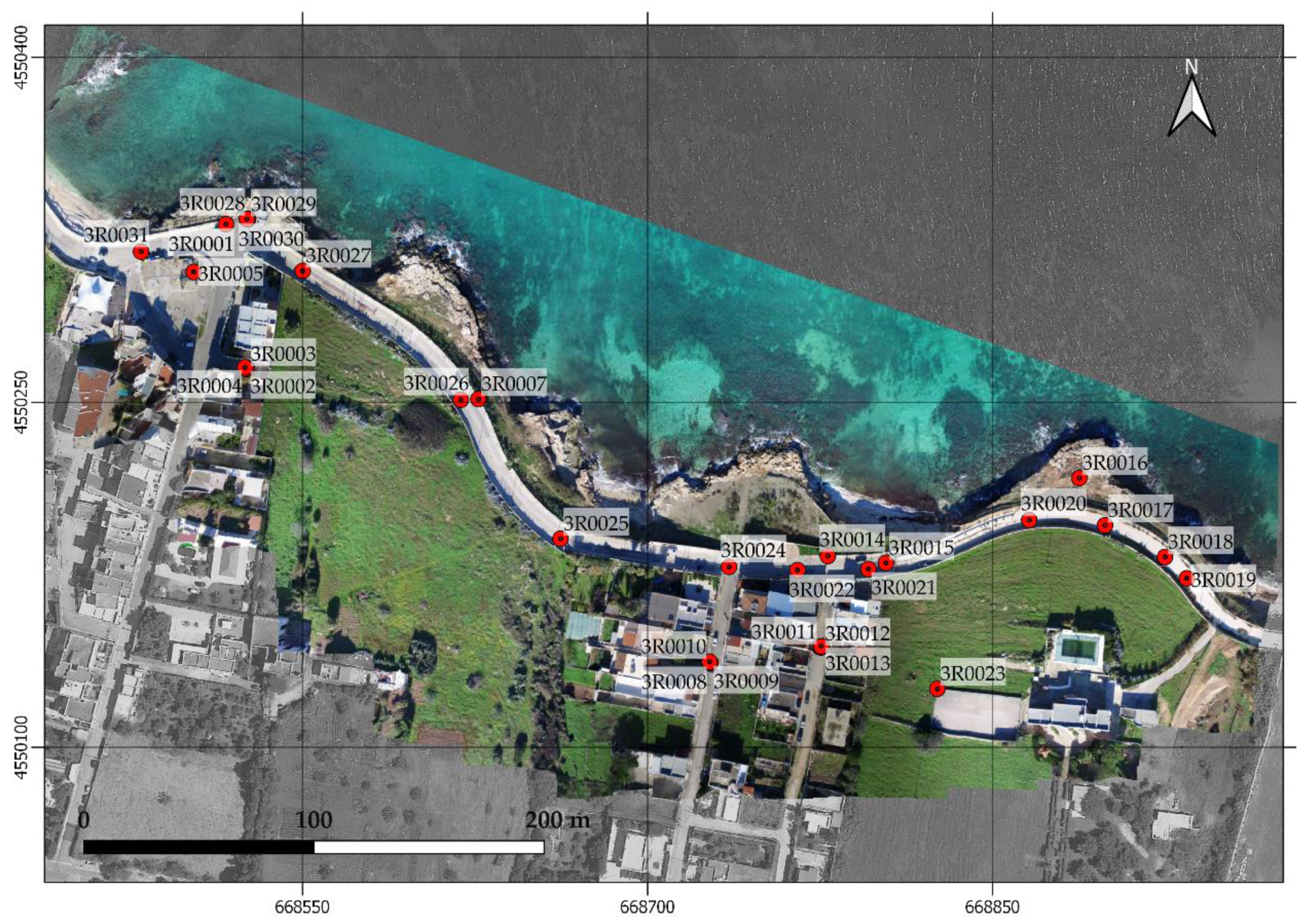
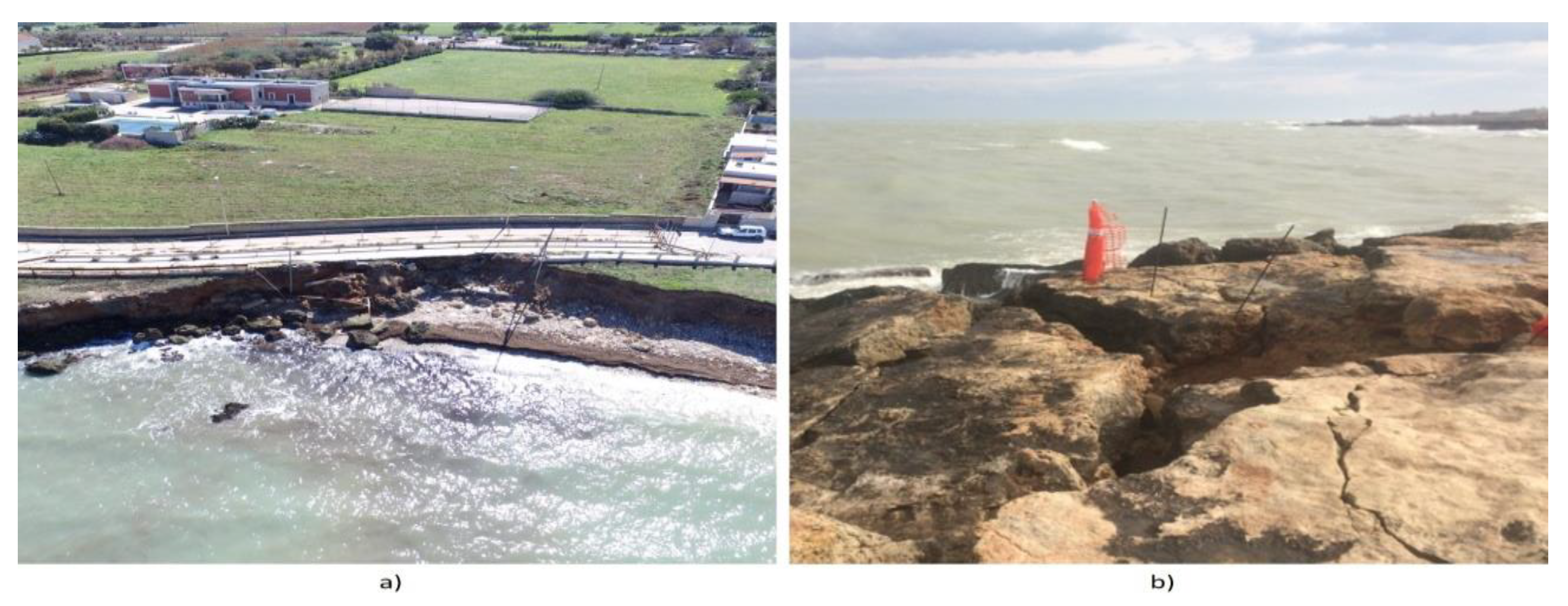
2.1. Study Area

A shoreline stretch of about 400 m located in Torre a Mare (Apulian region), a district 12 km away from Bari, was selected as pilot site. The area presents a rugged coastline, characterized by an irregular elevation ranging between 1 and 5 m—with a large number of small sandy bays and coves (Figure 1) [20]. Over the years, reefs collapsed, and their shapes were modeled by anthropic and natural phenomena, including soil erosion by sea tides, determining a typical stepped profile. Slopes are pointed, while overlying surfaces, dated back to the Upper Pleistocene age, are more shaped and smoothed. Geologists confirmed the wide morphogenetic variability of coastline structure in this area [20].

Subhorizontal surfaces, close to the reef, are mainly composed of calcarenitic lithotypes showing a peculiar resistance to mechanical erosion processes. At the global scale, stratified layers and fracturing systems, subparallel to the coastline (ONO ESE), determine favorable conditions for land instability due to hydric erosion, accelerating natural withdrawal of coast fractions (Figure 2). Moreover, local lack of vegetation increases imperviousness and, consequently, facilitate erosion dynamics [32]. The area is extremely complex from the archaeological perspective, as well. It hosts archeological evidence of a Neolithic community that was pulled out by excavation campaigns carried out in the past; currently, the area is in an evident state of abandon ([37,38]).

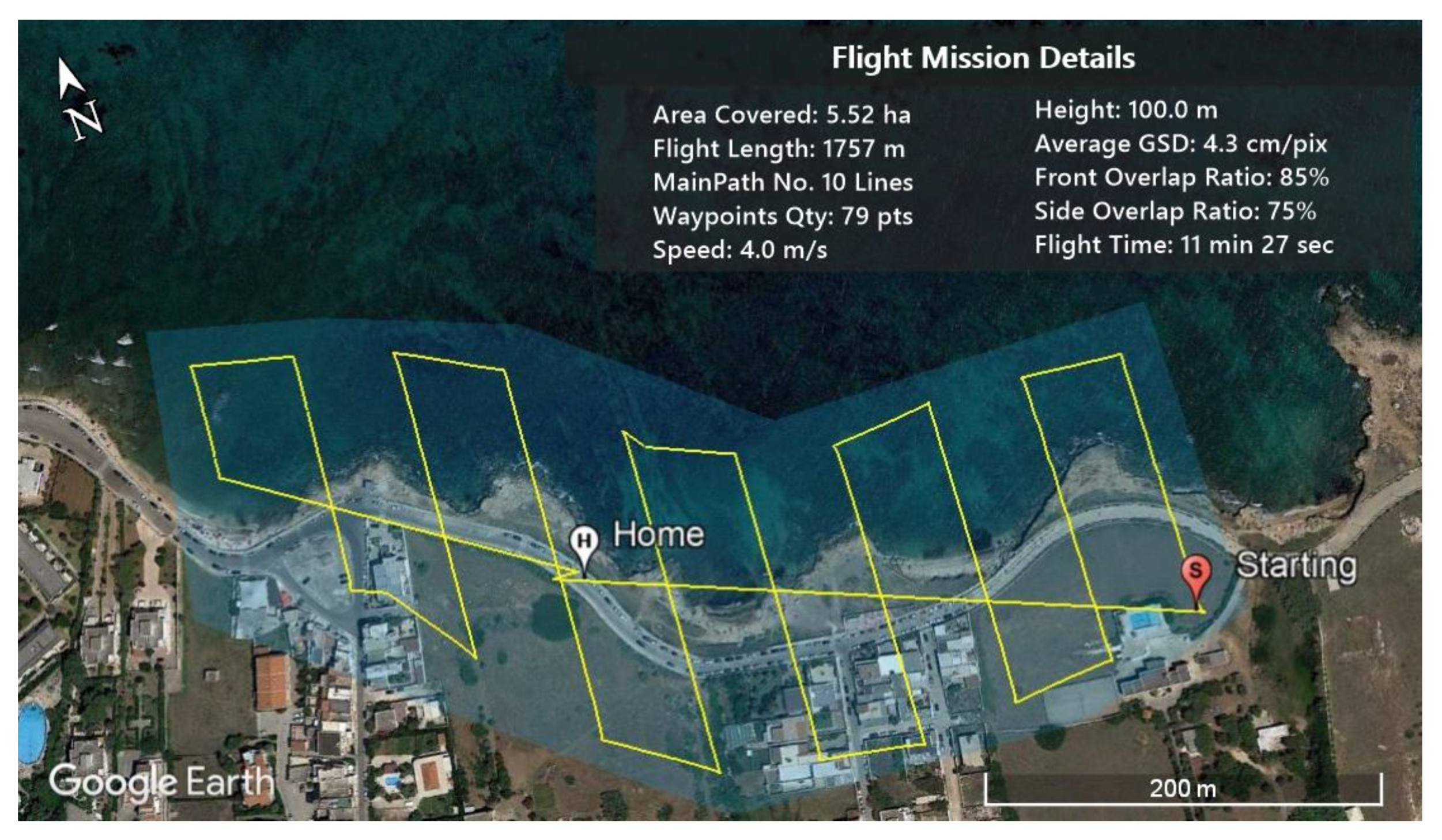
2.2. Field Data Campaigns and Operative Workflow

An extensive flight campaign was planned between 2018 and 2019. Flight area was selected far away from urban sites, to compliant Italian national regulations about RPAS operations [39,40]. Five flights were programmed and performed in December 2018, January 2019, February 2019, March 2019 and October 2019, respectively (

Table 1. Photogrammetric datasets acquired during the five remotely piloted aerial systems (RPAS) campaigns and related ground sample distance (GSD) values.

Acquisition Date	#N Images	GSD (M/Pix)
December 12, 2018	77	0.041
January 8, 2019	77	0.047
February 19, 2019	77	0.048
March 16, 2019	77	0.041
October 16, 2019	77	0.042

). Surveys were interrupted between April and September 2019 to respect operational restrictions related to touristic season [39].

Flight were operated by a commercial quadcopter DJI Inspire 1, mounting a consumer DJI Zenmuse X3 camera (focal length 3.61 mm, pixel size 1.56 μm, effective pixels 12.4 M) equipped with a 3−axis gimbal (to compensate accidental movements of the drone). The DJI Ground Station Pro app, proposed by the Chinese company DJI (Dà−Jiāng Innovations) [41] was also used to automatize the flight plan. It ensured that all the flights were achieved along the same path and under the same conditions, e.g., cruising speed (4.0 m/s) and altitude (100 m AGL, above ground level) (Figure 3). Missions were planned to obtain an average Ground Sampling Distance (GSD) of 0.043 m/pix, a forward and side overlaps of 85% and 75%, respectively, as suggested by [42,43]. A total of 77 images per flight were acquired. Camera was set nadiral and the stop&go mode was applied to reduce collection of blurry images due to forward motion [42]. RPAS position was recorded by a low cost GNSS/INS positioning receiver and saved into a metadata file.

To operate all along the tests with the same ground control points, a GNSS survey campaign was operated to position permanent natural elements having adequate size and color with respect to RPAS image features. Thirty homogeneously distributed points were consequently, surveyed by Leica Viva CS10/GS10 GNSS receiver and successively used as ground control points (GCP) or check points (CPs). Survey was operated in a network real time kinematic (NRTK) mode based on Leica SmartNet Italpos network and determined a final 3D accuracy of 0.02 m. Reference system was RDN2008/UTM zone 33N (NE) (EPSG: 6708).

Image datasets were separately processed according to the workflow of Figure 4. Image blocks of December, January, February and October, were used to calibrate the predictive model (see forward on), while the March dataset was used for validation.

2.3. Photogrammetric Products Generation

This study relies on the workflow proposed by [11,44,45,46]. The work flowchart is shown in Figure 5; steps are detailed in the next sections. Agisoft PhotoScan (v.1.4.1, Agisoft LLC −St. Petersburg, Russia) software, currently known as Metashape, was used during the work to photogrammetrically process the data.

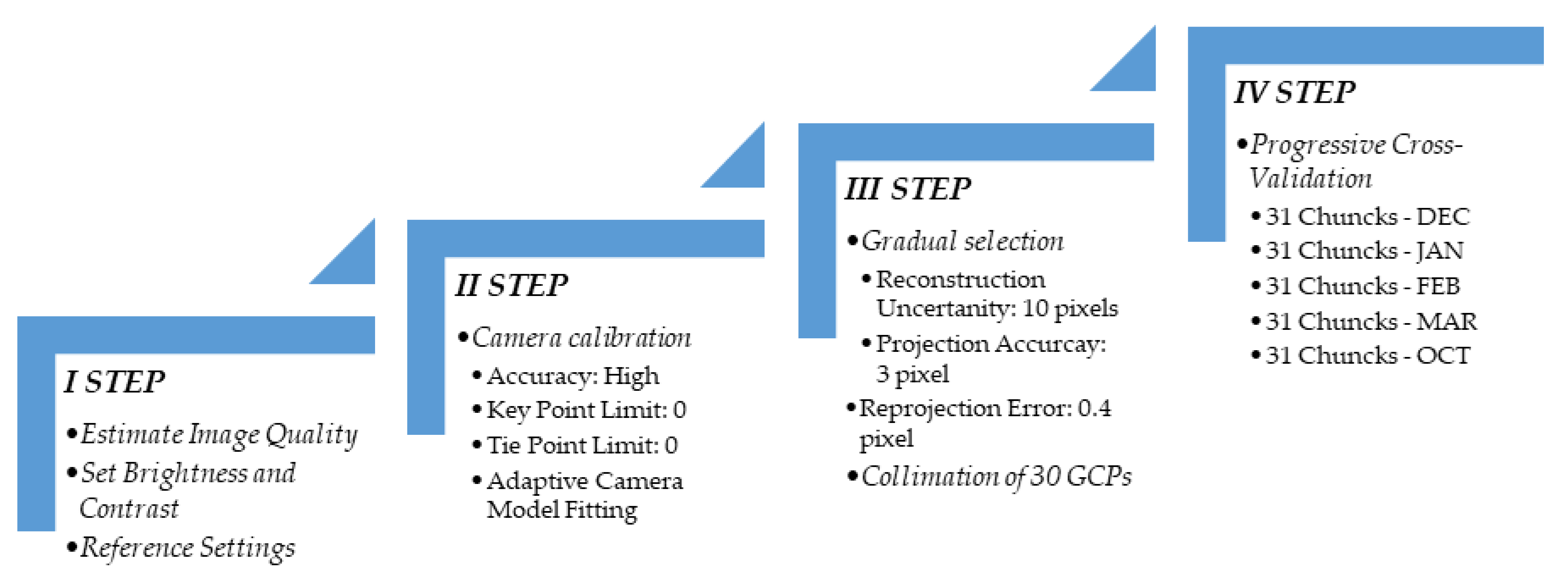
2.3.1. First Step: Setting-Up Workspace and Dataset

This first step was aimed at properly setting workspace and removing blurry images, possibly compromising final outcomes. Five chunks (image blocks) of the same scenario were created and, for each of them, the same processing parameters were set to guarantee results comparability (

Table 2. Agisoft PhotoScan software parameters used during processing of photogrammetric datasets.

Agisoft PhotoScan Parameter	Value
Coordinate system	RDN2008/UTM Zone 33N (NE) (EPSG: 6708)
Initial principal point position (Xp, Yp)	(0, 0)
Camera positioning accuracy	3 m
Camera accuracy, attitude	10 deg
3D marker accuracy (object space)	0.02 m
Marker accuracy (image space)	0.5 pixel
GPS/INS offset vector value	$\Delta x=0.005\pm 0.002\mathrm{m}$ $\Delta y=0.100\pm 0.01\mathrm{m}$ $\Delta z=0.250\pm 0.01\mathrm{m}$

).

Camera positioning accuracy was set equal to 3 m to make it consistent with the average 3D positioning accuracy value of the RPAS GNSS receiver (approximately 2.54 m). This value is known to depend on GNSS epoch recording frequency (Hz) and, consequently, on RPAS speed [46]. Image attitude accuracy was set equal to the software default value (10 degrees) since no information was available about attitude measurements from RPAS-integrated IMU (inertial measurement unit). This value was considered precautionary. Agisoft PhotoScan allows weights parameters during bundle block adjustment (BBA): tie points estimation are generally three times less relevant than GCPs accuracy during the reconstruction phase [17]. Thus, a value equal to 3 was set in its parameterization. All of these parameters are crucial being directly involved in collinearity equations [47,48,49] and, consequently, they heavily affect final accuracy of solution. Software default values were instead accepted as weights for attitude parameters (yaw, tilt, roll).

A quality assessment was performed to detect and remove “bad” images. This step is mandatory to improve final accuracy. A large number of issues conditioning image quality depends on the acquisition mode. For instance, the adoption of RPAS to image a complex scenario, like the study area, involves several problems due to the interaction between environmental conditions and equipment; in particular, heat and magnetic sources can impact on inertial measurement unit (IMU) and GNSS [8]. The “estimate image quality” procedure available within Agisoft PhotoScan was used to assess image characteristics, providing information about sharpness and detecting blurring and distortion. This procedure returns a score ranging between 0 and 1: the higher the value, the better the quality [50,51]. Moreover, to balance colors of final products, all images were homogenized in terms of brightness and contrast. Radiometric adjustments are known to do not condition the efficiency of SIFT algorithm during tie point detection.

A scale-invariant feature transform (SIFT) approach was used to minimize projection errors [52,53] and facilitate extraction of homologous points independently from brightness conditions, that, in the datasets, were strongly influenced by the presence of sea.

2.3.2. Second Step: Image Block Orientation

The II step was aimed at automatically collecting tie points (sparse points cloud) and solving image orientation [54,55]. It was separately run for each chunk using the ‘High’ accuracy mode and setting a threshold = 0 for the “limits of key points and tie points” parameter. This choice was preferred to avoid uncontrolled filtering of measured points.

Block Bundle Adjustment (BBA) was performed including I.O. parameters within the model unknowns to be estimated using the camera optimization panel available in Agisoft PhotoScan. BBA outputs correspond to the estimates of tie-points coordinates in the object space, I.O. and external orientation (E.O.) parameters, GNSS lever arm offset. Moreover, BBA scales the entire photogrammetric block proportionally with respect to GCPs. Camera I.O. parameters estimates from all the chunks were recorded and organized into a table to be successively analyzed.

2.3.3. Third Step: Filtering and Georeferencing

Sparse point clouds (tie-point positions in the object space) were generated and systematic errors, mainly caused by nonlinear distortions of lens [54], estimated; measured points were manually filtered to optimize results and minimize image block distortions. Three criteria implemented in the “gradual selection” tool were considered: (a) photogrammetric restitution uncertainty; (b) projection accuracy; (c) reprojection error.

(a) is intended to remove points with low base–height ratios [49], i.e., all those points located at the edges of images, generally characterized by a higher degree of restitution uncertainty, that majorly depends on a too small overlapping among pictures. Although this option does not affect final accuracy, it is useful for thinning clouds [56]. Conversely, (b) is aimed at detecting and cleaning out less reliable tie points [49]. A threshold value equal to 3 was used to exclude tie points with an uncertainty 3 times higher than the minimum one; (c) was intended to remove all points with a large residual value in order to decrease drastically restitution errors improving orientation parameters estimates [49]. It is worth to remind that, residuals directly impact on representativeness of the root mean square error (RMSE, [40]) of GCPs and CPs, possibly making it not suitable to define the actual final accuracy of measurements [51].

The three above-mentioned criteria permitted to remove the most of inaccurate points from clouds, thus improving consistency between model and reality. Threshold values adopted for each criterion were defined accordingly to previous works [42,43]. After filtering, about 20% of originally measured points were removed. To further improve geometric modeling of the area, 30 GCPs were used [5], ensuring a marker reprojection error less than 0.5 pixels. Once the alignment step was accomplished, a “progressive” cross-validation analysis was achieved to test actual accuracy of final measurements, as explained in Section 2.3.4.

2.3.4. Fourth Step: Progressive Cross-Validation

With respect to the 30 surveyed points, a cross-validation was run in a progressive mode, i.e., progressively migrating 1 point a time from the training (GCPs) to the validation (CPs) set. The choice of those points to be progressively moved from GCPs to CPs was accomplished in a balanced way; peripheral and central points were alternatively migrated taking care of maintaining a proper spatial distribution of remaining GCPs ([22,57]). Thirty one chunks of CPs were finally obtained varying from 0 (all surveyed points were used as GCPs) to 30 points (all surveyed points were used as CPs and the image orientation completely relied on a direct georeferencing approach) [50,58]. We refer to the 0 CPs situation as complete indirect georeferencing (CIG) and to the 30 CPs situation as direct georeferencing (DG) [21,50]. To make the procedure repeatable, points were imported in the same order for all analyzed subdatasets.

Table 3. List of markers chosen and added as control points (CPs) in each implementation.

#GCP	Label	#GCP	Label
29 GCPs	3R0024	14 GCPS	3R0019
28 GCPs	3R0026	13 GCPS	3R0031
27 GCPs	3R0030	12 GCPS	3R0017
26 GCPs	3R0018	11 GCPS	3R0027
25 GCPs	3R0004	10 GCPS	3R0025
24 GCPs	3R0013	9 GCPS	3R0022
23 GCPs	3R0010	8 GCPS	3R0014
22 GCPs	3R0005	7 GCPS	3R0007
21 GCPs	3R0020	6 GCPS	3R0023
20 GCPs	3R0021	5 GCPS	3R0015
19 GCPs	3R0029	4 GCPS	3R0003
18 GCPs	3R0011	3 GCPS	3R0012
17 GCPs	3R0001	2 GCPS	3R0016
16 GCPs	3R0008	1 GCP	3R0028
15 GCPs	3R0002	0 GCP	3R0009

summarizes the order that was followed while migrating a point from GCP to CP.

Measures accuracy was estimated with reference to RMSE computed for both GCPs and CPs. RMSE was used to quantify error components (definitions are given forward on), with the hypothesis that both random and systematic errors were Gaussian distributed [59]. It is worth to remind that RMSE of GCPs only provide information about the goodness of fitting of calibrated equations, with no concern about the model capability of generalization.

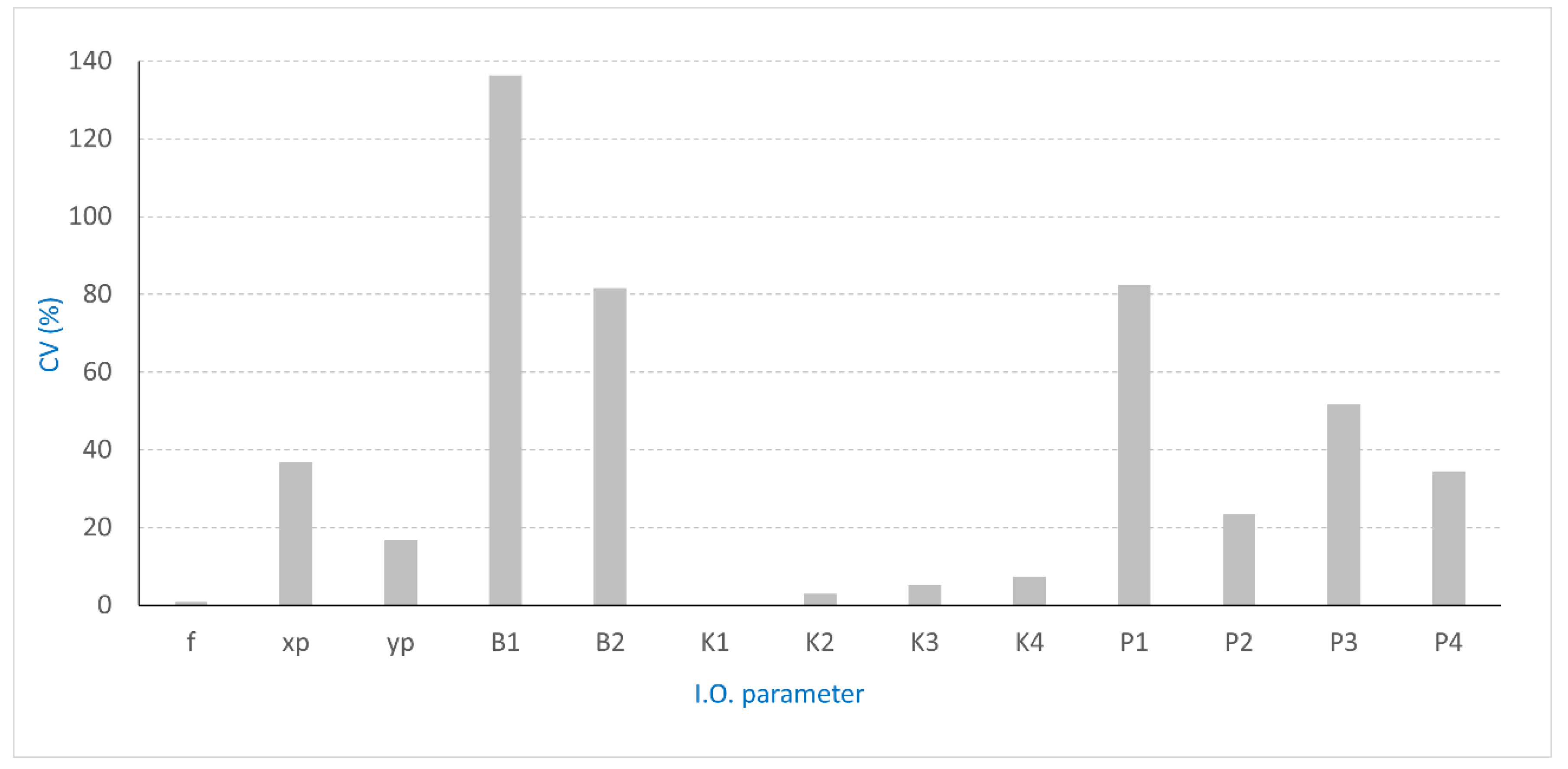
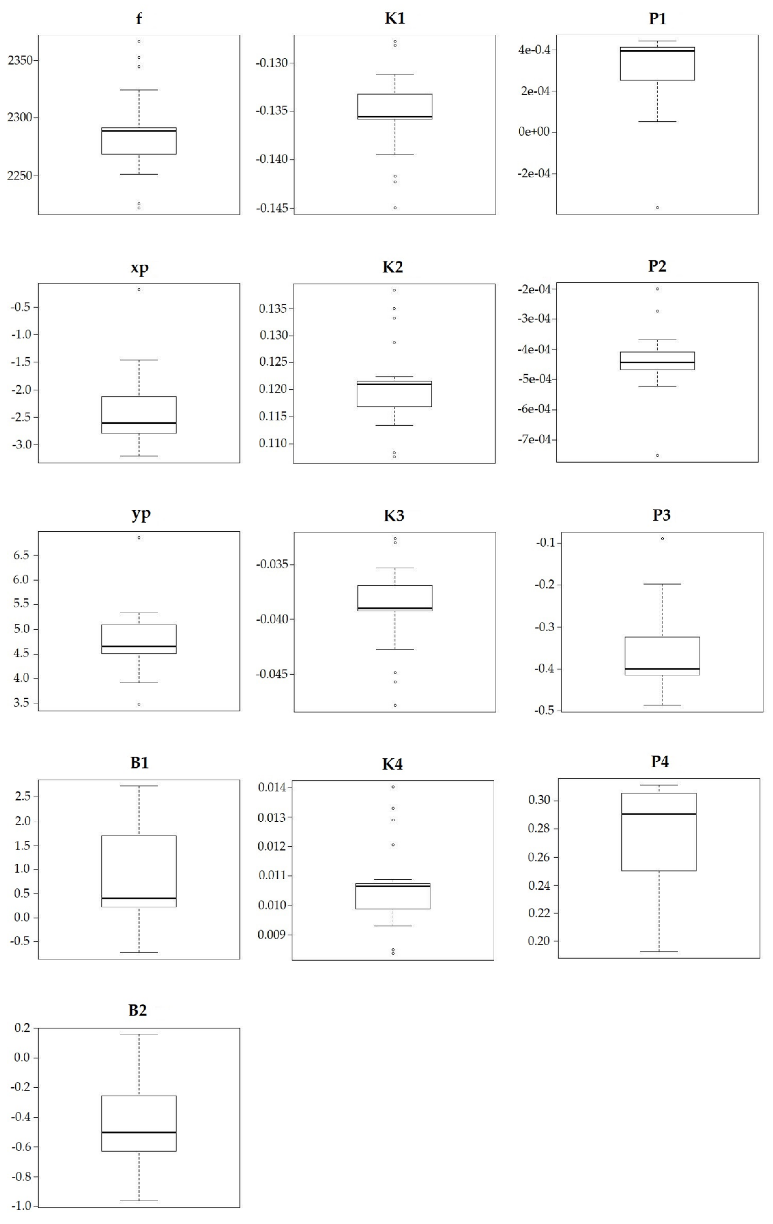
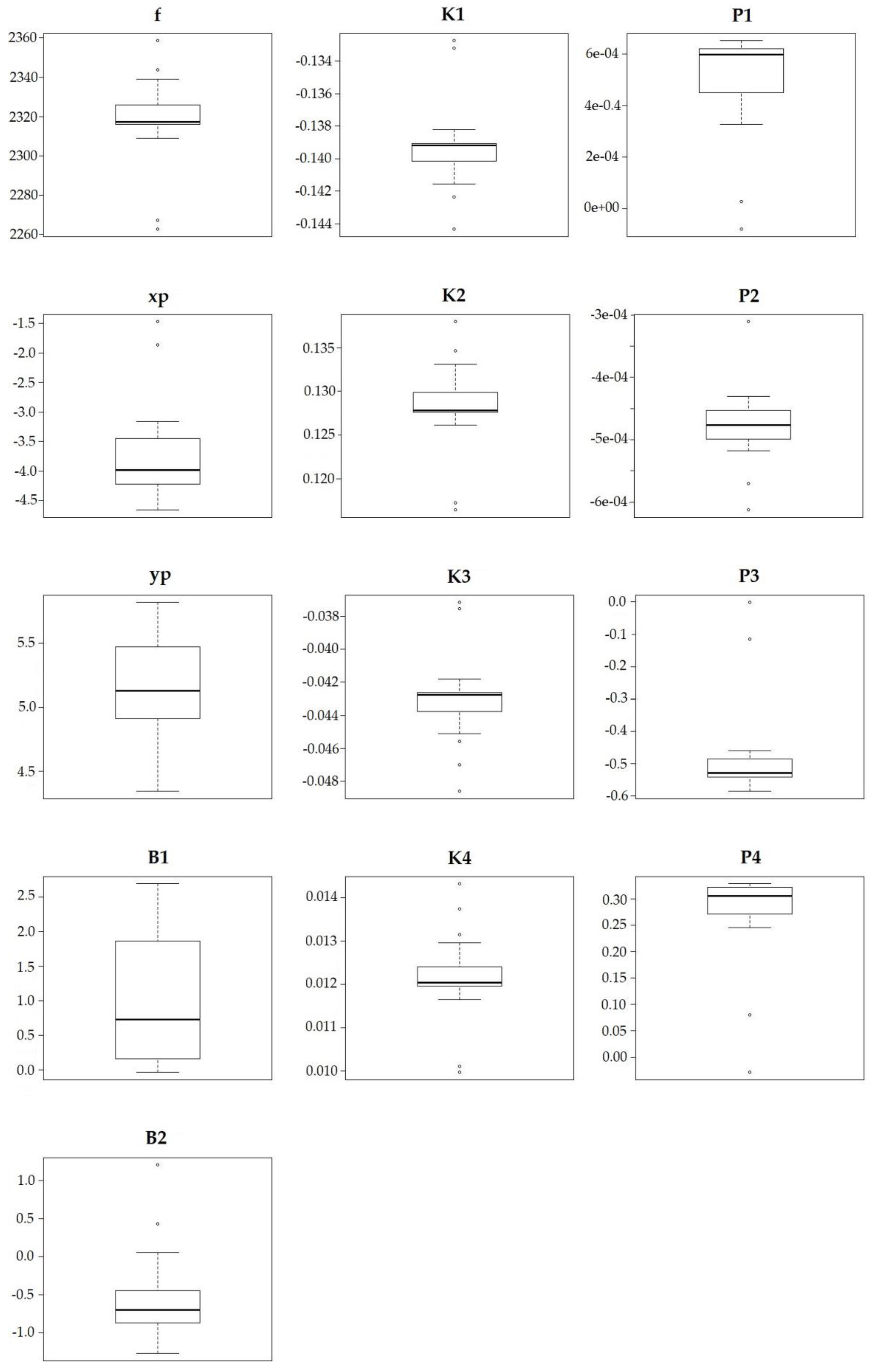
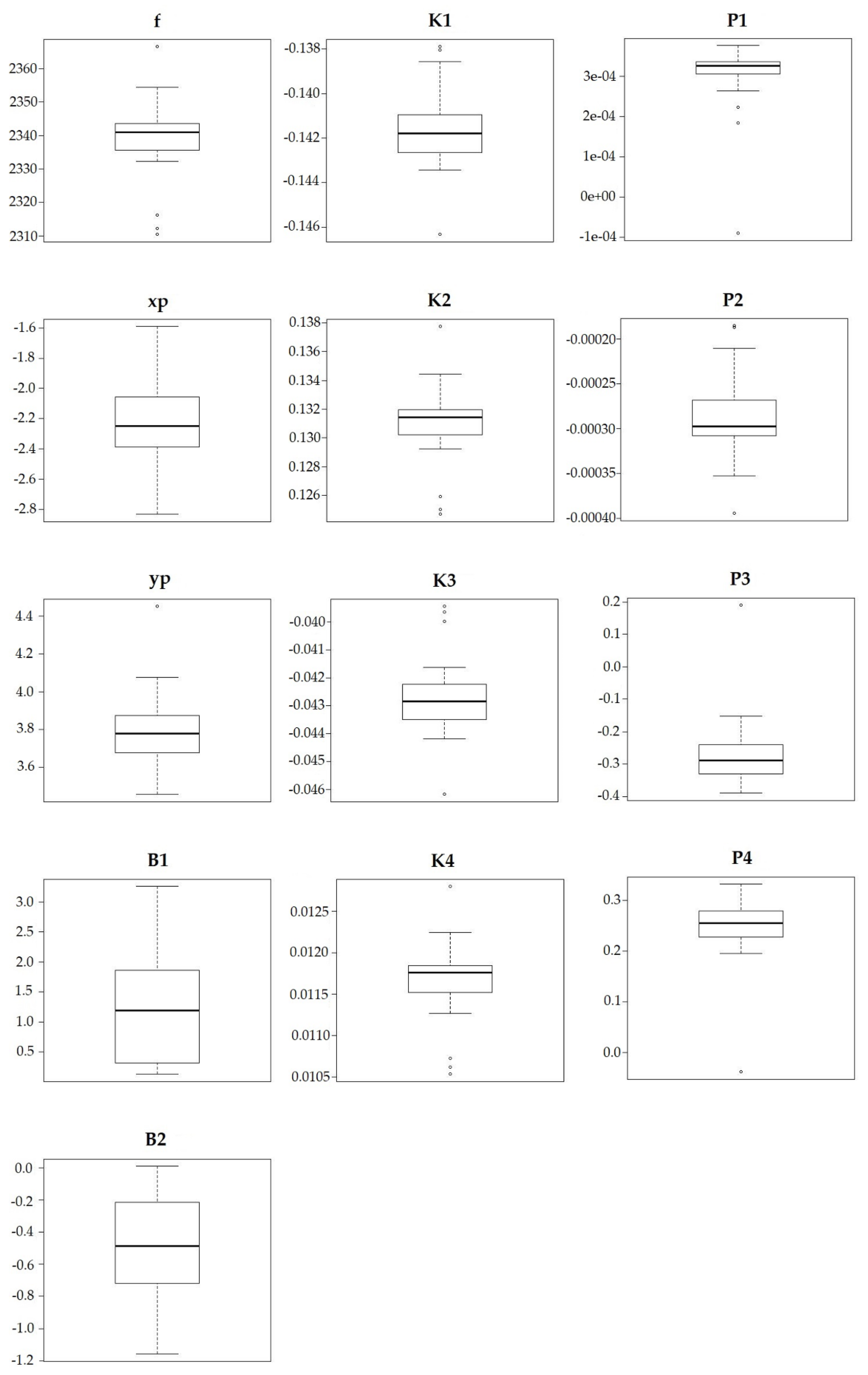
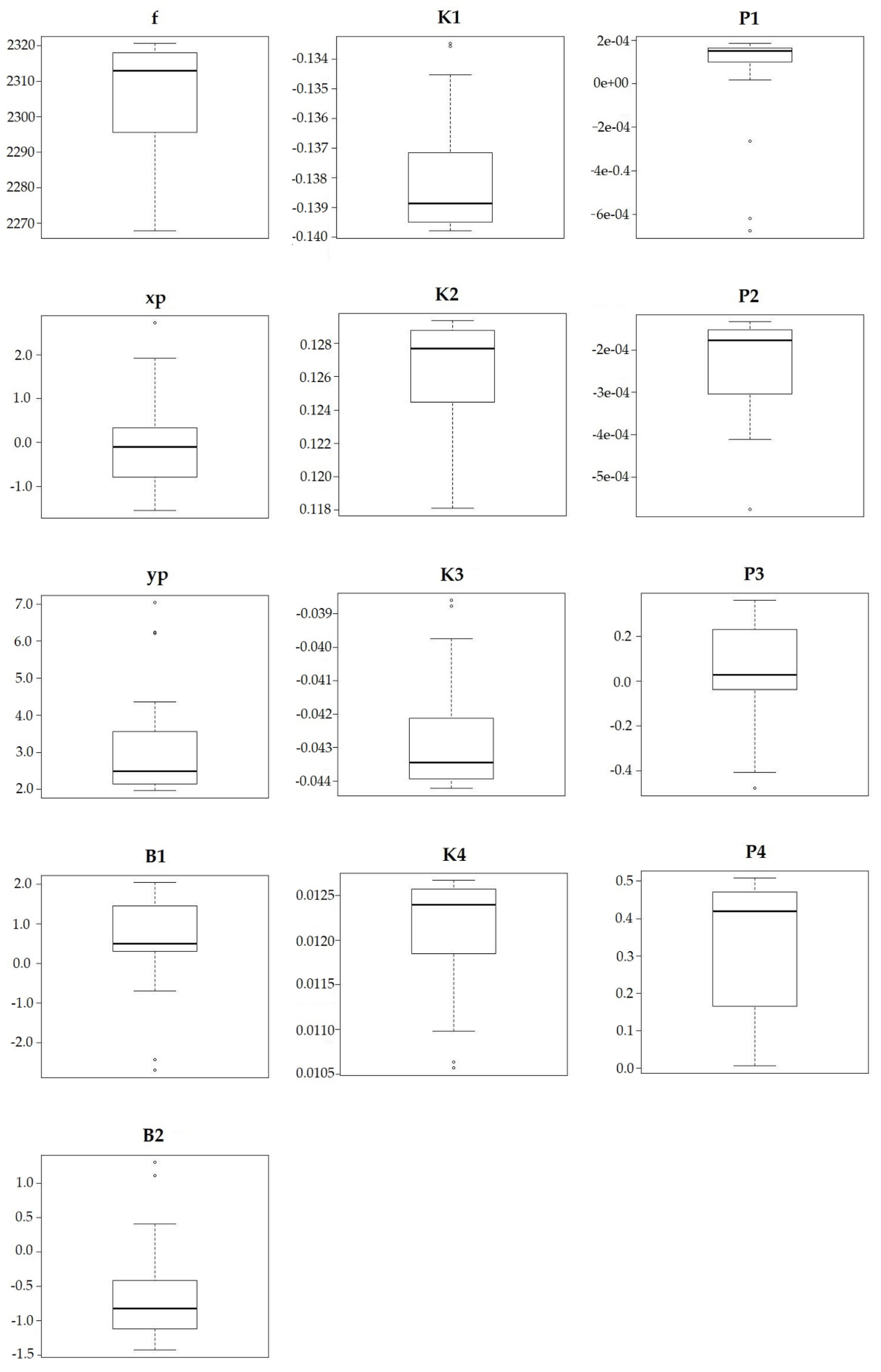
2.4. Analyses of I.O. Parameters Estimates

Camera calibration by SfM implies that camera I.O. parameters (including lens distortion) are precisely known to minimize errors possibly affecting restitution step [60]. Such parameters are image independent and, consequently, they do not depend on position and attitude of the camera [54]. Several approaches have been proposed over the years to get appropriate estimates/measures of these parameters; camera self-calibration guarantees several benefits when working with low-cost cameras. It relies on the numeric estimate of I.O. parameters that are included among the unknowns in the equation system that is solved during BBA. The solution is consistent with the data [61], with the assumption that I.O. parameters continuously vary in time and, consequently, need to be estimated for each specific image block.

Many algorithms can be used when facing this problem by SfM. Agisoft PhotoScan makes available the 10 parameters in Brown’s model [60,62,63,64,65] (Equations (1) and (2), [49].

$$\Delta \mathrm{x}=-\frac{\overline{x}}{c}\Delta f+\overline{x}{r}^2{K}_1+\overline{x}{r}^4{K}_2+\overline{x}{r}^6{K}_3+\overline{x}{r}^8{K}_4+\left[\left(2{\overline{x}}^2+r^2\right)P_1+2P_2\overline{xy}\right]\left(1+P_3{r}^2+P_4{r}^4\right)+B_1\overline{x}+B_2\overline{y}$$

(1)

$$\Delta \mathrm{y}=-\frac{\overline{y}}{c}\Delta f+\overline{y}{r}^2{K}_1+\overline{y}{r}^4{K}_2+\overline{y}{r}^6{K}_3+\overline{x}{r}^8{K}_4+\left[2P_1\overline{xy}+\left(2{\overline{y}}^2+r^2\right)P_2\right]\left(1+P_3{r}^2+P_4{r}^4\right)$$

(2)

where f is the focal length, $\Delta x$ and $\Delta y$ represents the image corrections, $\Delta f$ is the correction to the initial principal distance value, $\overline{x}$ and $\overline{y}$ are the coordinates of a general poin, K_i are the radial distortion coefficients, P_i are the tangential distortion coefficients, B_i are the in-plane correction parameters for differential scaling between the horizontal and vertical pixel spacing and non-orthogonality (axial skew) between x and y axes, r is the image radial distance estimated using Equation (3):

$$r^2={\overline{x}}^2+{\overline{y}}^2={(x-x_p)}^2+{(y-y_p)}^2$$

(3)

where x_p and y_p represents the principal point coordinates.

The full 10-parameter model, Equations (1)–(3), is adopted as the default one when using the fully automatic camera calibration procedure. Although, practically, it could appear as the best choice, from an accuracy point of view, in many cases, it does not represent the optimal solution, because of the different role and significance of those parameters within the BBA numeric solution [55]. For example, a high correlation was found between P_i coefficients and principal point coordinates. Consequently, when removing P_i from the unknowns, x_p and y_p somehow can absorb associated variation. In other words, users could not consider P_i in the calibration phase and obtain similar results. With these premises, a preventive analysis was achieved to figure out eventual correlation existing among I.O. parameters and trying to minimize it.

2.5. Accuracy Assessment

Accuracy assessment was aimed at: (a) testing the quality of the original dataset; (b) testing the accuracy of the photogrammetric measurements.

Triggs et al. [54] highlighted that accuracy of photogrammetric products depends on many factors: quality of the processed images, GSD and camera type. Consequently, all these factors were considered. The first factor was taken into account (trying to minimize its effects) using the image quality tool and selecting a scale-invariant feature transform (SIFT) approach while running BBA by SfM (see Section 2.3.1).

Errors affecting final measures from oriented image blocks were evaluated with reference to the RMSE. It was computed separately for all the error components and for both GCPs and CPs. RMSE_E for the East coordinate, RMSE_N for the North coordinate, RMSE_H for the height coordinate, RMSE_T as the total 3D error and, finally, RMSE_I for the positioning error (total) in the image space.

Agisoft PhotoScan Professional software can automatically and iteratively compute this parameter [48]. This software feature is important, permitting reiteration of trials that can be run selectively tuning all the involved parameters, including GCPs collection refinement.

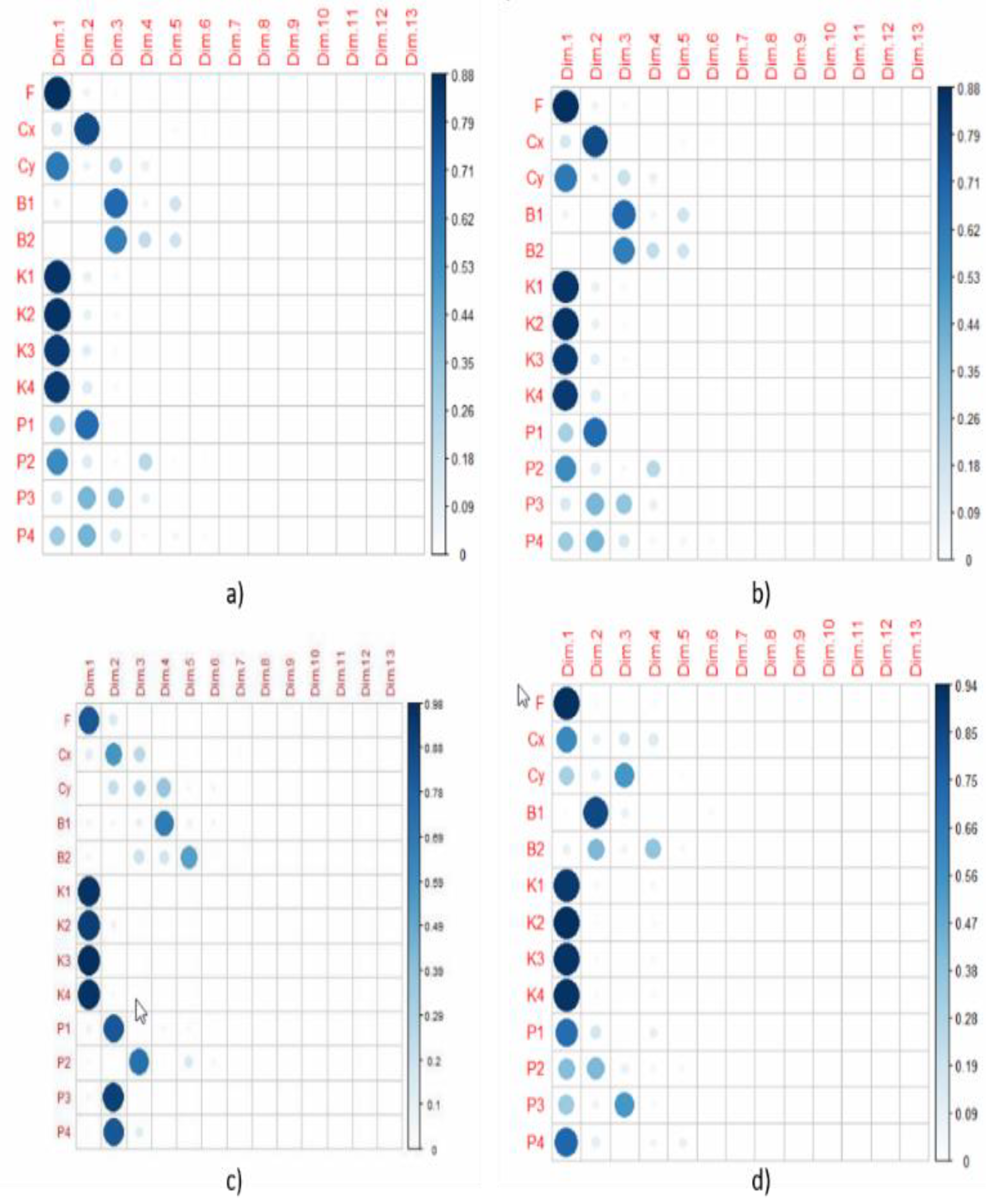
2.6. PCA and Synthetic Index Generation

I.O. estimates and errors computed during BBA were compared to test their reciprocal relationship. I.O. estimates were preventively preprocessed by a self-developed R routine [66] aimed at extracting the most significant information by principal component analysis (PCA), based on the variance maximization principle [67]. PCA, probably the most popular multivariate statistical method, is intended for dimensionality reduction, obtained by removing redundant information of a multivariate dataset where variables can be intercorrelated [67]. After detecting the most relevant components, it converts the original dataset into a new one consisting of independent and orthogonal vectors, called principal components (PCs, [67]). The first component provides the most of information, describing the largest part of the input data inertia, absorbing (explaining) the most of data variance; the second component is orthogonal to the first one and absorbs (explain) the most of the remaining variance [68]. The same principle is used to obtain all the other components that, necessarily, will represent a decreasing level of information while incrementing their position within the transformation [69]. Consequently, first components compress most of the native information making possible to drastically reduce dimensionality of data by removing redundant content [62].

The singular value decomposition (SVD) approach [69] was applied to compute principal components. The number of explanatory PCs was selected by the Kaiser’s criterion [70] that suggest setting an eigenvalue threshold = 1.0. Selected PCs were weighted and linearly combined in a “synthetic index” (hereinafter called SI). SI was obtained as the weighted average of all significant components (Equation (4)). Weights were directly extracted from the PCA procedure:

$$SI=\frac{\sum w_i\ast Di{m}_i}{\sum w_i}$$

(4)

where w_i and Dim_i are the weights and the principal components, respectively.

2.7. Predicting Accuracy of Measurements: Model Definition

Pearson’s coefficient (R) was computed between SI and error components affecting final measurements from oriented blocks. The expectation was that SI could be a predictor of error components (generically called RMSE_j). According to the obtained R values (only high or moderate correlation was considered) an interpolation function was calibrated to predict the following errors: RMSE_E, RMSE_N, RMSE_H, RMSE_T, RMSE_I. SI was assumed as independent variable (x, predictor) of calibrated functions. A 2nd order polynomial (Equation (5)) was found to well fit all significant relationships. Model parameters (a, b and c) were estimated by ordinary least squares for each investigated error (y). Goodness of fitting was tested with reference to the coefficient of determination (R²):

$$y=a{x}^2+bx+c$$

(5)

3. Results

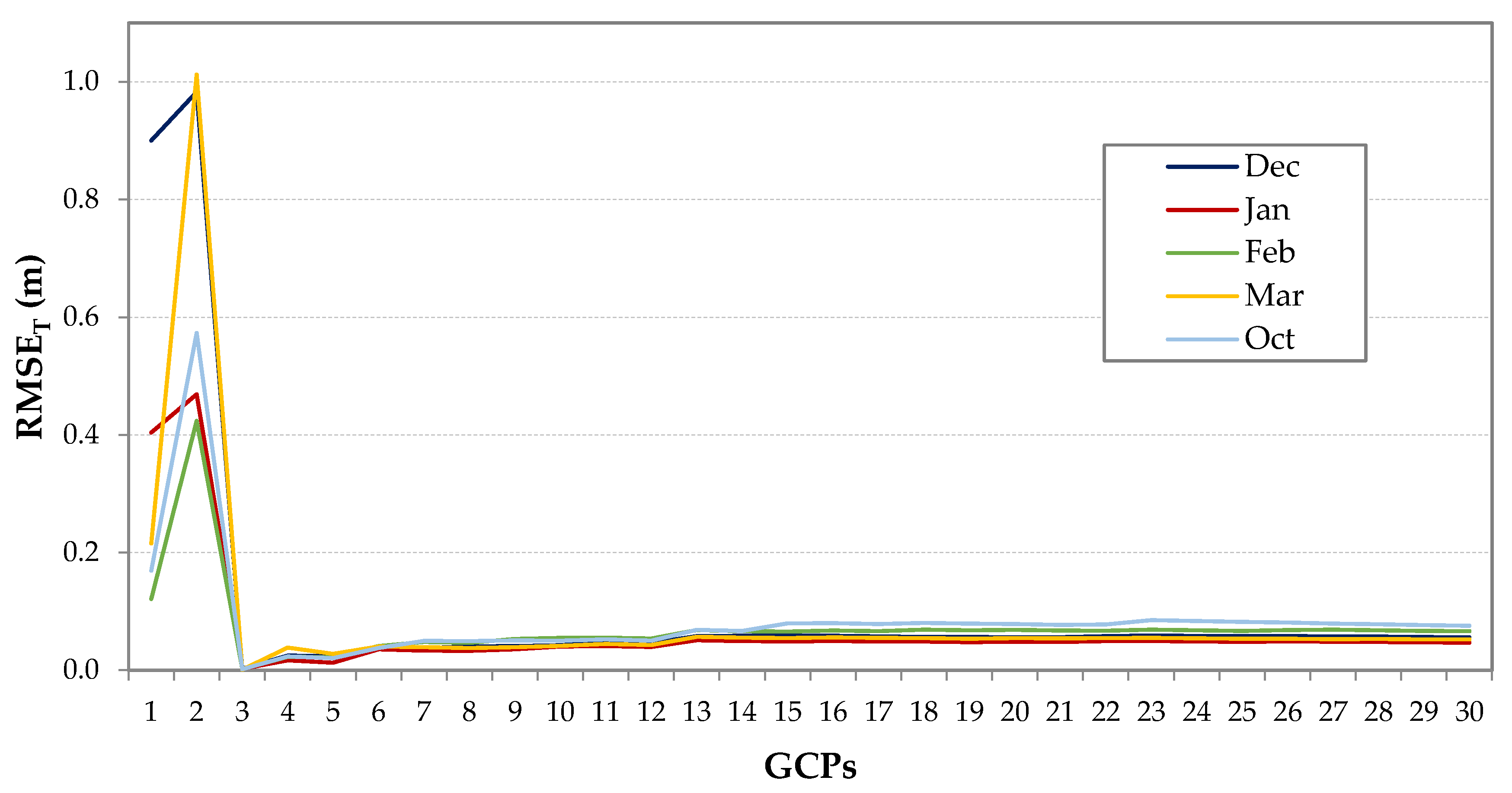
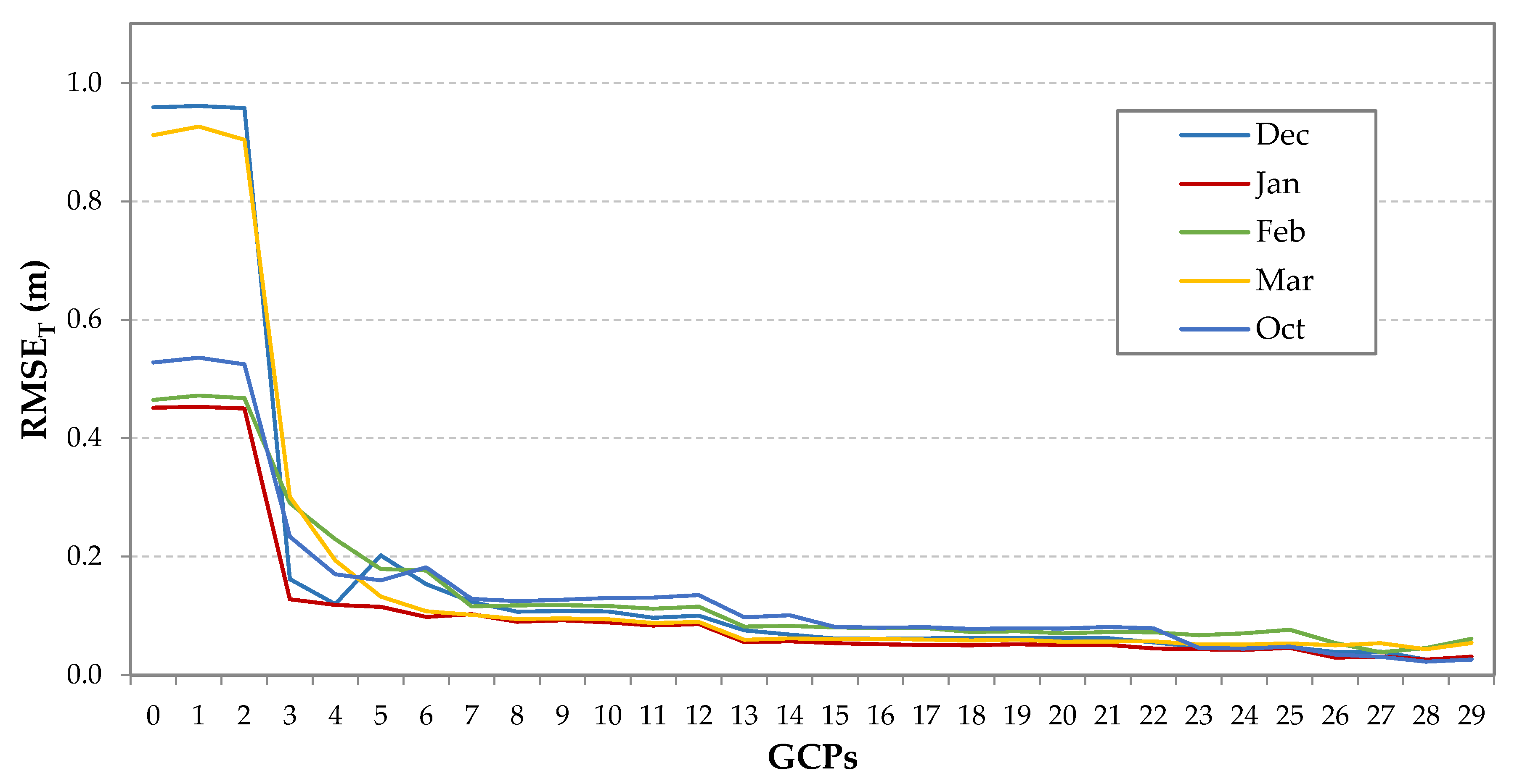
3.1. Accuracy of Photogrammetric Measurements

Suitability of available images to generate a reliable photogrammetric product was assessed through the application of the image quality tool in Agisoft PhotoScan. All images showed a satisfying value presenting an average image quality index equal to 0.8 (higher than the threshold value set to 0.5); consequently, no image was removed.

Accuracy of photogrammetric measurements were assessed with reference to RMSE_T for both GCPs and CPs. They were tested against the number of GCPs used during BBA (Figure 6 and Figure 7). Highest RMSE values (for both GCPs and CPs) correspond to the solution obtained using 1 or 2 GCPs. This confirms that, minimally 3 points are needed to properly orient a 3D model in a 3D space to recover translation, rotation and scaling values [8]. Nevertheless, the SfM/SIFT based approach can provide reasonable solutions of BBA even when GCPs number is lower than the theoretically minimum one, i.e., 3, just exploiting position and attitude data from RPAS GNSS/IMU low quality system. In spite of this interesting consideration characterizing the new digital photogrammetry, what is evident is that accuracy and processing time increases with GCPs number.

Figure 7 shows RMSE_T (for CPs) as computed while varying the number of GCPs during BBA. In this case, the CIG method is not reported. As previously, highest RMSE values were obtained when GCPs number was lower than 3, demonstrating that GNSS and IMU measures from RPAS system, in spite of their low quality, can drive to a reasonable solution (0.5–1 m) that could be accepted for many applications. This appeared to be similar for both CGPs and CPs, making those RMSE values sufficiently representative of the actual accuracy condition when working in DG mode. For the goals of this work, this fact is secondary and certainly must be overcame focusing the attention on the best expected solutions. In general, one can say that a good solution for BBA is the one when RMSE_GCP and RMSE_CP are consistent each other. With respect to Figure 6 and Figure 7 this situation occurs reaching a number of well distributed GCPs around 14. More GCPs would appear as useless.

3.2. Testing Relationship between Errors and I.O Parameters

Table 4. Statistics of I.O. parameters estimates computed with respect to the 31 repetitions for the 5 processed datasets (December 2018, January 2019, February 2019, March 2019, October 2019); Stat—statistic; Max—maximum; Min—minimum; SD—standard deviation; f—focal length; x_p and y_p coordinates of principal point; B₁; B₂—skew coefficients; K₁, K₂, K₃, K₄ —radial distortion coefficients; P₁, P₂, P₃, P₄—decentering distortion coefficients.

Survey	Stat.	f (pix)	xp (pix)	yp (pix)	B1	B2	K1	K2	K3	K4	P1	P2	P3	P4
Dec.	Max	2366.210	−0.190	6.850	2.720	0.160	−0.1300	0.1400	−0.0300	0.0140	0.0004	−0.0002	−0.0900	0.3100
	Min	2221.830	−3.200	3.480	−0.730	−0.960	−0.1400	0.1100	−0.0500	0.0084	−0.0004	−0.0008	−0.4900	0.1900
	Mean	2285.310	−2.310	4.880	0.800	−0.440	−0.1400	0.1200	−0.0400	0.0106	0.0003	−0.0005	−0.3700	0.2700
	SD	31.570	0.820	0.770	0.990	0.310	0.0000	0.0100	0.0030	0.0012	0.0002	0.0001	0.0800	0.0400
Jan.	Max	2358.480	−1.470	5.820	2.690	1.210	−0.1300	0.1400	−0.0372	0.0143	0.0007	−0.0003	−0.0018	0.3300
	Min	2262.760	−4.660	4.350	−0.030	−1.270	−0.1400	0.1200	−0.0486	0.0100	−0.0001	−0.0006	−0.5856	−0.0300
	Mean	2319.960	−3.680	5.180	0.930	−0.540	−0.1400	0.1300	−0.0433	0.0122	0.0005	−0.0005	−0.4703	0.2700
	SD	18.790	0.930	0.340	0.850	0.530	0.0000	0.0000	0.0023	0.0009	0.0002	0.0001	0.1548	0.0900
Feb.	Max	2366.490	−1.590	4.450	3.250	0.010	−0.1400	0.1400	−0.0400	0.0100	0.0004	−0.0002	0.1900	0.3300
	Min	2310.470	−2.830	3.460	0.130	−1.160	−0.1500	0.1200	−0.0500	0.0100	−0.0001	−0.0004	−0.3900	−0.0400
	Mean	2339.330	−2.190	3.780	1.150	−0.480	−0.1400	0.1300	−0.0400	0.0100	0.0003	−0.0003	−0.2500	0.2300
	SD	11.711	0.300	0.200	0.870	0.280	0.0000	0.0030	0.0010	0.0005	0.0001	0.0001	0.1550	0.0940
Mar.	Max	2320.640	2.730	7.040	2.040	1.300	−0.1300	0.1300	−0.0400	0.0100	0.0002	−0.0001	0.3600	0.5100
	Min	2267.750	−1.550	1.960	−2.690	−1.420	−0.1400	0.1200	−0.0400	0.0100	−0.0007	−0.0006	−0.4800	0.0100
	Mean	2305.520	−0.070	3.290	0.450	−0.590	−0.1400	0.1300	−0.0400	0.0100	0.0000	−0.0002	0.0300	0.3300
	SD	16.800	1.070	1.660	1.380	0.790	0.0000	0.0000	0.0016	0.0006	0.0003	0.0001	0.2300	0.1700
Oct.	Max	2363.460	−0.490	4.760	1.680	0.180	−0.1400	0.1400	−0.0400	0.0150	0.0003	−0.0003	−0.1860	0.2910
	Min	2275.080	−2.450	2.940	−1.220	−2.040	−0.1600	0.1200	−0.0500	0.0110	−0.0003	−0.0007	−0.4720	0.1190
	Mean	2338.246	−1.650	3.790	0.220	−0.990	−0.1400	0.1340	−0.0470	0.0140	0.0002	−0.0004	−0.3010	0.2260
	SD	26.293	0.530	0.520	0.750	0.570	0.0000	0.0060	0.0030	0.0010	0.0002	0.0001	0.0830	0.0630

reports the main statistics computed for all the estimated I.O. parameters with respect to all processed dataset. It can be noted that I.O. parameters can be grouped in two clusters: one including x_p, y_p, B₁, B₂, P₃ and P₄ is characterized by a great variability; another one, including remaining parameters, shows pretty similar values for all the computed metrics. Since all trials generated similar estimates of radial and tangential distortion parameters, these can be retained strictly dependent on the camera with no conditioning by other factors. Moreover, P_i coefficients are known to be less significant than radial ones (one or two orders of magnitude smaller [59]). Boxplots of Figures 9–13 confirm this fact.

A further synthetic analysis can come from the coefficient of variation (CV = standard deviation/mean × 100.0, %) of I.O. parameters estimates. Results are reported in Figure 8. It can be noted that focal length f and K_i coefficients are the most stables parameters. Conversely, x_p, y_p, B_i and P_i coefficients present a wide variability depending on operational conditions.

According to the boxplots of Figure 9, Figure 10, Figure 11, Figure 12 and Figure 13 a similar trend can be recognized affecting all I.O. parameters. Specifically, the October dataset (Figure 13) appears to not contain any outlier for the most of parameters (f, K₁–K₂–K₃–K₄–P₃–P₄). Oppositely, in the other datasets no outlier was found for B₁, P₁, P₂ in the December dataset (Figure 9); y_p and x_p did not present outliers in the January and February datasets (Figure 10 and Figure 11); f, P₄ and K₂ had no outliers in the March dataset (Figure 12).

The relationships among I.O. parameters were explored by computing the correlation matrices for all the datasets. Results are reported in

Table 5. Correlation matrix of camera I.O. parameters as estimated from the December 2018 dataset (f—focal length; x_p and y_p coordinates of the principal point offset; B₁, B₂—skew parameters; K₁, K₂, K₃, K₄—radial distortions; P₁, P₂, P₃, P₄—components of the decentering distortions).

	f (pix)	xp (pix)	yp (pix)	B1	B2	K1	K2	K3	K4	P1	P2	P3	P4
f (pix)	1.00	−0.15	−0.56	0.10	0.03	−1.00	1.00	−1.00	0.99	0.27	0.51	0.37	0.44
xp (pix)	−0.15	1.00	0.51	−0.26	−0.04	0.12	−0.12	0.08	−0.07	−0.96	−0.58	0.43	−0.73
yp (pix)	−0.56	0.51	1.00	−0.49	0.29	0.54	−0.55	0.53	−0.53	−0.69	−0.91	−0.48	−0.43
B1	0.10	−0.26	−0.49	1.00	−0.59	−0.06	0.12	−0.08	0.10	0.35	0.20	0.44	−0.17
B2	0.03	−0.04	0.29	−0.59	1.00	−0.04	0.02	−0.04	0.03	−0.12	−0.02	−0.37	0.12
K1	−1.00	0.12	0.54	−0.06	−0.04	1.00	−1.00	1.00	−1.00	−0.23	−0.51	−0.38	−0.42
K2	1.00	−0.12	−0.55	0.12	0.02	−1.00	1.00	−1.00	1.00	0.24	0.50	0.40	0.41
K3	−1.00	0.08	0.53	−0.08	−0.04	1.00	−1.00	1.00	−1.00	−0.20	−0.49	−0.42	−0.38
K4	0.99	−0.07	−0.53	0.10	0.03	−1.00	1.00	−1.00	1.00	0.19	0.48	0.43	0.37
P1	0.27	−0.96	−0.69	0.35	−0.12	−0.23	0.24	−0.20	0.19	1.00	0.68	−0.26	0.78
P2	0.51	−0.58	−0.91	0.20	−0.02	−0.51	0.50	−0.49	0.48	0.68	1.00	0.31	0.49
P3	0.37	0.43	−0.48	0.44	−0.37	−0.38	0.40	−0.42	0.43	−0.26	0.31	1.00	−0.46
P4	0.44	−0.73	−0.43	−0.17	0.12	−0.42	0.41	−0.38	0.37	0.78	0.49	−0.46	1.00

,

Table 6. Correlation matrix of camera I.O. parameters as estimated from the January 2019 dataset (f—focal length; x_p and y_p coordinates of the principal point offset; B₁, B₂—skew parameters; K₁, K₂, K₃, K₄—radial distortions; P₁, P₂, P₃, P₄—components of the decentering distortions).

	f (pix)	xp (pix)	yp (pix)	B1	B2	K1	K2	K3	K4	P1	P2	P3	P4
f (pix)	1	0.51	−0.30	−0.27	0.59	−1.00	1.00	−0.99	0.98	−0.52	−0.17	0.55	−0.52
xp (pix)	0.51	1	−0.46	−0.02	0.72	−0.52	0.57	−0.63	0.65	−0.98	−0.36	0.95	−0.92
yp (pix)	−0.30	−0.46	1	0.43	−0.25	0.32	−0.30	0.32	−0.32	0.35	−0.37	−0.55	0.44
B1	−0.27	−0.02	0.43	1	−0.39	0.27	−0.25	0.29	−0.29	0.08	0.04	−0.24	0.18
B2	0.59	0.72	−0.25	−0.39	1	−0.60	0.64	−0.70	0.72	−0.81	−0.21	0.83	−0.87
K1	−1.00	−0.52	0.32	0.27	−0.60	1	−1.00	0.99	−0.98	0.54	0.15	−0.57	0.54
K2	1.00	0.57	−0.30	−0.25	0.64	−1.00	1	−0.99	0.99	−0.58	−0.19	0.60	−0.58
K3	−0.99	−0.63	0.32	0.29	−0.70	0.99	−0.99	1	−1.00	0.65	0.23	−0.67	0.65
K4	0.98	0.65	−0.32	−0.29	0.72	−0.98	0.99	−1.00	1	−0.67	−0.25	0.69	−0.67
P1	−0.52	−0.98	0.35	0.08	−0.81	0.54	−0.58	0.65	−0.67	1	0.43	−0.95	0.95
P2	−0.17	−0.36	−0.37	0.04	−0.21	0.15	−0.19	0.23	−0.25	0.43	1	−0.24	0.22
P3	0.55	0.95	−0.55	−0.24	0.83	−0.57	0.60	−0.67	0.69	−0.95	−0.24	1	−0.98
P4	−0.52	−0.92	0.44	0.18	−0.87	0.54	−0.58	0.65	−0.67	0.95	0.22	−0.98	1

,

Table 7. Correlation matrix of camera I.O. parameters as estimated from the February 2019 dataset (f—focal length; x_p and y_p coordinates of the principal point offset; B₁, B₂—skew parameters; K₁, K₂, K₃, K₄—radial distortions; P₁, P₂, P₃, P₄—components of the decentering distortions).

	f (pix)	xp (pix)	yp (pix)	B1	B2	K1	K2	K3	K4	P1	P2	P3	P4
f (pix)	1	0.008	0.18	0.16	−0.16	−0.88	0.99	−0.93	0.97	0.14	−0.15	−0.12	0.19
xp (pix)	0.01	1	−0.51	0.18	−0.34	−0.35	0.12	−0.27	0.20	−0.77	0.26	0.74	−0.56
yp (pix)	0.18	−0.51	1	0.48	0.08	−0.09	0.18	−0.14	0.18	0.18	−0.40	−0.33	0.19
B1	0.16	0.18	0.48	1	−0.32	−0.14	0.20	−0.16	0.19	−0.04	0.16	−0.17	0.22
B2	−0.16	−0.34	0.08	−0.32	1	0.15	−0.18	0.18	−0.20	0.05	−0.01	−0.01	−0.03
K1	−0.88	−0.35	−0.09	−0.14	0.15	1	−0.93	0.99	−0.95	0.27	0.09	−0.27	0.17
K2	0.99	0.12	0.18	0.20	−0.18	−0.93	1	−0.97	0.99	0.01	−0.14	−0.01	0.08
K3	−0.93	−0.27	−0.14	−0.16	0.18	0.99	−0.97	1	−0.99	0.19	0.14	−0.18	0.10
K4	0.97	0.20	0.18	0.19	−0.20	−0.95	0.99	−0.99	1	−0.09	−0.16	0.08	−0.01
P1	0.14	−0.77	0.18	−0.04	0.05	0.27	0.01	0.19	−0.09	1	0.11	−0.94	0.90
P2	−0.15	0.26	−0.40	0.16	−0.01	0.09	−0.14	0.14	−0.16	0.11	1	−0.27	0.43
P3	−0.12	0.74	−0.33	−0.17	−0.01	−0.27	−0.01	−0.18	0.08	−0.94	−0.27	1	−0.97
P4	0.19	−0.56	0.19	0.22	−0.03	0.17	0.08	0.10	−0.01	0.90	0.43	−0.97	1

,

Table 8. Correlation matrix of camera I.O. parameters as estimated from the March 2019 dataset (f—focal length; x_p and y_p coordinates of the principal point offset; B₁, B₂—skew parameters; K₁, K₂, K₃, K₄—radial distortions; P₁, P₂, P₃, P₄—components of the decentering distortions).

	f (pix)	xp (pix)	yp (pix)	B1	B2	K1	K2	K3	K4	P1	P2	P3	P4
f (pix)	1.00	0.04	−0.70	0.13	−0.40	−0.95	1.00	−0.94	0.96	0.53	0.77	0.66	0.78
xp (pix)	0.04	1.00	0.49	−0.94	0.76	−0.31	0.10	−0.32	0.28	−0.73	−0.30	−0.38	0.06
yp (pix)	−0.70	0.49	1.00	−0.66	0.85	0.46	−0.64	0.43	−0.47	−0.94	−0.93	−0.93	−0.81
B1	0.13	−0.94	−0.66	1.00	−0.90	0.16	0.06	0.18	−0.13	0.85	0.50	0.58	0.12
B2	−0.40	0.76	0.85	−0.90	1.00	0.14	−0.34	0.10	−0.14	−0.91	−0.70	−0.78	−0.45
K1	−0.95	−0.31	0.46	0.16	0.14	1.00	−0.97	1.00	−0.99	−0.25	−0.60	−0.45	−0.69
K2	1.00	0.10	−0.64	0.06	−0.34	−0.97	1.00	−0.97	0.98	0.46	0.73	0.61	0.75
K3	−0.94	−0.32	0.43	0.18	0.10	1.00	−0.97	1.00	−1.00	−0.22	−0.57	−0.42	−0.65
K4	0.96	0.28	−0.47	−0.13	−0.14	−0.99	0.98	−1.00	1.00	0.27	0.60	0.46	0.67
P1	0.53	−0.73	−0.94	0.85	−0.91	−0.25	0.46	−0.22	0.27	1.00	0.85	0.84	0.61
P2	0.77	−0.30	−0.93	0.50	−0.70	−0.60	0.73	−0.57	0.60	0.85	1.00	0.85	0.81
P3	0.66	−0.38	−0.93	0.58	−0.78	−0.45	0.61	−0.42	0.46	0.84	0.85	1.00	0.78
P4	0.78	0.06	−0.81	0.12	−0.45	−0.69	0.75	−0.65	0.67	0.61	0.81	0.78	1.00

and

Table 9. Correlation matrix of camera I.O. parameters as estimated from the October 2019 dataset (f—focal length; x_p and y_p coordinates of the principal point offset; B₁, B₂—skew parameters; K₁, K₂, K₃, K₄—radial distortions; P₁, P₂, P₃, P₄—components of the decentering distortions).

	f (pix)	xp (pix)	yp (pix)	B1	B2	K1	K2	K3	K4	P1	P2	P3	P4
f (pix)	1.00	−0.63	−0.50	−0.26	−0.26	−1.00	1.00	−1.00	1.00	0.70	0.51	−0.54	0.83
xp (pix)	−0.63	1.00	0.28	−0.28	0.30	0.58	−0.63	0.60	−0.62	−0.91	−0.66	0.73	−0.65
yp (pix)	−0.50	0.28	1.00	0.01	0.13	0.46	−0.49	0.47	−0.48	−0.63	−0.77	−0.28	−0.43
B1	−0.26	−0.28	0.01	1.00	−0.64	0.31	−0.26	0.28	−0.27	0.27	0.42	0.12	−0.41
B2	−0.26	0.30	0.13	−0.64	1.00	0.23	−0.27	0.25	−0.26	−0.35	−0.38	0.10	0.04
K1	−1.00	0.58	0.46	0.31	0.23	1.00	−1.00	1.00	−1.00	−0.65	−0.46	0.53	−0.81
K2	1.00	−0.63	−0.49	−0.26	−0.27	−1.00	1.00	−1.00	1.00	0.70	0.50	−0.54	0.82
K3	−1.00	0.60	0.47	0.28	0.25	1.00	−1.00	1.00	−1.00	−0.67	−0.48	0.54	−0.82
K4	1.00	−0.62	−0.48	−0.27	−0.26	−1.00	1.00	−1.00	1.00	0.69	0.49	−0.55	0.82
P1	0.70	−0.91	−0.63	0.27	−0.35	−0.65	0.70	−0.67	0.69	1.00	0.83	−0.47	0.71
P2	0.51	−0.66	−0.77	0.42	−0.38	−0.46	0.50	−0.48	0.49	0.83	1.00	−0.04	0.32
P3	−0.54	0.73	−0.28	0.12	0.10	0.53	−0.54	0.54	−0.55	−0.47	−0.04	1.00	−0.65
P4	0.83	−0.65	−0.43	−0.41	0.04	−0.81	0.82	−0.82	0.82	0.71	0.32	−0.65	1.00

. The correlation matrix contains positive and negative values in the range [−1, +1]. Positive values mean that a direct relationship between variables is present; negative values an inverse linkage. The higher the values, the stronger the correlation. All the datasets showed pretty similar values, that can be synthesized as it follows: focal length was highly correlated with radial aberrations coefficients; x_p was moderately correlated with y_p and, in the most of cases, with P_i coefficients; y_p was poorly/moderately correlated with all the other parameters (March dataset excluded); skew parameters (B₁,B₂) were poorly/moderately correlated with the other parameters (March dataset excluded); K_i coefficients showed to be internally correlated each other and, externally, with the focal length; a moderate correlation was found between y_p and P₂. January and February dataset showed low correlation between K_i with y_p and P₂. In spite of all specific situations, these results suggested that I.O. parameters contain redundant information. Consequently, a PCA was operated showing that the most of the decorrelated information could be explained by few PCs, whose identification was operated by Kaiser’s criterion.

The errors affecting final measures from oriented image blocks were evaluated with reference to the above mentioned RMSE_j. Analysis was separately performed for both GCPs and CPs and for all the datasets (

Table 10. Statistics about error components computed with reference to GCPs and CPs RMSE_j for all tested datasets (Dec.—December; Jan.—January; Feb.—February; Mar.—March; Oct.—October; E—East coordinate; N—North coordinate; H—height coordinate; T—3D error; I—positioning error in the image space; Max; Min—minimum; SD—standard deviation).

Survey	Statistics	GCPs					CPs
		RMSEE (m)	RMSEN (m)	RMSEH (m)	RMSET (m)	RMSEI (pix)	RMSEE (m)	RMSEN (m)	RMSEH (m)	RMSET (m)	RMSEI (pix)
Dec.	Max	0.20	0.09	0.96	0.98	0.27	0.21	0.09	0.93	0.96	0.27
	Min	0.00	0.00	0.00	0.00	0.18	0.01	0.02	0.00	0.03	0.19
	Mean	0.04	0.02	0.09	0.11	0.25	0.07	0.04	0.14	0.17	0.25
	SD	0.04	0.02	0.23	0.23	0.03	0.05	0.02	0.27	0.27	0.03
Jan.	Max	0.11	0.090	0.45	0.47	0.27	0.130	0.109	0.421	0.453	0.311
	Min	0.002	0.0012	0.00018	0.0023	0.20	0.011	0.020	0.010	0.026	0.220
	Mean	0.035	0.025	0.044	0.068	0.24	0.052	0.043	0.070	0.104	0.237
	SD	0.019	0.016	0.10	0.10	0.016	0.035	0.026	0.119	0.121	0.019
Feb.	Max	0.20	0.22	0.31	0.42	0.31	0.21	0.21	0.37	0.47	0.22
	Min	0.0017	0.0011	0.0006	0.0022	0.21	0.02	0.03	0.02	0.04	0.17
	Mean	0.033	0.045	0.044	0.072	0.23	0.06	0.07	0.10	0.14	0.21
	SD	0.033	0.035	0.051	0.069	0.023	0.054	0.051	0.103	0.124	0.010
Mar.	Max	0.461	0.259	0.863	1.012	0.273	0.451	0.221	0.778	0.926	0.360
	Min	0.0005	0.001	0.000	0.001	0.110	0.028	0.027	0.018	0.044	0.243
	Mean	0.057	0.030	0.048	0.085	0.236	0.094	0.056	0.117	0.166	0.266
	SD	0.083	0.044	0.154	0.178	0.032	0.122	0.057	0.225	0.259	0.023
Oct.	Max	0.306	0.129	0.467	0.573	0.234	0.304	0.114	0.426	0.536	0.278
	Min	0.001	0.001	0.001	0.002	0.182	0.005	0.002	0.020	0.023	0.221
	Mean	0.055	0.030	0.055	0.085	0.222	0.089	0.034	0.101	0.140	0.235
	SD	0.051	0.024	0.080	0.097	0.015	0.081	0.030	0.113	0.141	0.011

). It showed similar values for all the datasets. RMSE_I defines the reprojection error computed as the mean distance (in the image space) between the position expected for a tie point that participated to solve block orientation and the one resulting by reprojection of the correspondent 3D object point after image resection. To minimize alignment issues, the maximum values of error should be <1, according to [44]. This condition was respected for all the blocks: the maximum detected value was 0.31 and 0.36 for GCPs an CPs (

Table 11. Correlation matrix of error components computed from RMSE_GCP and RMSE_CPs for each acquired dataset (Dec.—December; Jan.—January; Feb.—February; Mar.—March; Oct.—October; E—East coordinate; N—North coordinate; H—height coordinate; T—3D error; I—positioning error).

Survey	Error Components	GCPs					CPs
		RMSEE	RMSEN	RMSEH	RMSET	RMSEI	RMSEE	RMSEN	RMSEH	RMSET	RMSEI
Dec.	RMSEE	1	0.813	0.894	0.906	−0.033	1	0.929	0.918	0.932	0.530
	RMSEN	0.813	1	0.884	0.894	0.072	0.929	1	0.952	0.957	0.292
	RMSEH	0.894	0.884	1	0.999	−0.283	0.918	0.952	1	0.999	0.227
	RMSET	0.906	0.894	0.999	1	−0.258	0.932	0.957	0.999	1	0.254
	RMSEI	−0.033	0.072	−0.283	−0.258	1	0.530	0.292	0.227	0.254	1
Jan.	RMSEE	1	0.88	0.82	0.85	−0.06	1	0.95	0.80	0.87	−0.13
	RMSEN	0.88	1	0.96	0.97	−0.27	0.95	1	0.89	0.95	−0.02
	RMSEH	0.82	0.96	1	1.00	−0.33	0.80	0.89	1	0.99	0.03
	RMSET	0.85	0.97	1.00	1	−0.33	0.87	0.95	0.99	1	−0.002
	RMSEI	−0.06	−0.27	−0.33	−0.33	1	−0.13	−0.02	0.03	−0.002	1
Feb.	RMSEE	1	0.96	0.96	0.98	−0.08	1	0.97	0.91	0.95	0.31
	RMSEN	0.96	1	0.99	1.00	0.07	0.97	1	0.94	0.98	0.27
	RMSEH	0.96	0.99	1	1.00	0.12	0.91	0.94	1	0.99	0.27
	RMSET	0.98	1.00	1.00	1	0.07	0.95	0.98	0.99	1	0.28
	RMSEI	−0.08	0.07	0.12	0.07	1	0.31	0.27	0.27	0.28	1
Mar.	RMSEE	1.00	0.94	0.94	0.98	−0.64	1.00	0.97	0.99	0.99	−0.34
	RMSEN	0.94	1.00	1.00	0.99	−0.44	0.97	1.00	1.00	0.99	−0.26
	RMSEH	0.94	1.00	1.00	0.99	−0.45	0.99	1.00	1.00	1.00	−0.27
	RMSET	0.98	0.99	0.99	1.00	−0.53	0.99	0.99	1.00	1.00	−0.29
	RMSEI	−0.64	−0.44	−0.45	−0.53	1.00	−0.34	−0.26	−0.27	−0.29	1.00
Oct.	RMSEE	1.00	0.89	0.99	0.99	−0.07	1.00	0.98	0.96	0.99	−0.16
	RMSEN	0.89	1.00	0.87	0.90	−0.08	0.98	1.00	0.97	0.99	−0.19
	RMSEH	0.99	0.87	1.00	1.00	−0.20	0.96	0.97	1.00	0.99	−0.14
	RMSET	0.99	0.90	1.00	1.00	−0.16	0.99	0.99	0.99	1.00	−0.15
	RMSEI	−0.07	−0.08	−0.20	−0.16	1.00	−0.16	−0.19	−0.14	−0.15	1.00

), respectively. Conversely, RMSE_N, RMSE_H, RMSE_T define the distance (in the object space) between the expected position of a GCP (or CP) and the one determined by photogrammetric measurement in the object space. The smaller this value, the higher the final accuracy. These parameters are known to be strongly influenced by user’s experience in recognizing the proper markers (shape, color, stability, etc.) within image and operate the correspondent collimation. The highest RMSE_T values were detected in the December (0.98 m) and March (1.01 m) datasets.

The correlation matrices were computed to analyze possible relationships among error components for both GCPs and CPs (Figure 10 and Figure 11). Results showed a high direct correlation among all the variables, reprojection error excluded (RMSE_I).

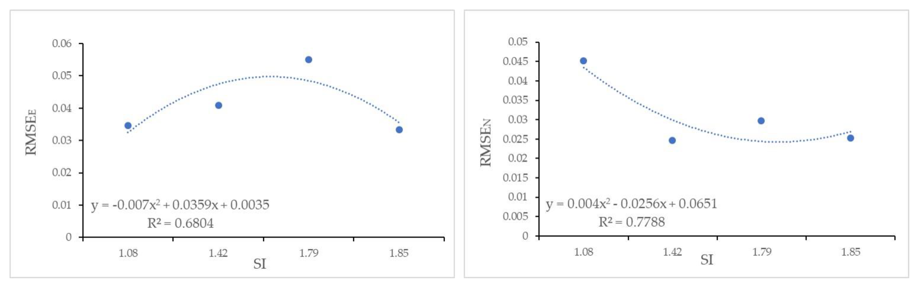
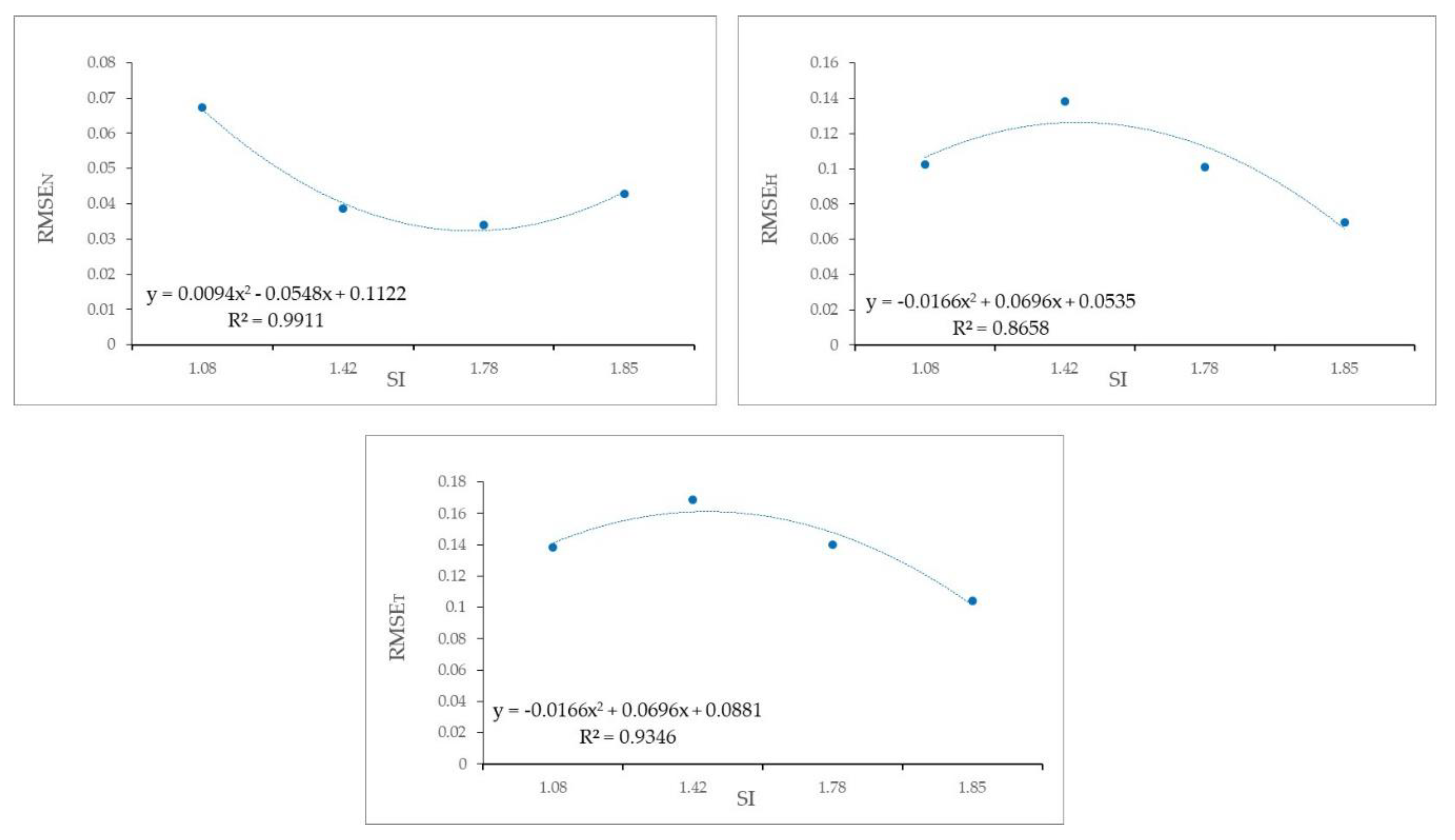
3.3. Calibrating Predictive Models

Camera I.O. parameters estimates were analyzed by PCA to detect and remove redundant information. As usual, December, January, February and October blocks were separately processed to identify those PCs that, for each dataset, could synthesize the most of the original information. This was done with reference to the correlation plots relating I.O. parameters with PC (Figure 14). Application of Kaiser’s criterion showed that the strongest three PCs were enough to describe the most of I.O. parameters variance for the December (Figure 14a), January (Figure 14b) and October (Figure 14d) datasets. Conversely, five PCs were needed to explain the most of information resident in I.O parameters estimates from the February dataset (Figure 14c). These results confirmed what base statistics of Table 5, Table 6, Table 7, Table 8 and Table 9 had already shown: I.O. parameters are highly intracorrelated.

The most significant PCs, as resulting from the previous analysis, were aggregated by Equation (4) to compute SI that was used as predictor within the predictive functions of RMSE. SI values are reported in

Table 12. Synthetic index (SI) as computed by Equation (4) for the December, January, February and October datasets.

Variable	December	January	February	October
SI	1.42	1.85	1.08	1.79

. Before calibrating predictive functions possibly relating SI to RMSE the Pearson’s coefficient was computed between SI and all the available RMSE for both GCPs and CPs (

Table 13. Correlation coefficient between RMSE_j and SI computed for each dataset (GCPs = ground control points; CPs = check points; E = East coordinate; N = North coordinate; H = height coordinate; T = 3D error; I = positioning error in the image space).

	GCPs					CPs
	RMSEE	RMSEN	RMSEH	RMSET	RMSEI	RMSEE	RMSEN	RMSEH	RMSET	RMSEI
Pearson’s R	0.5	−0.8	−0.10	−0.12	−0.11	0.28	−0.80	−0.50	−0.49	0.67

).

Only situations showing a moderate (0.5 < R < 0.7) or a high Pearson’s coefficient (>0.7) were modeled in the following step [71]. Consequently, since SI showed a moderate and high correlation with GCPs RMSE_E and RMSE_N, respectively these relationships were modeled. Conversely, since CPs RMSE_E showed a low correlation with SI it was excluded from modeling.

A 2nd order polynomial showed to better fit the data. Results concerning GCPs and CPs are shown in Figure 15 and Figure 16, respectively. Graphs also report the coefficient of determination (R²). For GCPs, the lowest R² value was 0.68 (RMSE_E), while CPs RMSE_N showed the highest R² (0.99).

Table 14. Coefficients of the calibrated predictive functions (E—East coordinate; N—North coordinate; H—height coordinate; T—total (3D) error; I—positioning error in the image space).

	RMSEE (M)– GCPS	RMSEN (M)– GCPS	RMSEN (M)– CPS	RMSEH (M)– CPS	RMSET (PIX)– CPS
a	−0.0070	0.0040	0.0094	−0.0166	−0.0166
b	0.0359	−0.0256	−0.0548	0.0696	0.0696
c	0.0035	0.0651	0.1122	0.0535	0.0881

reports the coefficients of the significant 2nd order polynomial predictive functions for both CPs and GCPs.

3.4. Validating Predictive Models

Reliability and accuracy of the proposed predictive method were tested by applying the calibrated models to all the available datasets, March included. With respect to March dataset specifically, PCA analysis was applied to recognize significant PCs able to explain the most of I.O. parameters variance. Two PCs were found to satisfy the Kaiser’s criterion and, consequently, they were used to compute March SI (3.060). March SI value was then used to predict RMSEj according to Equation (5) applied using the coefficients from Table 14. To summarize performances of models, all the RMSEj estimates were compared, by differencing, with the correspondent values from the BBA solutions (reference ones). RMSE was then computed for all the tested differences and estimated RMSEj. Results are reported in

Table 15. Differences between RMSE_j values as estimated by the calibrated predictive models and the correspondent ones from BBA for the March dataset.

Errors	March Dataset Difference (m)
RMSEE (GCPs)	0.0024
RMSEN (GCPs)	0.0047
RMSEN (CPs)	0.0110
RMSEH (CPs)	0.0039
RMSEI (CPs)	0.0014

.

4. Discussion

This research was intended to explore dependency of the accuracy of measures from RPAS-based SfM 3D models from the camera I.O. parameters estimates. Several researchers investigated these issue, detecting the strong influence of camera parameters on final accuracy of obtainable measures. Nevertheless, no proposal came for an operative procedure able to predict the potential achievable accuracy once camera parameters were known. In this work, authors tried to fill this gap by developing and proposing a simple method that, in their preliminary tests, provided promising results. The proposed approach integrates uni- and multivariate statistics to investigate and removing correlated information resident in I.O. parameters of the camera as estimated during BBA.

The study was based on five photogrammetric surveys by RPAS operated in December 2018 and January, February, March and October of 2019 (Table 1). A ground survey campaign was also done to position 30 well distributed GCPs. All flight missions were performed by DJI Inspire 1 drone, equipped with DJI ZenMuse X3 camera. To ensure comparability of datasets all missions were operated according to the same flight plan (path, speed and height) and BBA was performed setting the same parameters within Agisoft PhotoScan. The same skilled user was in charge of processing data and optimizing the photogrammetric solution.

A first step was aimed at testing image blocks quality and removing “bad” images. A second step was aimed at solving BBA iteratively changing the number of GCPs. A total of 155 chunks (31 chunks for each mission) were analyzed. It is worth to remind that this step was not aimed at selecting the best spatial strategy for positioning GCPs; differently, it was devoted to evaluating the achievable accuracy of final measures and the accuracy dependence on GCPs number. As shown in Figure 6 and Figure 7, highest RMSE_T correspond to those solutions were direct georeferencing plays the leading role, being the number of GCPs lower than the theoretical minimum value (3, [8]). By comparing GCPs and CPs RMSE_T trend with the number of GCPs it was found that the optimal minimum number of GCPs was around 14 (Figure 6 and Figure 7). All the datasets showed the same GCPs and CPs RMSE_T trend. Just few dissimilarities were found, probably due to different environmental conditions (e.g., lighting, weather conditions, vegetation phenology). After this preliminary investigation that ensured about comparability of processed datasets, a deeper investigation concerned errors components separately (RMSE_j). Some basic statistics (e.g., maximum, minimum, mean and standard deviation) of I.O. parameters estimates were also computed for each processed dataset (Table 10). All of them showed similar statistics. Results confirmed what reported in previous works: Agisoft PhotoScan, as well as other photogrammetric software, in general, cannot estimate stable I.O. parameters while initial conditions (e.g., GCPs number) change [29,59]. In fact, stats showed a high variability of solutions. Nevertheless, the order of magnitude remained the same in all dataset (Table 4) and a similar trend, as shown in the boxplots of Figure 9, Figure 10, Figure 11, Figure 12 and Figure 13. Moreover, the obtained order of magnitude is coherent with the one obtained by other researchers [59]; they showed that P_i parameters are smaller by one or two orders of magnitude than radial ones and that K_i present the most significant deviations.

Correlations among I.O. parameters was then investigated finding a high degree of intracorrelation. Correlation values proved to be consistent with those reported in literature (Table 5, Table 6, Table 7, Table 8 and Table 9 [59]). Correlated information was aggregated by PCA [60]; it was found that from two to five PCs are generally enough to explain the most of variance of I.O. parameters estimates.

With these premises, an index (SI) was defined to summarize the decorrelated information that the first PCs were able to aggregate. SI was assumed as predictor of RMSE_j and correspondent predictive function calibrated (Figure 15 and Figure 16). Models calibration was obtained with reference to the December, January, February and October datasets. March dataset was differently used to validate predictive models.

In spite of the few observations used for calibration, the proposed predictive functions showed satisfying results when applied to the validation set generating RMSE_j estimates very close to the actual values as computed during BBA by Agisoft PhotoScan. Results are must be assumed as preliminary, but certainly encouraging.

5. Conclusions

The present study was aimed at exploring the impact of the camera I.O. parameters on the accuracy of final photogrammetric 3D models. The possibility of calibrating predictive models for error estimates once given I.O. parameters estimates was the focus point of this research. The proposed procedure was tested on the study area of Torre a Mare (Apulian Region) through the acquisition of five photogrammetric datasets operated at different dates along the year.

After investigating image quality and achieved BBA, resulting camera I.O. parameters were explored to test their eventual intracorrelation and potential relationships with the accuracy of final photogrammetric measures. A high correlation among the most of parameters was found and a high level of information reduction can be achieved by PCA. Tests proved that from two up to five PCs are enough to explain the most of I.O. parameters variance. PCs selection was operated according to the Kaiser’s criterion. The strongest PCs—if properly aggregated along SI—showed that they are able to predict final errors in photogrammetric measures. The SI was, in fact, found to be a good predictor of errors when included, as independent variable, within a 2nd order polynomial function. Predictive functions dependent on SI were applied to all datasets included the validation one of March, obtaining satisfying predicted results as shown in Table 15.

Although the proposed method seems promising and predictive functions estimates satisfying, further investigations must be done, with the man aim of improving generalization capability of models and testing their dependencies on other operational conditions like different areas, oblique acquisitions and GCP spatial distribution.

References

1. Gold, D.P.; Parizek, R.R.; Alexander, S.A. Analysis and application of ERTS-1 data for regional geological mapping. In Proceedings of the First Symposium of Significant Results obtained from the Earth Resources Technology Satellite-1, NASA, New Carrollton, MD, USA, 5–9 March 1973; Volume 1, pp. 231–246. [Google Scholar]
2. Hooke, J.M.; Horton, B.P.; Moore, J.; Taylor, M.P. Upper river Severn (Caersws) channel study. In Report to the Countryside Council for Wales; University of Portsmouth: Portsmouth, UK, 1994. [Google Scholar]
3. Evans, I.S. World-wide variations in the direction and concentration of cirque and glacier aspects. Geogr. Ann. Ser. A Phys. Geogr. 1977, 59, 151–175. [Google Scholar] [CrossRef]
4. Drăguț, L.; Eisank, C. Object representations at multiple scales from digital elevation models. Geomorphology 2011, 129, 183–189. [Google Scholar] [CrossRef] [PubMed] [Green Version]
5. Capolupo, A.; Pindozzi, S.; Okello, C.; Boccia, L. Indirect field technology for detecting areas object of illegal spills harmful to human health: Application of drones, photogrammetry and hydrological models. Geospat. Heal. 2014, 8, 699. [Google Scholar] [CrossRef] [PubMed] [Green Version]
6. Medjkane, M.; Maquaire, O.; Costa, S.; Roulland, T.; Letortu, P.; Fauchard, C.; Antoine, R.; Davidson, R. High-resolution monitoring of complex coastal morphology changes: Cross-efficiency of SfM and TLS-based survey (Vaches-Noires cliffs, Normandy, France). Landslides 2018, 15, 1097–1108. [Google Scholar] [CrossRef]
7. Rieke-Zapp, D.H.; Wegmann, H.; Santel, F.; Nearing, M.A. Digital photogrammetry for measuring soil surface roughness. In Proceedings of the American Society of Photogrammetry & Remote Sensing 2001 Conference–Gateway to the New Millennium’, St Louis, MO, USA, 23–27 April 2001; American Society of Photogrammetry & Remote Sensing: Bethesda, MD, USA, 2001. [Google Scholar]
8. Nex, F.; Remondino, F. UAV for 3D mapping applications: A review. Appl. Geomatics 2013, 6, 1–15. [Google Scholar] [CrossRef]
9. Salamí, E.; Barrado, C.; Pastor, E. UAV Flight Experiments Applied to the Remote Sensing of Vegetated Areas. Remote Sens. 2014, 6, 11051–11081. [Google Scholar] [CrossRef] [Green Version]
10. Capolupo, A.; Pindozzi, S.; Okello, C.; Fiorentino, N.; Boccia, L. Photogrammetry for environmental monitoring: The use of drones and hydrological models for detection of soil contaminated by copper. Sci. Total. Environ. 2015, 514, 298–306. [Google Scholar] [CrossRef]
11. Manfreda, S.; McCabe, M.F.; Miller, P.E.; Lucas, R.M.; Madrigal, V.P.; Mallinis, G.; Ben Dor, E.; Helman, D.; Estes, L.; Ciraolo, G.; et al. On the Use of Unmanned Aerial Systems for Environmental Monitoring. Remote Sens. 2018, 10, 641. [Google Scholar] [CrossRef] [Green Version]
12. Capolupo, A.; Nasta, P.; Palladino, M.; Cervelli, E.; Boccia, L.; Romano, N. Assessing the ability of hybrid poplar for in-situ phytoextraction of cadmium by using UAV-photogrammetry and 3D flow simulator. Int. J. Remote. Sens. 2018, 39, 5175–5194. [Google Scholar] [CrossRef]
13. Palladino, M.; Nasta, P.; Capolupo, A.; Romano, N. Monitoring and modelling the role of phytoremediation to mitigate non-point source cadmium pollution and groundwater contamination at field scale. Ital. J. Agron. 2018, 13, 59–68. [Google Scholar]
14. Capolupo, A.; Kooistra, L.; Boccia, L. A novel approach for detecting agricultural terraced landscapes from historical and contemporaneous photogrammetric aerial photos. Int. J. Appl. Earth Obs. Geoinf. 2018, 73, 800–810. [Google Scholar] [CrossRef]
15. Cramer, M.; Przybilla, H.-J.; Zurhorst, A. UAV cameras: Overview and geometric calibration benchmark. ISPRS Int. Arch. Photogramm. Remote Sens. Spat. Inf. Sci. 2017, 42, 85–92. [Google Scholar] [CrossRef] [Green Version]
16. Kraft, T.; Geßner, M.; Meißner, H.; Przybilla, H.J.; Gerke, M. Introduction of a photogrammetric camera system for rpas with highly accurate gnss/imu information for standardized workflows. In Proceedings of the EuroCOW 2016, the European Calibration and Orientation Workshop (Volume XL-3/W4), Lausanne, Switzerland, 10–12 February 2016; pp. 71–75. [Google Scholar]
17. Caroti, G.; Piemonte, A.; Nespoli, R. UAV-Borne photogrammetry: A low cost 3D surveying methodology for cartographic update. In Proceedings of the MATEC Web of Conferences, Seoul, South Korea, 22–25 August 2017; EDP Sciences: Les Ulis, France, 2017; Volume 120, p. 9005. [Google Scholar]
18. Saponaro, M.; Capolupo, A.; Tarantino, E.; Fratino, U. Comparative Analysis of Different UAV-Based Photogrammetric Processes to Improve Product Accuracies; Lecture Notes in Computer Science; Springer Science and Business Media LLC: Berlin/Heidelberg, Germany, 2019; pp. 225–238. [Google Scholar]
19. Mesas-Carrascosa, F.-J.; Torres-Sánchez, J.; Rumbao, I.C.; García-Ferrer, A.; Peña-Barragan, J.M.; Borra-Serrano, I.; López-Granados, F. Assessing Optimal Flight Parameters for Generating Accurate Multispectral Orthomosaicks by UAV to Support Site-Specific Crop Management. Remote Sens. 2015, 7, 12793–12814. [Google Scholar] [CrossRef] [Green Version]
20. Saponaro, M.; Tarantino, E.; Reina, A.; Furfaro, G.; Fratino, U. Assessing the Impact of the Number of GCPS on the Accuracy of Photogrammetric Mapping from UAV Imagery. Baltic Surv. 2019, 10, 43–51. [Google Scholar]
21. Padró, J.-C.; Muñoz, F.-J.; Planas, J.; Pons, X. Comparison of four UAV georeferencing methods for environmental monitoring purposes focusing on the combined use with airborne and satellite remote sensing platforms. Int. J. Appl. Earth Obs. Geoinf. 2019, 75, 130–140. [Google Scholar] [CrossRef]
22. Rangel, J.M.G.; Gonçalves, G.; Pérez, J.A. The impact of number and spatial distribution of GCPs on the positional accuracy of geospatial products derived from low-cost UASs. Int. J. Remote Sens. 2018, 39, 7154–7171. [Google Scholar] [CrossRef]
23. Lumban-Gaol, Y.A.; Murtiyoso, A.; Nugroho, B.H. Investigations on The Bundle Adjustment Results From Sfm-Based Software For Mapping Purposes. ISPRS Int. Arch. Photogramm. Remote Sens. Spat. Inf. Sci. 2018, 42, 623–628. [Google Scholar] [CrossRef] [Green Version]
24. Benassi, F.; Dall’Asta, E.; Diotri, F.; Forlani, G.; Di Cella, U.M.; Roncella, R.; Santise, M. Testing Accuracy and Repeatability of UAV Blocks Oriented with GNSS-Supported Aerial Triangulation. Remote Sens. 2017, 9, 172. [Google Scholar] [CrossRef] [Green Version]
25. Salvi, J.; Armangué, X.; Batlle, J. A comparative review of camera calibrating methods with accuracy evaluation. Pattern Recognit. 2002, 35, 1617–1635. [Google Scholar] [CrossRef] [Green Version]
26. Remondino, F.; Fraser, C. Digital camera calibration methods: Considerations and comparisons. Int. Arch. Photogramm. Remote Sens. 2006, 36, 266–272. [Google Scholar]
27. Warner, W.S.; Carson, W.W. Improving Interior Orientation For Asmall Standard Camera. Photogramm. Rec. 2006, 13, 909–916. [Google Scholar] [CrossRef]
28. Perez, M.; Agüera, F.; Carvajal, F. Digital camera calibration using images taken from an unmanned aerial vehicle. ISPRS Int. Arch. Photogramm. Remote. Sens. Spat. Inf. Sci. 2012, 1, 167–171. [Google Scholar] [CrossRef] [Green Version]
29. Zhang, Z. A flexible new technique for camera calibration. IEEE Trans. Pattern Anal. Mach. Intell. 2000, 22, 1330–1334. [Google Scholar] [CrossRef] [Green Version]
30. Pix4D—Drone Mapping Software. Swiss Federal Institute of Technology Lausanne, Route Cantonale, Switzerland. Available online: https://pix4d.com/ (accessed on 14 November 2014).
31. Pierrot, D.M.; Clery, I. Apero, An open source bundle adjustment software for automatic calibration and orientation of set of images. In Proceedings of the International Archives of the Photogrammetry, Remote Sensing and Spatial Information Sciences, Volume XXXVIII–5/W16, Proceedings of ISPRS Workshop, Trento, Italy, 2–4 March 2011. [Google Scholar]
32. González-Aguilera, D.; López-Fernández, L.; Rodríguez-Gonzálvez, P.; Hernández-López, D.; Guerrero, D.; Remondino, F.; Menna, F.; Nocerino, E.; Toschi, I.; Ballabeni, A.; et al. GRAPHOS—Open-source software for photogrammetric applications. Photogramm. Rec. 2018, 33, 11–29. [Google Scholar] [CrossRef] [Green Version]
33. VisualSFM. Available online: http://www.cs.washington.edu/homes/ccwu/vsfm/ (accessed on 18 May 2013).
34. Rupnik, E.; Daakir, M.; Deseilligny, M.P. MicMac—A free, open-source solution for photogrammetry. Open Geospat. Data Softw. Stand. 2017, 2, 1–9. [Google Scholar] [CrossRef]
35. Ballarin, M. Fotogrammetria Aerea Low Cost in Archeologia. Ph.D. Thesis, Politecnico di Milano, Milano, Italy, December 2014. [Google Scholar]
36. Oniga, V.-E.; Pfeifer, N.; Loghin, A.-M. 3D Calibration Test-Field for Digital Cameras Mounted on Unmanned Aerial Systems (UAS). Remote. Sens. 2018, 10, 2017. [Google Scholar] [CrossRef] [Green Version]
37. De Lucia, A. La Comunità neolitica di Cala Colombo presso Torre a mare, Bari contributo del Gruppo interdisciplinare di storia delle civiltà antiche dell’Università degli studi di Bari; Società di storia patria per la Puglia: Bari BA, Italy, 1977. [Google Scholar]
38. Geniola, A. La Comunità Neolitica di cala Colombo Presso Torre a Mare (Bari). Archeologia e Cultura. Rivista di Antropologia; Istituto Italiano di Antropologia: Roma, Italy, 1974; Volume 59, pp. 189–275. [Google Scholar]
39. ENAC. Regolamento Mezzi Aerei a Pilotaggio Remoto, 3rd ed.; ENAC, Ed.; Italian Civil Aviation Authority (ENAC): Rome, Italy, 2019.
40. Stöcker, C.; Bennett, R.; Nex, F.; Gerke, M.; Zevenbergen, J. Review of the Current State of UAV Regulations. Remote. Sens. 2017, 9, 459. [Google Scholar] [CrossRef] [Green Version]
41. DJI. Dà-Jiāng Innovations. 2020. Available online: https=//www.dji.com (accessed on 11 December 2019).
42. Dandois, J.P.; Olano, M.; Ellis, E.C. Optimal Altitude, Overlap, and Weather Conditions for Computer Vision UAV Estimates of Forest Structure. Remote. Sens. 2015, 7, 13895–13920. [Google Scholar] [CrossRef] [Green Version]
43. Gagliolo, S.; Fagandini, R.; Passoni, D.; Federici, B.; Ferrando, I.; Pagliari, D.; Pinto, L.; Sguerso, D. Parameter optimization for creating reliable photogrammetric models in emergency scenarios. Appl. Geomat. 2018, 10, 501–514. [Google Scholar] [CrossRef]
44. Beretta, F.; Shibata, H.; Cordova, R.; Peroni, R.L.; Azambuja, J.; Costa, J.F.C.L. Topographic modelling using UAVs compared with traditional survey methods in mining. REM Int. Eng. J. 2018, 71, 463–470. [Google Scholar] [CrossRef]
45. Barazzetti, L.; Scaioni, M.; Remondino, F. Orientation and 3D modelling from markerless terrestrial images: Combining accuracy with automation. Photogramm. Rec. 2010, 25, 356–381. [Google Scholar] [CrossRef]
46. Yao, H.; Qin, R.; Chen, X. Unmanned Aerial Vehicle for Remote Sensing Applications—A Review. Remote Sens. 2019, 11, 1443. [Google Scholar] [CrossRef] [Green Version]
47. Saponaro, M.; Tarantino, E.; Fratino, U. Generation of 3D surface models from UAV imagery varying flight patterns and processing parameters. CENTRAL Eur. Symp. Thermophys. 2019 (CEST) 2019, 2116, 280009. [Google Scholar] [CrossRef]
48. Mayer, C.; Pereira, L.M.G.; Kersten, T.P. A Comprehensive Workflow to Process UAV Images for the Efficient Production of Accurate Geo-information. In Proceedings of the IX National Conference on Cartography and Geodesy, Amadora, Portugal, 25–26 October 2018. [Google Scholar]
49. Agisoft, L.L.C. Agisoft Photoscan User Manual, Professional ed.; Agisoft LLC: St Petersburg, Russia, 2014. [Google Scholar]
50. James, M.R.; Robson, S.; D’Oleire-Oltmanns, S.; Niethammer, U. Optimising UAV topographic surveys processed with structure-from-motion: Ground control quality, quantity and bundle adjustment. Geomorphology 2017, 280, 51–66. [Google Scholar] [CrossRef] [Green Version]
51. Daakir, M.; Pierrot-Deseilligny, M.; Bosser, P.; Pichard, F.; Thom, C.; Rabot, Y. Study of lever-arm effect using embedded photogrammetry and on-board gps receiver on uav for metrological mapping purpose and proposal of a free ground measurements calibration procedure. In ISPRS Annals of Photogrammetry, Remote Sensing & Spatial Information Sciences; International Society for Photogrammetry and Remote Sensing: Lausanne, Switzerland, 2016. [Google Scholar]
52. Lowe, D.G. Distinctive Image Features from Scale-Invariant Keypoints. Int. J. Comput. Vis. 2004, 60, 91–110. [Google Scholar] [CrossRef]
53. Lowe, G. SIFT-The Scale Invariant Feature Transform. Int. J. 2004, 2, 91–110. [Google Scholar]
54. Gruen, A.; Beyer, H.A. System calibration through self-calibration. In Calibration and Orientation of Cameras in Computer Vision; Springer: Berlin/Heidelberg, Germany, 2001; pp. 163–193. [Google Scholar]
55. Triggs, B.; Mclauchlan, P.F.; Hartley, R.; FitzGibbon, A.W. Bundle Adjustment—A Modern Synthesis. In Lecture Notes in Computer Science; Springer Science and Business Media LLC: Berlin/Heidelberg, Germany, 2000; Volume 1883, pp. 298–372. [Google Scholar]
56. Saponaro, M.; Tarantino, E.; Fratino, U. Geometric Accuracy Evaluation of Geospatial Data Using Low-Cost Sensors on Small UAVs. In Proceedings of the Lecture Notes in Computer Science; Springer Science and Business Media LLC: Berlin/Heidelberg, Germany, 2018; pp. 364–374. [Google Scholar]
57. Villanueva, J.K.S.; Blanco, A.C. Optimization of ground control point (gcp) configuration for unmanned aerial vehicle (uav) survey using structure from motion (SFM). ISPRS Int. Arch. Photogramm. Remote. Sens. Spat. Inf. Sci. 2019, 167–174. [Google Scholar] [CrossRef] [Green Version]
58. Agüera-Vega, F.; Carvajal-Ramírez, F.; Martínez-Carricondo, P. Assessment of photogrammetric mapping accuracy based on variation ground control points number using unmanned aerial vehicle. Measurement 2017, 98, 221–227. [Google Scholar] [CrossRef]
59. Smith, D.; Heidemann, H.K. New standard for new era: Overview of the 2015 ASPRS positional accuracy standards for digital geospatial data. Photogramm. Eng. Remote Sens. 2015, 81, 173–176. [Google Scholar]
60. Fraser, C.S. Automatic Camera Calibration in Close Range Photogrammetry. Photogramm. Eng. Remote Sens. 2013, 79, 381–388. [Google Scholar] [CrossRef] [Green Version]
61. Griffiths, D.; Burningham, H. Comparison of pre- and self-calibrated camera calibration models for UAS-derived nadir imagery for a SfM application. Prog. Phys. Geogr. Earth Environ. 2018, 43, 215–235. [Google Scholar] [CrossRef] [Green Version]
62. Duane, C.B. Close-range camera calibration. Photogramm. Eng. 1971, 37, 855–866. [Google Scholar]
63. Fryer, J.G.; Brown, D.C. Lens distortion for close-range photogrammetry. Photogrammetric Engineering and Remote Sensing; Geodetic Services, Inc.: Melbourne, FL, USA, 1986; Volume 52, pp. 51–58. [Google Scholar]
64. Chandler, J.H.; Fryer, J.G.; Jack, A. Metric capabilities of low-cost digital cameras for close range surface measurement. Photogramm. Rec. 2005, 20, 12–26. [Google Scholar] [CrossRef]
65. Fryer, J.G. Camera calibration. In Close Range Photogrammetry and Machine Vision; Atkinson, K.B., Ed.; Wittles Publishing: Caithness, Scotland, 1996; pp. 156–179. [Google Scholar]
66. Chambers, J. Software for Data Analysis; Springer Science and Business Media LLC: Berlin/Heidelberg, Germany, 2008. [Google Scholar]
67. Abdi, H.; Williams, L.J. Principal component analysis. In Wiley Interdisciplinary Reviews: Computational Statistics; John Wiley & Sons, Inc.: Hoboken, NJ, USA, 2010; Volume 2, pp. 433–459. [Google Scholar] [CrossRef]
68. Wold, S.; Esbensen, K.; Geladi, P. Principal component analysis. Chemom. Intell. Lab. Syst. 1987, 2, 37–52. [Google Scholar] [CrossRef]
69. Abdi, H. Singular value decomposition (SVD) and generalized singular value decomposition. In Encyclopedia of Measurement and Statistics; Salkind, N., Ed.; Sage: Thousand Oaks, CA, USA, 2007; pp. 907–912. [Google Scholar]
70. Kaiser, H.F. The Application of Electronic Computers to Factor Analysis. Educ. Psychol. Meas. 1960, 20, 141–151. [Google Scholar] [CrossRef]
71. Mutanga, O.; Skidmore, A.K.; Kumar, L.; Ferwerda, J. Estimating tropical pasture quality at canopy level using band depth analysis with continuum removal in the visible domain. Int. J. Remote. Sens. 2005, 26, 1093–1108. [Google Scholar] [CrossRef]
Figure 1. Study area. Colored orthophoto was generated during this work from one of the available datasets. In red, ground control points (GCPs) locations. They were surveyed by network real time kinematic (NRTK) Global Navigation Satellite System (GNSS) and georeferenced in the RDN2008/UTM Zone 33N (NE) reference frame (EPSG: 6708). In the background (grayscale) an orthophoto dated 2016 is shown as provided by the WMS Service of SIT Puglia.
Remotesensing 12 02674 g001
Figure 2. Details of the coast stretch. (a) Example of a collapsed area mainly due to an undermined foot of the rock complex; (b) subhorizontal rocky surface characterized by visible fractures.
Remotesensing 12 02674 g002
Figure 3. Flight mission details: covered area (blue), RPAS flight path (yellow). “S” and “H” indicate the “starting point” of the mission and the “home station point”, respectively.
Remotesensing 12 02674 g003
Figure 4. Operational workflow. RPAS—remotely piloted aerial systems; progressive cross-validation; PCA—principal component analysis.
Remotesensing 12 02674 g004
Figure 5. Operational workflow. GCPs—ground control points; DEC—December; JAN—January; FEB—February; MAR—March; OCT—October.
Remotesensing 12 02674 g005
Figure 6. RMSET (ground control points (GCPs)) vs. GCPs number. Red line: January; yellow line: March; dark blue line: December; light blue line: October; green line: February.
Remotesensing 12 02674 g006
Figure 7. RMSET (check points (CPs)) vs. GCPs number. Red line: January; yellow line: March; dark blue line: December; light blue line: October; green line: February.
Remotesensing 12 02674 g007
Figure 8. Coefficients of variation (CV, %) computed for all I.O. parameters for all the processed datasets.
Remotesensing 12 02674 g008
Figure 9. Boxplot of I.O. parameters from the December dataset. f—focal length; xp and yp coordinates of the principal point offset; B1, B2—skew parameters; K1, K2, K3, K4—radial distortions; P1, P2, P3, P4—components of the decentering distortions.
Remotesensing 12 02674 g009
Figure 10. Boxplot of I.O. parameters from the January dataset. f—focal length; xp and yp coordinates of the principal point offset; B1, B2—skew parameters; K1, K2, K3, K4—radial distortions; P1, P2, P3, P4—components of the decentering distortions.
Remotesensing 12 02674 g010
Figure 11. Boxplot of I.O. parameters from the February dataset. f—focal length; xp and yp coordinates of the principal point offset; B1, B2—skew parameters; K1, K2, K3, K4—radial distortions; P1, P2, P3, P4—components of the decentering distortions.
Remotesensing 12 02674 g011
Figure 12. Boxplot of I.O. parameters from the March dataset. f—focal length; xp and yp coordinates of the principal point offset; B1, B2—skew parameters; K1, K2, K3, K4—radial distortions; P1, P2, P3, P4—components of the decentering distortions.
Remotesensing 12 02674 g012
Figure 13. Boxplot of I.O. parameters from the October dataset. f—focal length; xp and yp coordinates of the principal point offset; B1, B2—skew parameters; K1, K2, K3, K4—radial distortions; P1, P2, P3, P4—components of the decentering distortions.
Remotesensing 12 02674 g013
Figure 14. Correlation plot between I.O. parameters and PC (Dimi). (a) December; (b) January; (c) February; (d) October. (f—focal length; xp and yp coordinates of the principal point offset; B1, B2—skew parameters; K1, K2, K3, K4—radial distortions; P1, P2, P3, P4—components of the decentering distortions).
Remotesensing 12 02674 g014
Figure 15. Significant predictive functions of RMSEE, RMSEN calculated on GCPs. R2 is the coefficient of determination.
Remotesensing 12 02674 g015
Figure 16. Significant predictive functions of RMSEN, RMSEH, RMSET calculated on CPs. R2 is the coefficient of determination.
Remotesensing 12 02674 g016