1. Introduction
Water is essential for all aspects of life on Earth and the global water cycle influences the climate decisively. In particular, freshwater is elementary as people’s livelihood. While rivers store only 0.006% of the global freshwater resources, they are the main source for freshwater consumption and irrigation [
1]. With growing needs of the Earth’s increasing population and growing attention of climate change, water management developments are required to be sustainable. River discharge measurements provide the foundation for water resource planning, decision making, and design and operation of related infrastructure [
2]. Moreover, they are of extreme importance for monitoring hydrological change in space and time. As discharge combines a variety of different flow and transfer processes within the up-stream catchment, it is an essential hydrological variable widely used for tuning and calibrating hydrological models [
3]. Such models help to increase our knowledge about the global water cycle. While the water cycle is affected by global warming, it also influences the climate. As water cycles between the land, oceans, and atmosphere, it changes the dynamics and thermodynamics of the climate system [
4].
In situ discharge is usually calculated using the water level measured at a gauge and a functional relation (rating curve), which is calibrated and regularly adjusted by in situ velocity measurements and depth soundings [
5,
6]. Establishing and maintaining such a discharge station is an involved and complicated process, which is cost- and time-intensive [
7]. Thus, despite the need for increased attention to the global water cycle and freshwater resources, the number of freely available in situ discharge time-series in public databases such as the Global Runoff Data Centre (GRDC) is rapidly declining since about 1980, especially in remote areas outside Europe or the USA [
8]. Therefore, there is a strong motivation to estimate discharge with remote sensing techniques.
In contrast to discharge, which cannot be measured directly from remote sensing data [
9], many hydrological and hydraulic variables such as inundated area [
10], lake surface area [
11,
12], and river widths [
13,
14,
15] can be measured reliably with multispectral or hyperspectral sensors on board of satellites [
16,
17], such as the MODIS, Landsat, and Sentinel-2 satellites. In addition to the widely used sensors covering the visible and infrared spectrum, water surface area can also be acquired using other techniques such as SAR or passive microwave radiometers [
16,
18]. Although intended to monitor oceans, satellite altimetry can presently be used to measure water levels of inland water bodies such as lakes and reservoirs [
19,
20,
21,
22]. Furthermore, satellite altimetry is capable of measuring the water level and longitudinal topography of rivers wider than 200 m [
23,
24]. Combining water level and surface area data, reservoir bathymetry and storage variations can be derived but are limited by the minimum observed water level [
25,
26]. Rating curves between previously sampled in situ discharge measurements and water level from satellite altimetry observations [
27,
28,
29] are established to allow discharge estimation beyond the period of the in situ time series. These approaches are constrained by the need for in situ discharge measurements in order to establish and maintain the rating curve similar to. Estimating discharge solely from remote sensing data, however, is a big challenge, but allows to obtain discharge data even in remote, low developed, or crisis-affected regions where it may not be possible to maintain a network of gauging stations, although these regions are among those most affected by water scarcity [
30,
31].
With the announcement and preparation of the Surface Water and Ocean Topography (SWOT) mission, which will synchronously measure water level, water surface slope, and inundated areas [
32], several studies discussed discharge estimation based on remote sensing data using basic hydraulic flow laws, e.g., the Manning formula [
33], which requires an estimated roughness coefficient. The developed algorithms can be divided into two approaches: The At-a-station Hydraulic Geometry (AHG), estimates discharge based on the hydraulic parameters at single stations. Reach averaging methods such as the At-Many-stations Hydraulic Geometry (AMHG) combine multiple AHG relations along river reaches, which interact stably and predictably, considering the river equilibrium and conservation of mass [
9,
34,
35].
Durand et al. [
36] developed an reach averaging algorithm called MetroMan that calculates a best estimate of reach averaged river bathymetry and roughness coefficient based on input measurements of water level and water surface slope using the Metropolis algorithm in a Bayesian Markov Chain Monte Carlo scheme to estimate discharge with an normalized root-mean-squared error (NRMSE) of 36% in a case study for the river Severn. Water levels and time variable slopes are derived from gauge measurements. Additionally, a high resolution LiDAR digital elevation model (DEM) is used for the floodplain. This method sucessfully estimates the roughness coefficient, but underestimates the cross-sectional area. In a previous study [
37], the authors emphasize the importance of time variable flow gradient data, which will be measured by SWOT. Other studies notice only small errors when using a constant value [
38,
39]. The GaMo algorithm by Garambois and Monnier [
40] works similar to MetroMan, using an AMHG approach, synthetic SWOT such as data and the Levenberg-Marquardt solver to estimate the unknown parameters. The method is tested on 91 synthetic test cases and the river Garonne. Overall the NRMSE is about 15% without using in situ data. Bjerklie et al. [
41] estimate the bankfull discharge of the Yukon River at two locations in Alaska using a combination of the Manning formula and the Prandtl-von Karman equation in an AHG approach. The roughness coefficient is expressed by the Froude number, which is estimated using the meander length and the water surface slope, derived from satellite altimetry [
42]. A parabolic cross-sectional shape is assumed using four Landsat scenes and an empirical dataset of hydraulic parameters measured at a large variety of rivers in the US. On average, the uncalibrated discharge results are within 20% of the validation data. In a recent study, Zakharova et al. [
38] use an AHG approach to estimate daily discharge for the Ob river in Siberia from radar altimetry and a selection of nine Landsat scenes. The NRMSE is 23% using depth information from topographic maps and 20% after calibration of the parameters of the Manning formula. Kebede et al. [
43] estimate discharge time series for the Lhasa River using only Landsat and SRTM data. The NRMSE is in a range of 25.7% to 41.4% and the NSE is between 0.886 and 0.956.
No universally applicable approach can be found in a comparison [
44] of algorithms for the upcoming SWOT mission, which shows the need for further algorithm improvements to handle special cases such as extreme flood events or braided rivers. However, for most rivers there is at least one approach, but not always the same one, that can estimate the discharge within an NRMSE of 35%. There are several other studies that estimate discharge from remote sensing data (e.g., [
45,
46]). However, these require in situ data for calibration. The biggest challenge is the estimation of the flow velocity. Besides the mentioned methods using hydraulic flow laws, MODIS data was used to estimate the velocity by measuring the time lag of width variations between two stations [
47].
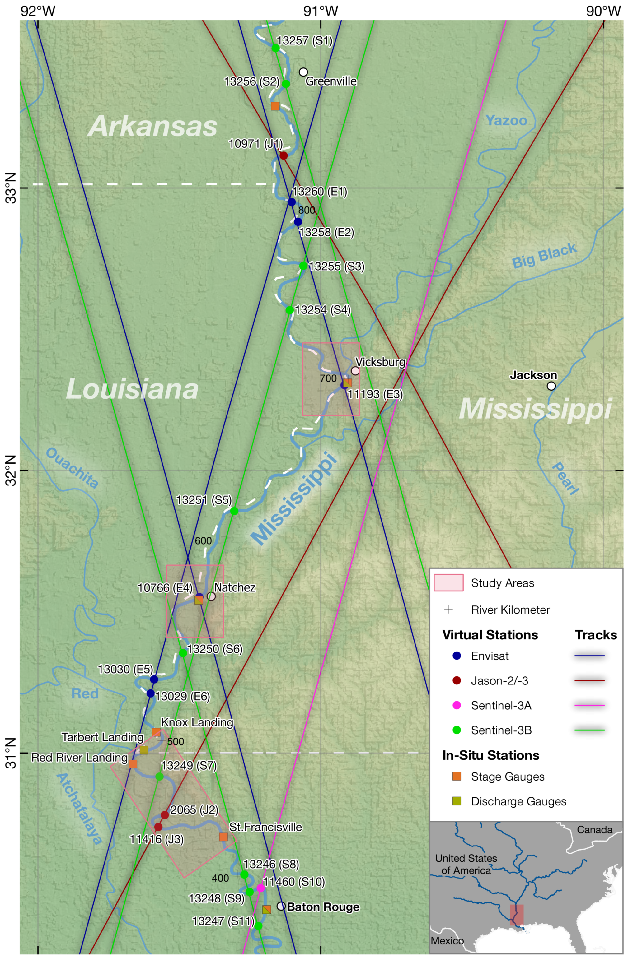
In this paper, we use only remote sensing data without calibration, because we are aiming to develop a method applicable to ungauged regions. However, a large variety of in situ data is required for the validation. Therefore, we chose the well surveyed Lower Mississipi River as study area. In contrast to existing similar AHG and also reach averaging approaches, we use significantly more remote sensing and satellite altimetry data. In addition to satellite altimetry, the Database for Hydrological Time Series over Inland Waters (DAHITI) [
21] provides long-term land-water masks and surface area time series since 1982 using satellite imagery from Landsat and Sentinel-2. Observational data gaps in these satellite images caused by clouds or sensor errors are filled using a long-term water occurrence mask allowing us to use every available satellite image [
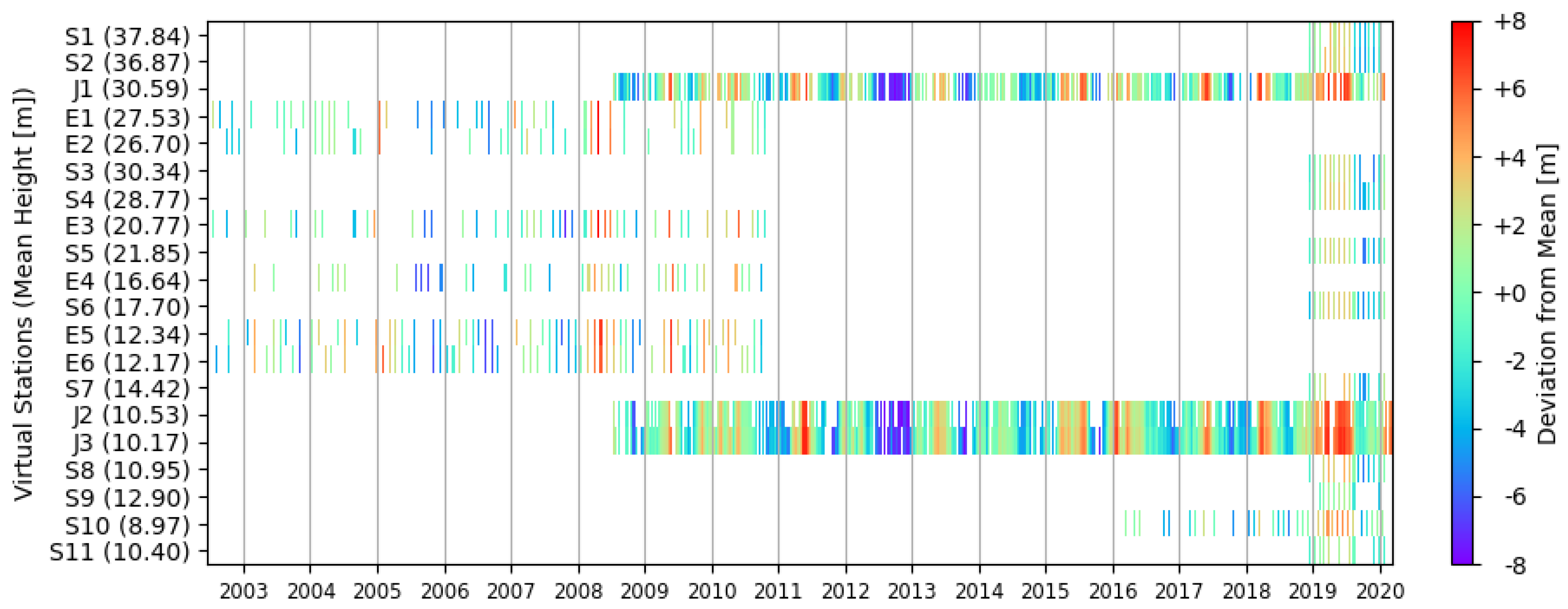
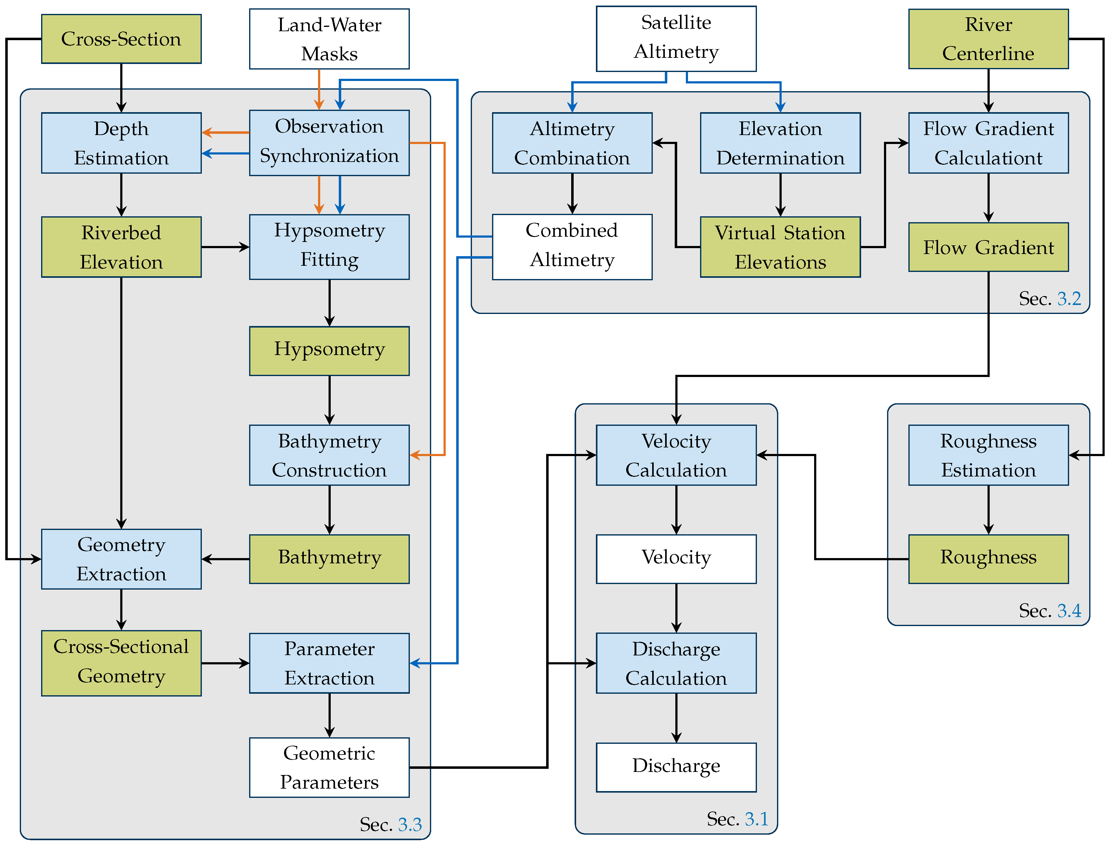
12]. To obtain a long-term water level time series from satellite altimetry observations available in DAHITI, we combine multiple virtual stations of the Envisat, Jason-2/-3, and Sentinel-3A/-3B missions covering different observation periods. We further increase the temporal coverage of available data by fitting a hypsometric function to synchronized satellite altimetry and surface area observations. Using the resulting hypsometry, we can predict the water level for each surface area observation derived from the images of the Landsat mission, which launched more than 20 years before the first satellite altimetry measurements over inland waters. The long-term satellite altimetry and remote sensing data allows us to construct large parts of the river bathymetry using observed instead of estimated data, because there are multiple occurrences of low water levels. Based on the predicted geometry, the velocity is estimated with the Manning Formula. The required roughness coefficient is estimated similar to other studies using adjustment factors [
38,
43,
47]. The flow gradient is derived from satellite altimetry measurements at multiple stations along the river. The resulting discharge time series are validated using in situ data. In situ measurements are substituted for the estimated parameters in order to analyze each parameter’s error and its effect on the residuals in the resulting discharge time series.
The article is structured as follows. In
Section 2 we introduce the selected study areas and describe the data used for processing and validation. In
Section 3 the methodology for estimating river discharge from remote sensing data is explained. In
Section 4 the results are presented and validated for each study area. The paper concludes with a discussion of the results in
Section 5 and a conclusion (
Section 6).
5. Discussion
This study is the first application of the DAHITI land-water and water occurrence masks on rivers. These masks and the modified hypsometric function were previously only used to determine the surface area, extent, and volume of lakes and reservoirs [
12,
26]. The study shows that also for large alluvial rivers that are morphologically more dynamic than lakes or reservoirs, the water occurrence mask can be used to extract a large amount of void-free land-water masks to fill data gaps caused by clouds, cloud shadows, instrument errors or ice. Additionally, the modified hypsometric function can be used to derive the water level within a river reach based on the respective surface area. However, it cannot be concluded that the approach is applicable to smaller rivers whose size does not exceed a few image pixels, or braided rivers which are morphologically much more dynamic than the Mississippi.
We showed in
Section 4.1 that the elevation differences between virtual stations of multiple missions with different observation periods can be estimated accurately within river segments without flow disruptions such as the Lower Mississippi River. This can be seen from the low inaccuracies resulting from the linear adjustment shown in
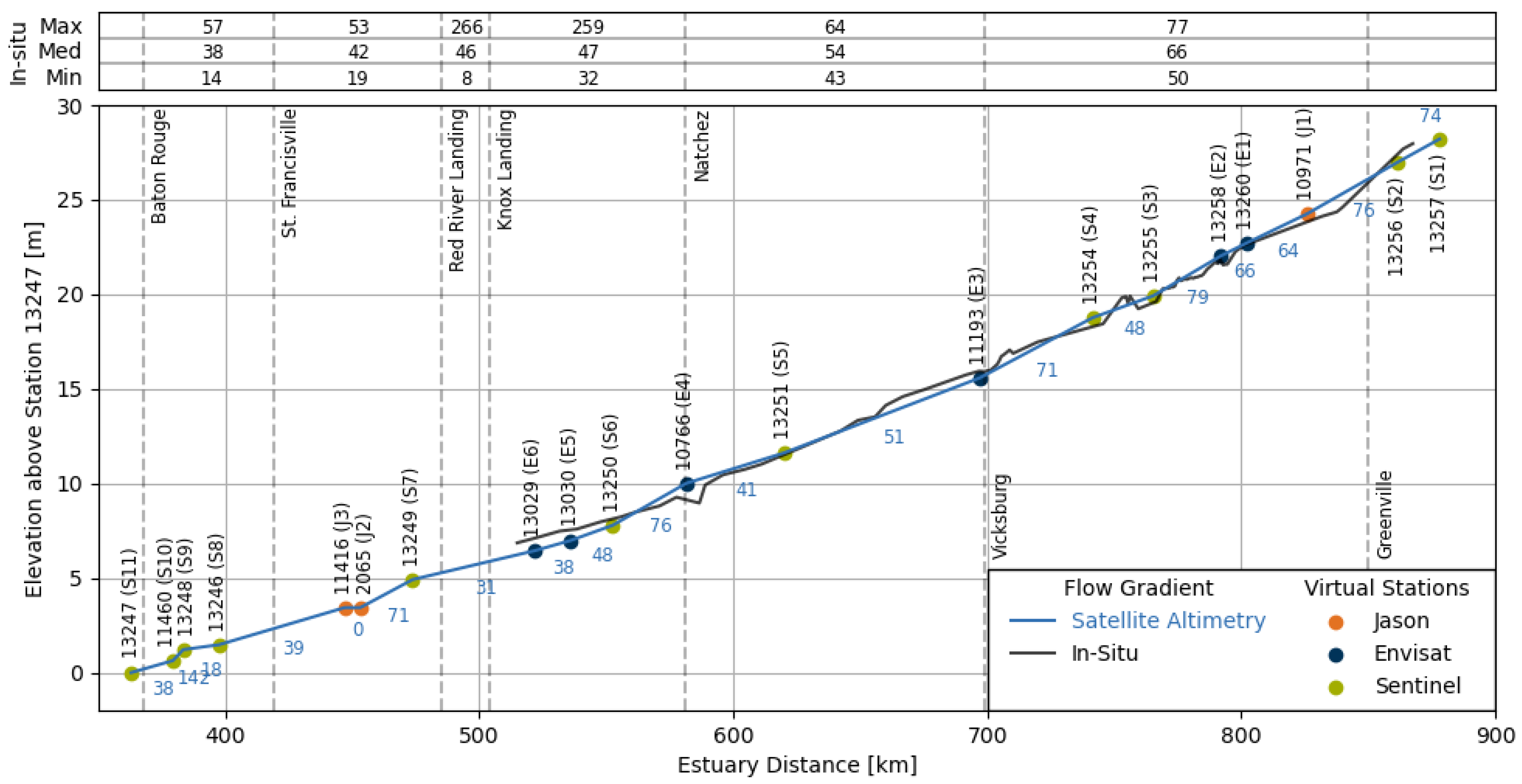
Table 2. Additionally, a comparison with the in situ values (
Figure 6) shows that the estimates are within the range of the variable in situ gradient and in general close to the median value. The largest deviations occur between adjacent stations. In contrast to the calculation of the flow gradient using SRTM or other DEM data which is limited to a short period of observation, the usage of multi-mission satellite altimetry allows the calculation of an average flow gradient over time. Using the mean values of each virtual station is not sufficient to calculate the flow gradient as these do not monotonically increasing with the estuary distance (see
Figure 2) which would result in a negative flow gradient. However, the continuity and variability of the flow gradient cannot be determined using our approach. The spatial resolution of the estimated flow gradient is limited by the fixed orbits of the satellite altimetry missions, but may be increased using long-repeat orbit missions such as Cryosat-2. In most cases a high spatial resolution of the flow gradient is of minor importance, but at Tarbert Landing (CS 492.5) a higher resolution would be beneficial to detect possibly rapid changes due to the upstream flow diversion. Deriving a variable flow gradient from a satellite-based sensor will first become possible with the SWOT mission.
The roughness coefficient is estimated using multiple adjustment factors, a method that has been well established in several studies [
38,
43,
47,
67]. Most of the adjustment factors are set to 0, because we select only uniform sections without irregularities such as eroded banks, abrupt changes in CS size, or obstructions based on the DAHITI water occurrence mask. However, the method is useful because different rates of meandering could be considered. There is no in situ data available for validation, but the calculated roughness coefficients are within the ranges of literature values for natural and maintained channels with solid bed materials which are common in alluvial rivers.
Our method differs from classical state of the art AHG approaches [
38,
41,
43] by the construction of the river bathymetry which uses as many observational data from satellite altimetry and remote sensing images as possible and a hypsometric function which was originally developed for lakes [
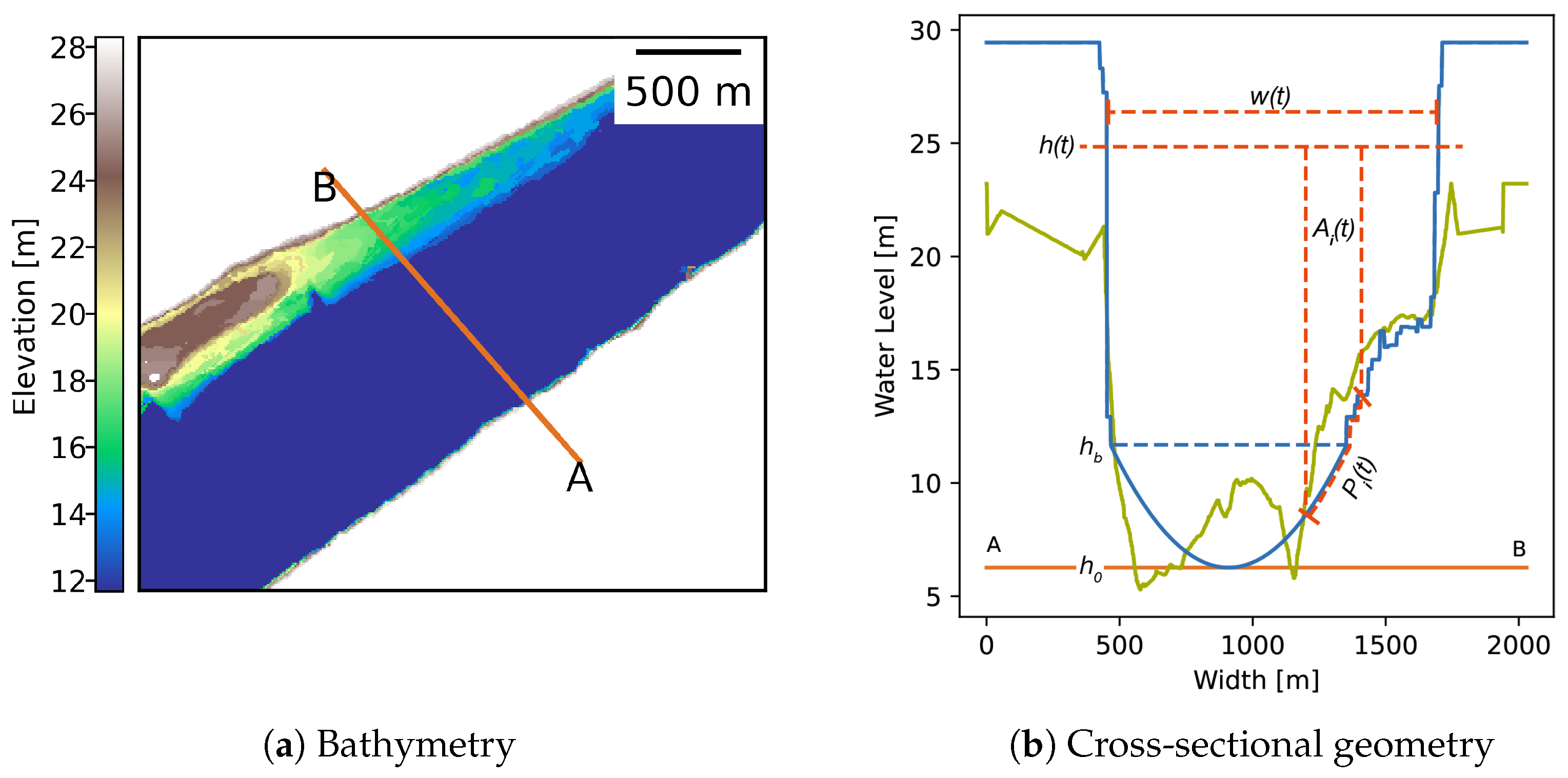
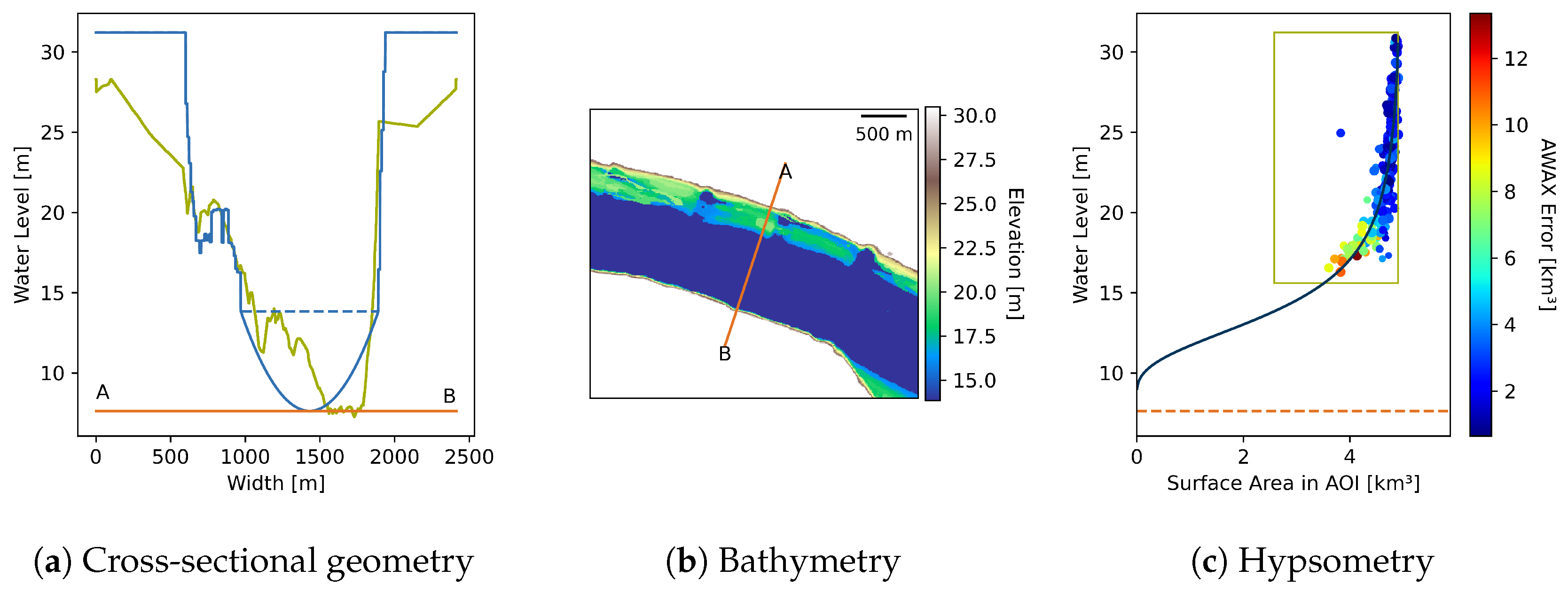
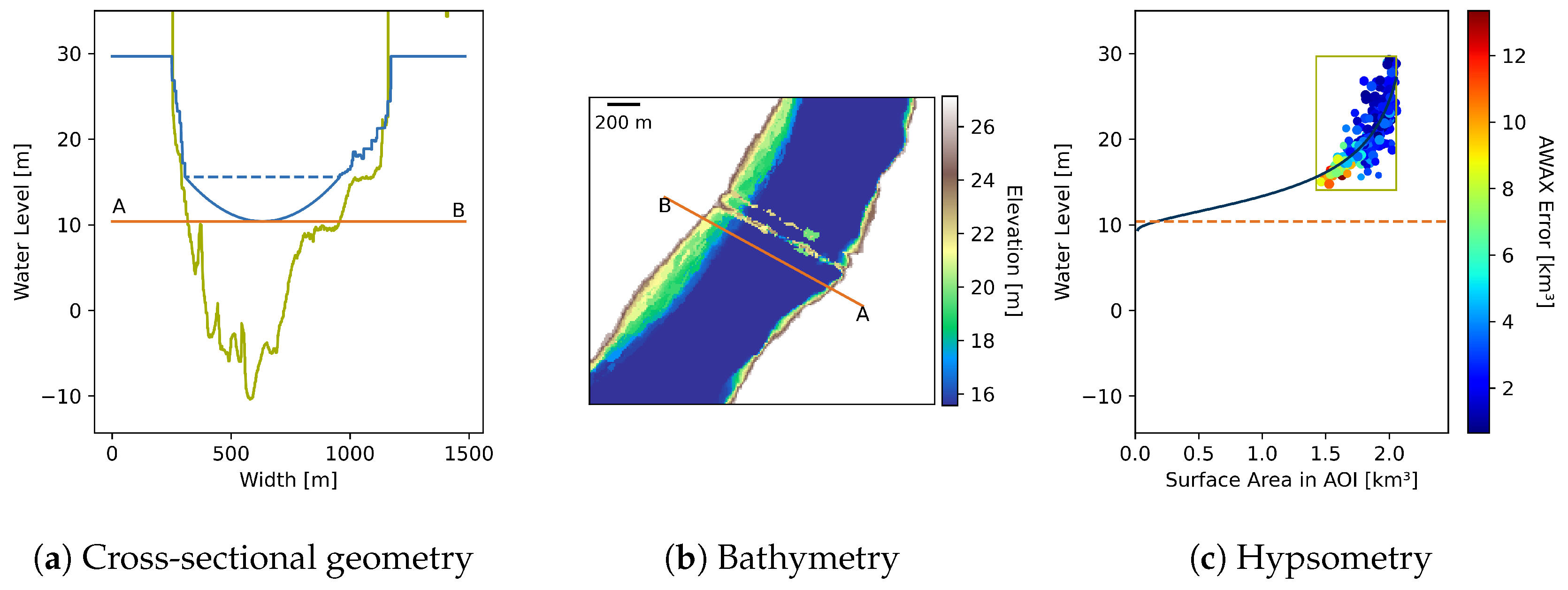
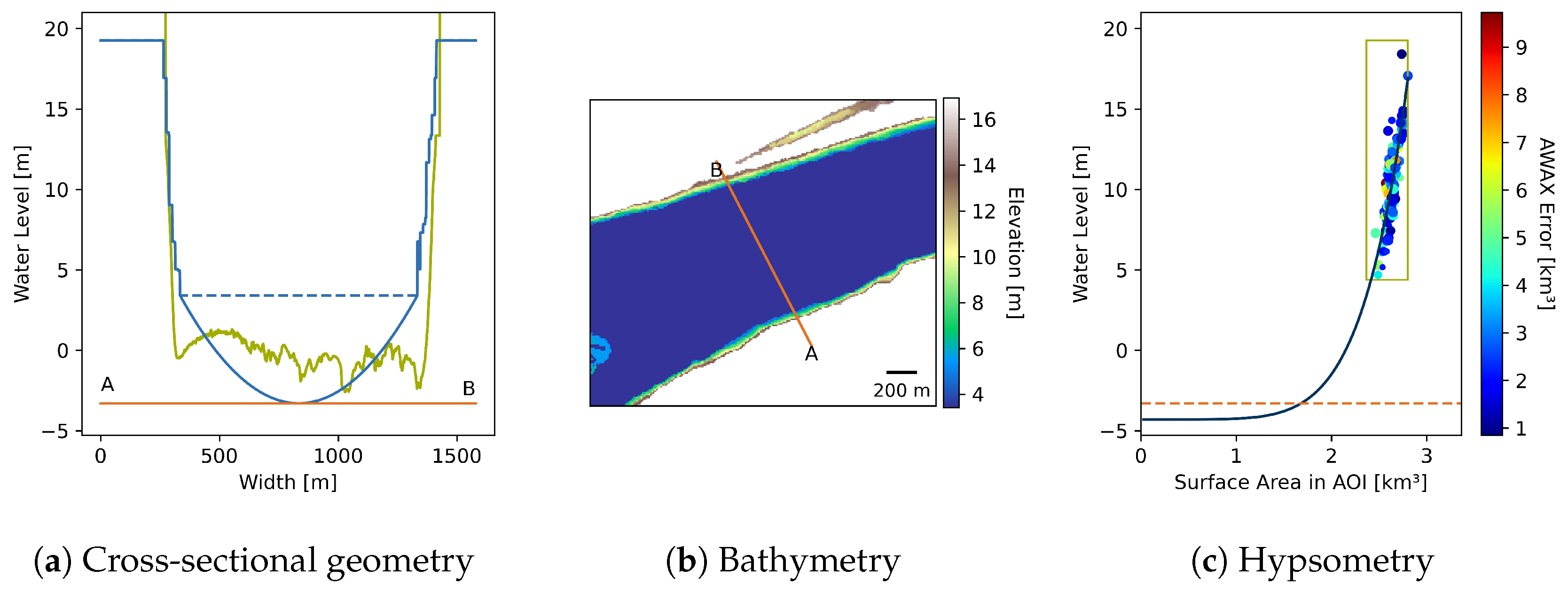
26]. Our results for 16 cross-sections show that the hypsometry can also be fitted to surface area and satellite altimetry observations over large alluvial rivers to increase the number of water level observations when the river depth is estimated correctly. The depth estimation succeeds for straight, wide, and uniform cross-sections with a median deviation of 2.4 m. We are able to manually identify such river segments using the DAHITI water occurrence mask. The method and its limitation to specific river segments might be transferable to similar rivers, because the empirical width-depth relationship used is derived from a large dataset of world-wide distributed rivers. The geometry extracted from the estimated bathymetry is validated using bathymetric survey data. Overall, the cross-sectional area is underestimated with an average coverage of 96.51% of the actual area. However, the average hydraulic radius is overestimated with 109.97% of the surveyed data, because of the medium spatial resolution of the Landsat mission and the parabola that is used to extend the geometry below the baseflow. The larger hydraulic radius leads to an increased velocity and thus discharge estimation, while the reduced area causes an underestimation of the discharge.
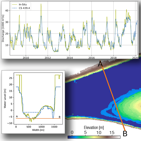
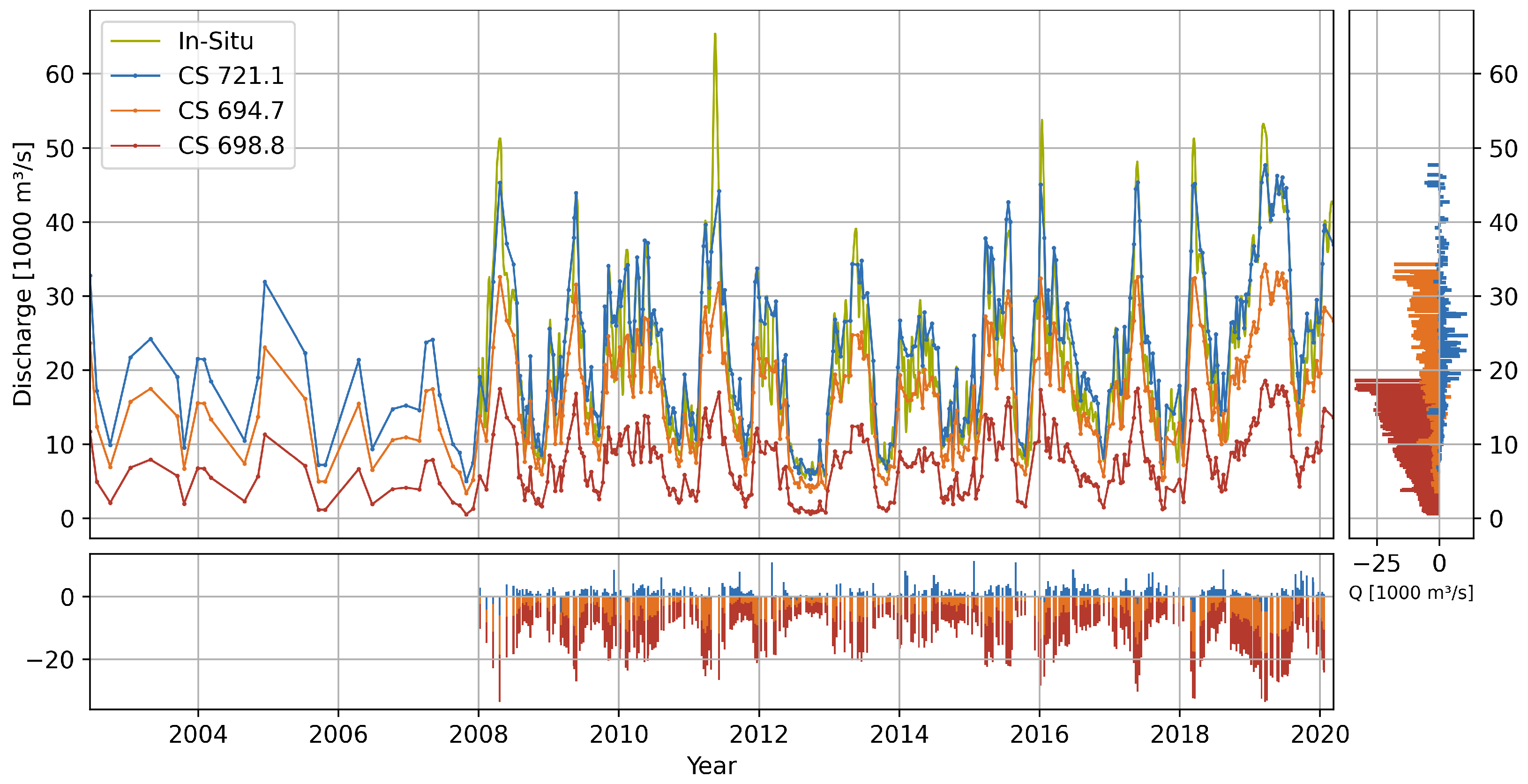
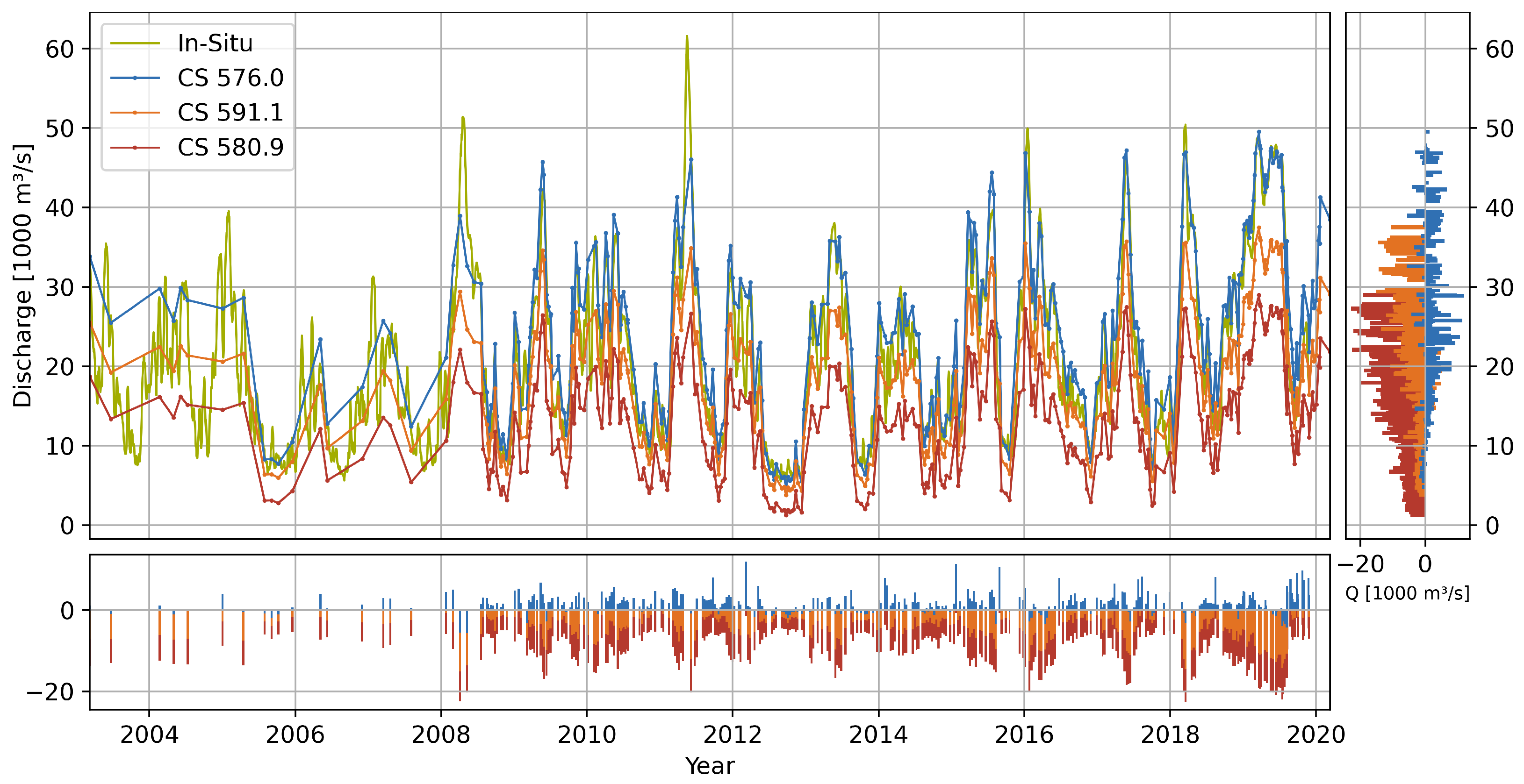
Using long-term satellite altimetry time series combined from multiple virtual stations enables the estimation of discharge time series over a period of up to 18 years. The validation at 16 cross-sections against the closest in situ measurements yields a median Normalized Root Mean Square Error (NRMSE) of 18.29% with a minimum of 10.95% and a maximum of 70.69%. The median Nash-Sutcliffe Efficiency (NSE) is 0.858 with a minimum of −1.112 and a maximum of 0.946. However, the resulting errors are significantly high at the three gauge locations. At Vicksburg and Natchez this is caused by the below average river width, which leads to an underestimation of the river depth and the depending geometric parameters. At Tarbert Landing the extracted channel geometry is correct, but the estimated flow gradient is most likely too low. At the 13 other cross-sections, which are not defined by the gauge locations but are selected to be in straight, wide, and uniform river segments, the median NRMSE is 13.26% with a minimum of 10.95% and a maximum of 28.43%. The median NSE at these cross-sections is 0.921 with a minimum of 0.658 and a maximum of 0.946. These errors are within the range of results from an intercomparison of state of the art studies [
44].
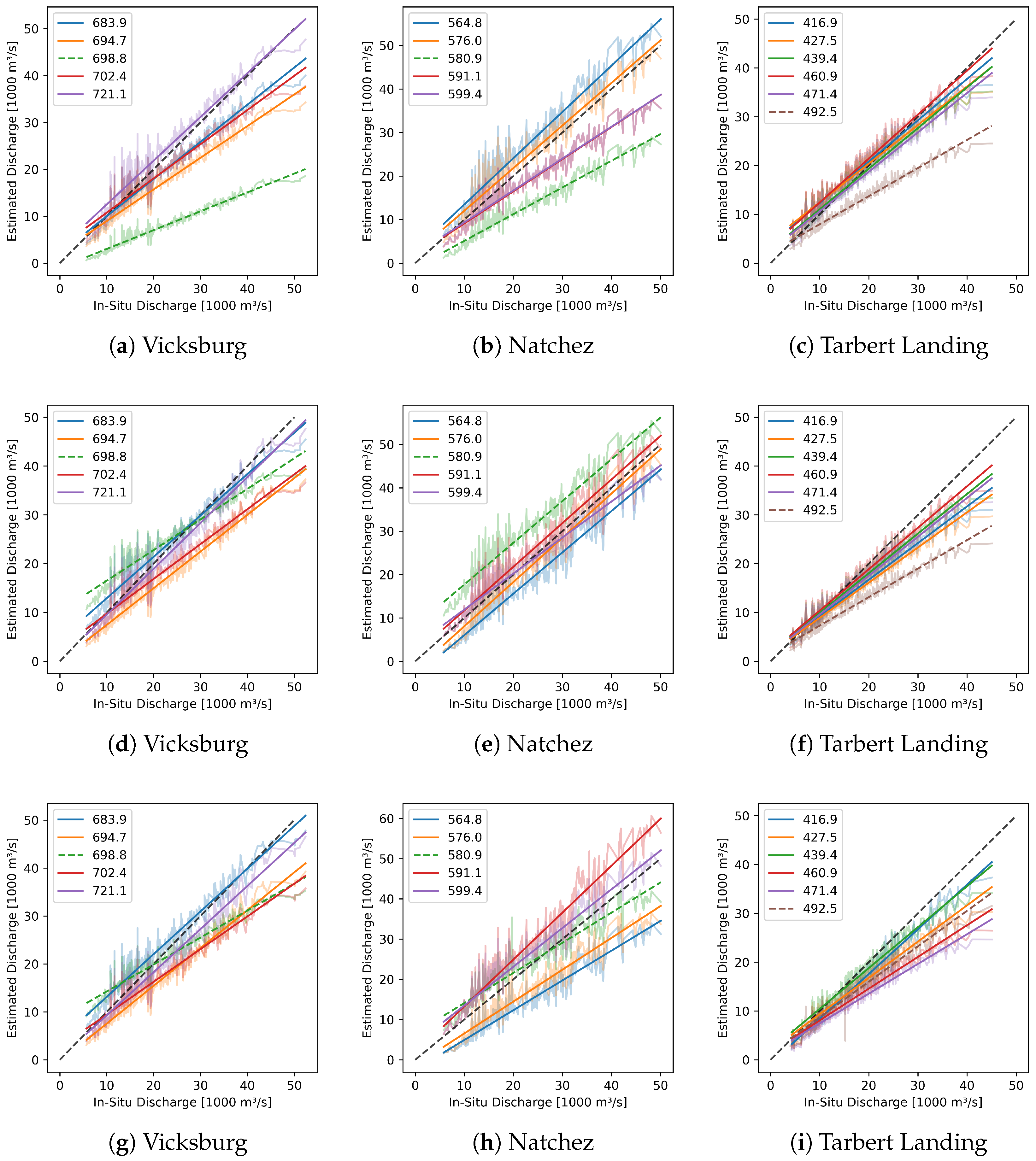
In contrast to the variable distribution of errors, the correlations between estimated and in situ discharge are consistently high at all cross-sections with values above 0.95.
Figure 14a–c show the linear regressions of estimated and in situ discharge for each CS. It is apparent that the discharge is predominantly underestimated at each CS and the deviation increases with rising discharge. At Tarbert Landing the results of the selected CS are very consistent, while they are more widely spread at Natchez and Vicksburg.
To evaluate the quality of the estimated geometric parameters, we substitute the estimated cross-sectional geometry with a geometry extracted from the bathymetric survey data and calculate an additional time series for each CS.
Figure 14d–f show the relation of these new estimates and the in situ discharge. The estimates improve for CS 698.8 at the Vicksburg gauge and CS 580.9 at the Natchez gauge which is expected as the geometry is clearly underestimated. This emphasizes the high importance of correctly estimated geometric parameters. However, the estimated discharge at CS 580.9 is now consistently too high. This could be caused by an overestimated flow gradient which is much smaller downstream at CS 576.0 and CS 564.8 where the estimated discharge decreased using the bathymetric survey data. At Tarbert Landing the estimates do not change significantly, which confirms that the geometric parameters are estimated well.
Next, we use the in situ flow gradient time-series derived from in situ water-level time series (see
Figure 6) to substitute the estimated constant slope. The variable flow gradient is used in two analyses. First,
Figure 14g–i show the relation of in situ discharge and estimates using bathymetric survey data and variable in situ flow gradient. In this analysis, all parameters are extracted from in situ data except the roughness which has to be estimated anyway and the input water level time series which is obtained from satellite altimetry. Compared to the results shown in
Figure 14d–f, the estimates improve e.g., at the Tarbert Landing (CS 492.5) and Natchez gauge (CS 580.9) where we expected the estimated gradient to be wrong. However, at some CS (e.g., CS 460.9) there is a higher discharge deviation using the variable gradient and bathymetric survey data. Therefore, we assume that the estimated roughness must be wrong at those places. In the second analysis, we use the estimated bathymetry and the variable in situ flow gradient.
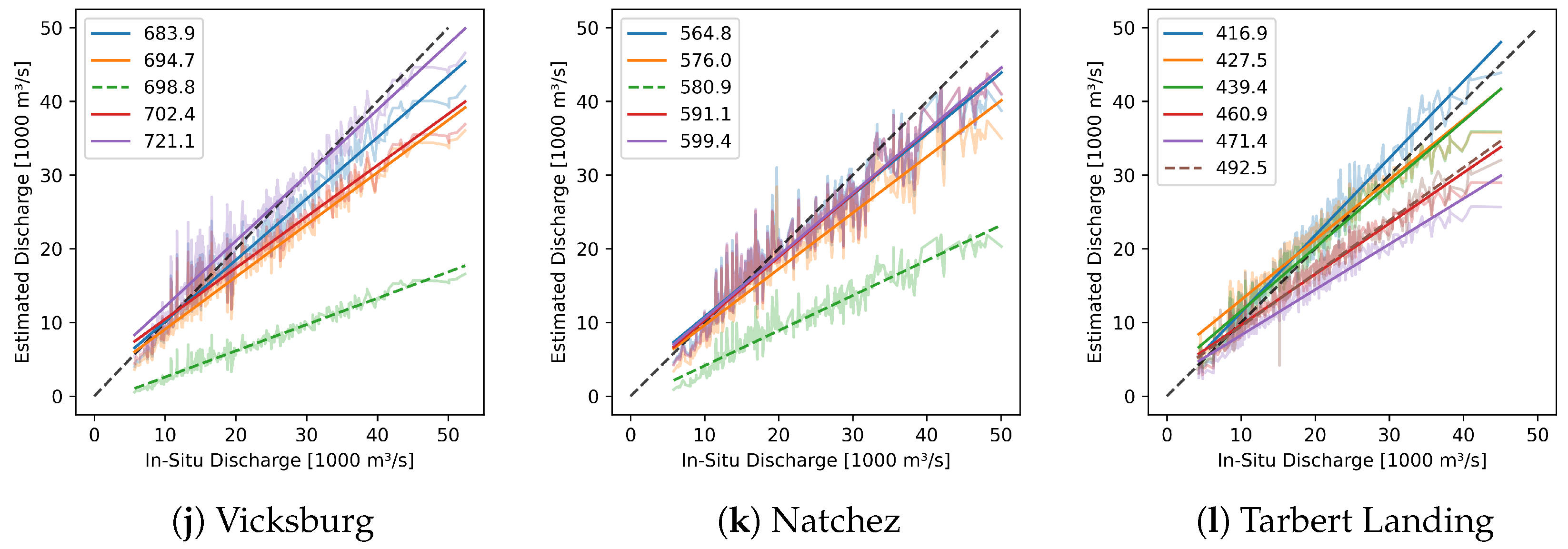
Figure 14j–l show the respective relation of in situ data and estimates. Again, the results are worst at the narrow CS 698.8 and 580.9 where the estimated bathymetry is too shallow. The use of the variable flow gradient shows no improvement in the results of these CS compared to
Figure 14a–c. At Natchez, the results get more consistent at the different CS while they are more widely spread at Tarbert Landing using the variable flow gradient.
Table 6 shows the NRMSE values per CS for each substitute and additionally the assumed significant factor for further improvements of the methodology which is chosen as follows: If the NRMSE increases or the improvements are only marginal using substituted values of
I,
A and
P, we assume the roughness to be significant for further improvements. If the NRMSE decreases significantly by either substituting
I or
A and
P we assume the respective substitute to be significant for further improvements but only when the effect is not negated using all substitutes.
At CS 721.1, 702.4, 683.9, 591.1, 576.0, 564.8, 471.4, 460.9, 427.5, and 416.9 single or no substituted parameters lead to improvements while the errors increase when all parameters are substituted. As we expect the results to improve using the substituted parameters, the estimated roughness must be the cause of error. At CS 694.7 and 439.4 the estimation improves using the substitutes but the remaining error is still high compared to the improvements. Therefore, the roughness must also be the significant parameter at these locations to gain further improvements. At CS 698.8 and 580.9 the results significantly improve by substituting the geometric parameters. These are predominantly the narrow CS at the gauges where the bathymetry construction failed caused by the underestimation of the river depth. At CS 599.4 the substitution leads to significant improvements but the remaining errors are still high. Therefore, all parameters (I, A, P, and the roughness) are significant for improvements. CS 492.5 is the only location where the result improve significantly using the in situ flow gradient and the effect was not dampened by substituting the bathymetry. Here, the estimated flow gradient is probably incorrect due to the flow diversion just upstream of Tarbert Landing.
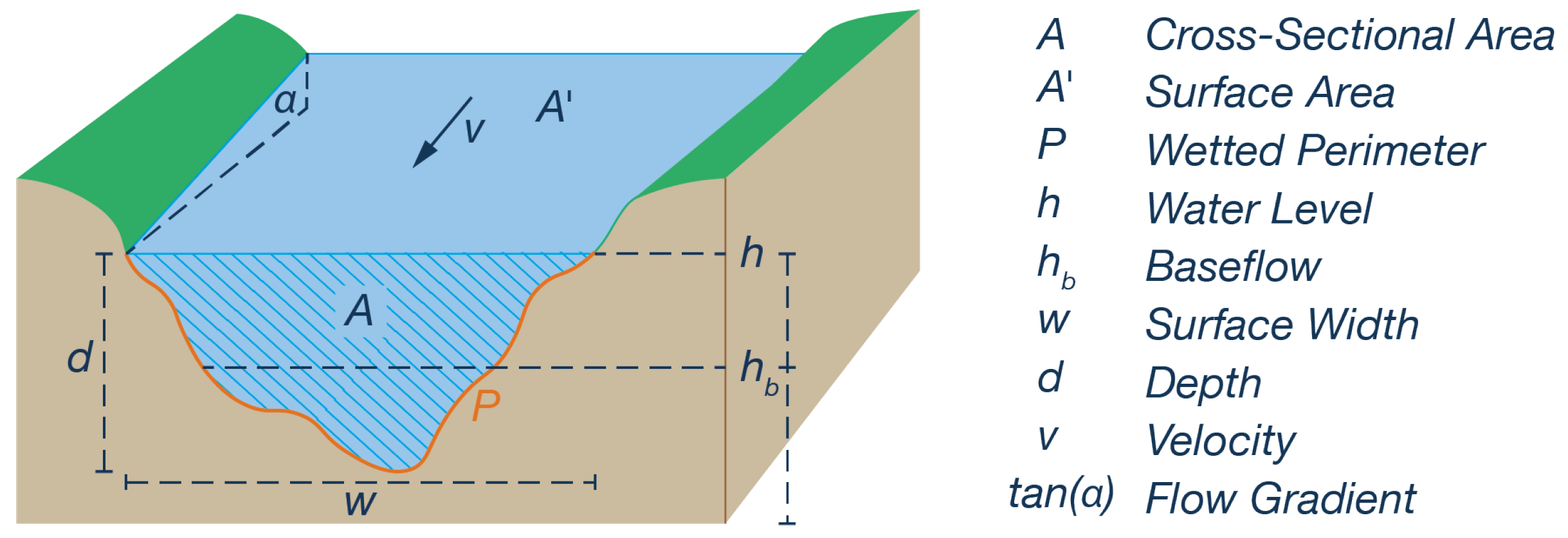
Although the number of 16 CS as test locations might be too low to be statistically significant and the CS are manually selected, the substitution of parameters shows that the largest cause of error is the incorrect roughness value. This is probably not only caused by the coarse estimation of the roughness coefficient using adjustment factors but also by the used flow formula itself. To estimate the flow velocity we use the Manning formula which is the most commonly used relation between velocity and water level described by a friction factor. However, being an empirical equation, the Manning formula has no theoretical basis. It is inhomogeneous in terms of dimensional analysis and the value of the roughness coefficient has no direct relation on the properties that cause bed roughness. Furthermore, using the Manning formula we can only obtain an average velocity over width and depth, and complex characteristics as backwater effects, negative flow gradients or uneven velocity distributions due to meandering cannot be considered. We minimize the effect of generalization in width by dividing the CS in multiple subsections but to overcome the velocity distribution over depth and the other mentioned challenges a more sophisticated formula will be required. Some improvements can be expected by using a variable roughness coefficient as it is the standard for non-remote sensing methods and already used by Bjerklie et al. [
41] with remote sensing data.
6. Conclusions and Outlook
In this paper, we present an approach to determine long-term river discharge time series using solely satellite altimetry and remote sensing data at the Lower Mississippi River. The methodology does not require calibration and works at cross-sections in straight, wide, and uniform reaches of the river and possibly at comperable large alluvial rivers. At river segments without flow disruptions, a linear adjustment of the virtual station elevations allows us to combine satellite altimetry data from multiple virtual stations and missions to one single long-term water level time series. At the Lower Mississippi River, the constant flow gradient derived from the virtual station elevations shows a high agreement with the average of the variable flow gradient calculated using in situ data. The roughness coefficient is estimated using multiple adjustment factors similar to many state of the art studies. Using long-term optical remote sensing data and a hypsometric function, further water levels can be derived from surface areas in addition to the satellite altimetry observations. In this way, we can cover a wider range of water levels and use it in combination with the respective water surface extents to construct large parts of the river bathymetry. The remaining part of the bathymetry below the baseflow is approximated using a parabola and an estimation of the river bed elevation which is based on an empirical width-to-depth relationship that shows limitations in below average wide cross-sections.
In straight, wide, and uniform river reaches, the NRMSE varies between 10.95% and 28.43% and is comparable with other studies without calibration. The NSE is in a range from 0.658 to 0.946. The NRMSE increases up to 70.69% at CS not defined by the planform shape of the river but by gauges which are predominantly located in narrow reaches where depth is underestimated in our approach.
To discuss the significance of the parameters in the Manning formula, we substitute in situ measurements of bathymetry and variable flow gradient for the respective estimated parameters. Except for narrow CS where the in situ bathymetry leads to the smallest residuals, overall roughness is the most significant parameter for further improvements of the methodology. The in situ flow gradient was only significant at one CS of the study where the spatial resolution of the satellite altimetry was too low to detect a larger change of the flow gradient.
The case study at the Lower Mississippi river shows that the approach is limited to selected regular and uniform reaches where the flow is not disturbed by obstacles, bends, or abrupt changes in width. Such conditions cause an underestimation of the channel depth using the empirical width-depth relationship. However, potentially suitable reaches can be identified based on the DAHITI water occurrence mask. At CS in these reaches, the geometry can be approximated well, because of the large number of synchronized water level and surface area observations and the derived hypsometry. Since the estimated flow gradient matches the mean of the variable in situ data, only the difficult to determine roughness coefficient remains as a limiting factor for the application of the methodology in suitable reaches.
For future studies, improvements of the roughness estimation and selection of cross-sections will be a particular challenge. In particular, the applicability and potential of more sophisticated flow equations should be examined. Additionally, the transferability to other targets such as smaller, braided, or non-alluvial rivers should be studied. The principle of mass conservation and reach averaging could be used to reduce the currently wide range of errors. Using water levels derived from surface areas with a hypsometry [
26] would extend the resulting discharge time series over the period of the Landsat mission starting with the launch of Landsat 4 in 1982. The implementation of additional remote sensing missions gives new possibilities. Cryosat-2 data could be used to increase the spatial resolution of the estimated flow gradient and in future, the time synchronous observations of water level, surface area, and time variable flow gradient by the SWOT mission could be used to improve all aspects of our methodology while the effort of an implementation of SWOT data should be small.


