Article

Direction-of-Departure and Direction-of-Arrival Estimation Algorithm Based on Compressive Sensing: Data Fitting

1
Department of Information and Communication Engineering, Sejong University, Seoul 05006, Korea
2
Department of Defense Systems Engineering, Sejong University, Seoul 05006, Korea
*
Author to whom correspondence should be addressed.
Remote Sens. 2020, 12(17), 2773; https://doi.org/10.3390/rs12172773
Submission received: 17 July 2020 / Revised: 21 August 2020 / Accepted: 24 August 2020 / Published: 26 August 2020
(This article belongs to the Section Remote Sensing Image Processing)

Abstract

:
In this paper, a compressive sensing-based data fitting direction-of-departure/direction-of-arrival (DOD/DOA) estimation algorithm is proposed to apply the superior performance of compressive sensing method to the bistatic MIMO sonar systems. The algorithm proposed in this paper optimizes the output data via convex optimization-based sparse recovery, so that it is possible to estimate the DOD and the DOA for each target accurately. In order to minimize the amount of computation, the cost function with constraint condition is implemented in this paper. Furthermore, the constraint condition parameter of the cost function is analytically derived. Through various simulations, it is shown that the superior DOD and DOA estimation performance of the proposed algorithm and that the analytical derivation of the constraint condition parameter is useful for determination of regularization parameter.

1. Introduction

Conventional direction-of-arrival (DOA) estimation algorithms estimate the DOA of the signal source using the phase difference between the elements constituting the sensor array. Examples of such algorithms are conventional beamforming, adaptive beamforming, and MUSIC (Multiple Signal Classification) [1,2,3]. Methods of estimating DOA in a different way from the conventional method have been proposed [4,5,6,7,8,9,10,11,12,13]. The schemes are based on compressive sensing.
The compressive sensing CS-based DOA estimation method is a technique for estimating DOAs by using the sparse property of a signal when incident signals are spatially sparse. Figure 1 shows the concept of the CS-based DOA estimation method.
The received signals used for DOA estimation methods are incident on the sensor array at specific angles. Therefore, the received signals can be said to be spatially sparse as the signals are only incident in specific angles, not in all the angles.
In [4], a method of extending single measurement or multiple measurements to beam space and performing sparse recovery using basis pursuit denoising (BPDN) has been presented. Furthermore, in order to solve the computational problem that occurs when using multiple measurements, a L1-SVD method that performs sparse recovery using singular vectors of multiple measurements has been proposed.
The convex optimization based sparse recovery used in [4] requires a large amount of computation. In [5], to decrease the computation of the sparse recovery, a method of approximating the l 0 norm minimization problem, which is a discontinuous problem, with a continuous function and performing sparse recovery using a gradient descent method has been presented.
In [6,7,8], compressive sensing-based covariance fitting methods have been studied. In [9], a compressive sensing-based covariance fitting algorithm using iterative operation sparse iterative covariance-based estimation (SPICE) has been presented. As SPICE does not perform sparse recovery using BPDN, it requires less computation that the existing covariance fitting algorithms [6,7,8].
In [10], a sparse spectrum fitting (SpSF) DOA estimation algorithm is introduced and its effective regularization has been studied. A weight used in the cost function of SpSF depends on the number of snapshots. In [11], an optimal weight of the cost function setting method according to the number of snapshots has been presented.
The phase error of the uniform linear sensor array has a great effect on the estimation performance of the DOA estimation algorithms. In [12], a new compressive sensing-based DOA estimation algorithm that repeatedly estimates the phase error and DOA has been proposed.
The conventional compressive sensing-based DOA estimation methods depend on the noise field. In [13], to make it possible to estimate DOA based on the compressive sensing method even in the unknown noise field, a new compressive sensing-based DOA estimation algorithm based on the generalized correlation decomposition algorithm has been presented.
The CS-based DOA estimation method is utilized for estimating DOAs by spectralizing the signal data vector itself using the property that the received signal is spatially sparse. In addition, the CS-based DOA estimation method estimates DOAs by optimizing a sparse output signal data with two constraints of sparsity reduction and sensor data model fitting. Therefore, the CS-based DOA estimation is more robust to sensor elements failure in comparison with the non-CS-based DOA algorithm. In addition, the performance of the CS-based DOA estimation algorithm does not degrade significantly with the decrease of sensor elements spacing and the decrease of the number of sensor elements in comparison with non-CS-based algorithms.
Target strength (TS) technology is currently being developed to avoid detection of the passive sonar system. Geometric modeling to minimize the target strength has been applied to the submarines and vessels. This technique significantly degrades the performance of the existing DOA estimation algorithms.
The bistatic multiple input multiple output (MIMO) sonar system is the solution to the problem of detecting the low TS submarines or vessels. This is a system in which two sensor arrays are divided and performed by a transmitter and a receiver, rather than performing both transmission and reception in a sensor array. When using the bistatic MIMO sonar system, the receiver estimates the direction-of-departure (DOD) and the DOA. The two sensor arrays can change roles and can detect a low TS target of the stealth technology by estimating the DOD and DOA.
In order to detect the low TS submarines or vessels, a number of DOA estimation algorithms implemented in bistatic MIMO sonar systems have been extensively studied. The conventional beamforming, the adaptive beamforming and MUSIC, which are representative DOA estimation algorithms, have been expanded to the DOD/DOA estimation algorithms [14,15,16,17,18,19].
In [14], a DOD/DOA estimation method has been proposed by applying ESPRIT to the bistatic MIMO radar system. In [15,16], MUSIC has been applied to the bistatic MIMO system and a method to estimate DOD and DOA separately has been proposed.
In [17], a joint DOD/DOA estimation method using ESPRIT and SVD of an array covariance matrix form transmit subarrays has been presented. The proposed scheme in [17] can estimate the DODs and DOAs of targets in closed-form and pair automatically.
In [18], the bistatic co-prime multiple input and multiple output arrays have been considered to estimate multiple far-field targets. Using the scheme presented in [18], many DOA estimation methods for ULA can be applied to the sparse bistatic MIMO array and with closed-form degree of freedom (DOF) presented in [18]; it can have an advantage in terms of array aperture.
In [19], to estimate the DOD and DOA and the Doppler shift of a moving target for a MIMO radar system, a reduced dimension and low complexity algorithm has been proposed.
In order to take advantage of the superior performance of the DOA estimation based on compressive sensing in the bistatic MIMO sonar system, this paper proposes a compressive sensing-based DOD/DOA estimation algorithm in the bistatic MIMO sonar system.
Among the compressive sensing-based algorithms, it is shown that the DOD/DOA estimation is possible in the case of orthogonal matching pursuit (OMP), which is a greedy algorithm [20]. However, in the case of greedy algorithms, there is a condition that the received signal is spare. That is, the number of targets must be known in advance. The proposed algorithm in this paper optimizes the output data as sparse by searching the solution through convex optimization, so that it is possible to estimate the DOD and the DOA for each target accurately. It has been shown that CS-based DOA estimation algorithms are superior to non-CS-based DOA estimation algorithms at the expense of much computational burden. In this paper, it is shown how the CS-based DOD/DOA estimation algorithm outperforms non-CS-based DOD/DOA estimation algorithms. The reduced-dimension cost functions based on fast Fourier transform (FFT) for moving targets was derived.

2. Signal Modeling of Bistatic MIMO Sonar System

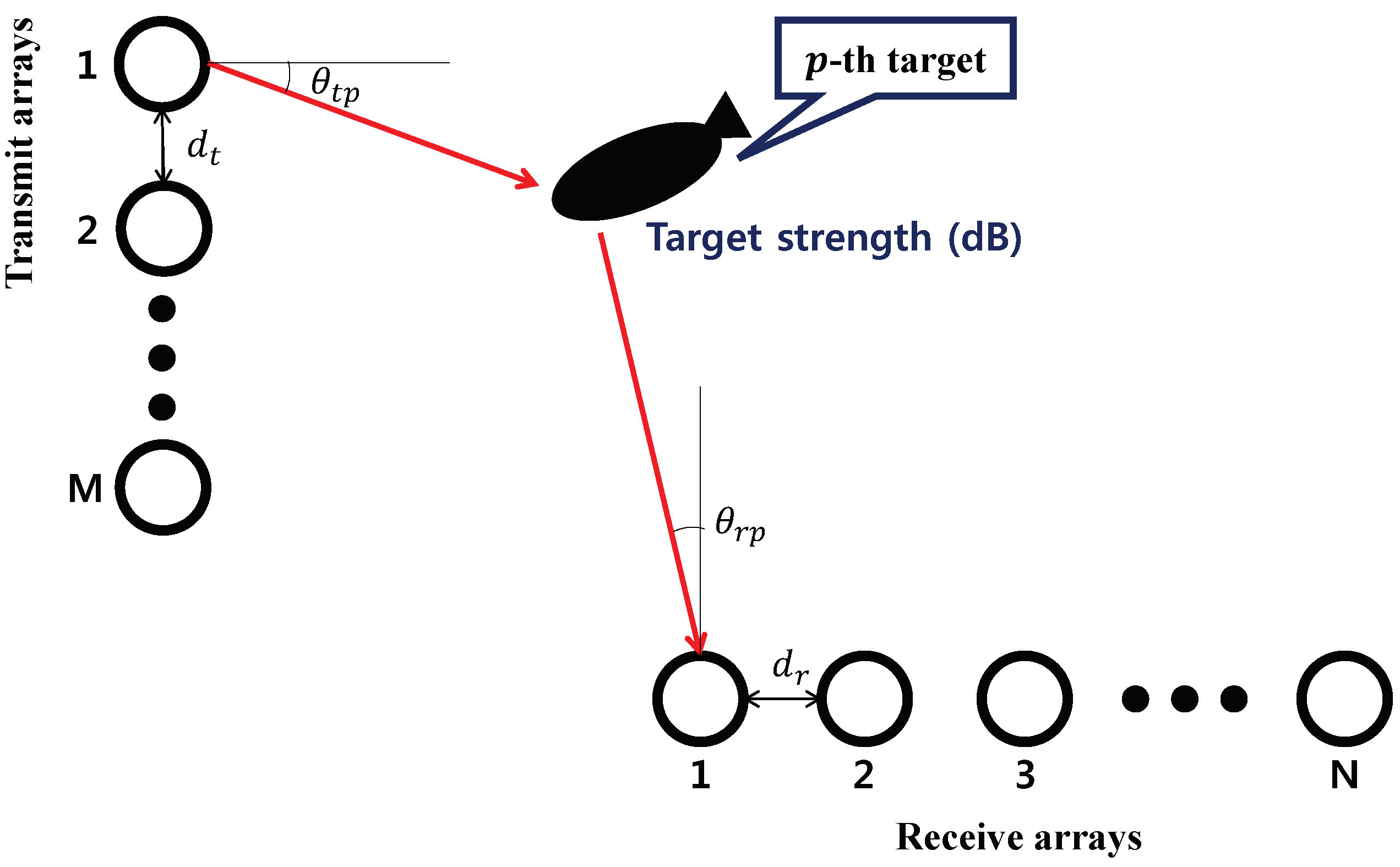
In this section, the bistatic MIMO sonar signal model [14] used in this paper is presented. The transmit and receive arrays are uniform linear array (ULA). The transmitter array has M elements and receiver array has N elements. λ denotes the wavelength. Let d t and d r be the inter-element spacing at the receiver and transmitter, respectively. The number of targets is P. Assume that the DOD and the DOA for the p-th target be expressed as θ t p and θ r p , respectively. The array vector for the n-th sensor of receiver can be written as
a n θ r p = exp j 2 π λ n 1 d r sin θ r p .
The array vector for the m-th sensor of transmitter can be written as
b m θ t p = exp j 2 π λ m 1 d t sin θ t p .
Using (1), the receiver steering matrix A r can be written as
A r = a 1 θ r 1 a 1 θ r P a N θ r 1 a N θ r P .
Using (2), the transmitter steering matrix A t can be written as
A t = b 1 θ t 1 b 1 θ t P b M θ t 1 b M θ t P .
In the case of P targets, α ¯ is defined as
α ¯ = α 1 , , α P T
where α 1 , , α P are the target strengths of each target.
A coded pulse of the transmitter can be expressed as a matrix S :
S = s 1 s 2 s M T s i = s i t 1 s i t 2 s i t L s j = s j t 1 s j t 2 s j t L , i j , i , j = 1 , , M
where s i is the transmitted signal from i-th sensor of the transmitter and s j is the transmitted signal from j-th sensor of the transmitter. These vectors are designed as orthogonal to each other to distinguish signals of each of the transmitters after matched filtering. The number of snapshots is L:
N = n 1 1 n 1 L n N 1 n N L .
where N is the matrix of noise. The noise is complex-valued and the real part and the imaginary part of the noise are independent Gaussian random variables with zero mean. The variance of the real part is denoted by σ 2 / 2 , which is equal to the variance of the imaginary part, σ 2 / 2 .
The received signal matrix can be written as
X = A r · diag α ¯ · A t T · S + N .
After matched filtering the signal, the output of the filter can be expressed as
Y = 1 L X · S H .
By transforming the matched filtered signal to an independent sufficient statistic vector, the signal data becomes applicable to the DOD/DOA estimation methods. In case the number of targets is one, the independent sufficient statistic vector can be expressed as
η = row Y = row 1 L n = 1 L X n S n H = row 1 L n = 1 L α a θ r b θ t T S n S n H + N n S n H = row α a θ r b θ t T n = 1 L 1 L S n S n H + 1 L n = 1 1 N n S n H = row α a θ r b θ t T R s + row 1 L n = 1 1 N n S n H = α k θ r , θ t + v .
The signal covariance matrix R s can be written as
R s = n = 1 L 1 L S n S n H .
The array vector reflecting the bistatic MIMO sonar system can be expressed as
k θ r , θ t = row a θ r b θ t T R s .
row(·) denotes the operator that stacks the rows of a matrix in a column vector. The noise vector passed through the matched filter can be written as
v = row 1 L n = 1 1 N n S n H .
When the number of targets is P (more than two), the array manifold of the bistatic MIMO sonar system can be written as
K θ t , θ r = k θ t 1 , θ r 1 , , k θ t P , θ r P , k θ t , θ r = a 1 θ r b 1 θ t a 1 θ r b 2 θ t a 1 θ r b M θ t a 2 θ r b 1 θ t a N θ r b M θ t .
When Q transmit pulses are used, the target strengths matrix H can be expressed as
h q = α 1 ( q ) α 2 ( q ) α P ( q ) T , q = 1 , , Q H = h 1 h 2 h Q H = α 1 ( 1 ) α 1 ( 2 ) α 1 ( Q ) α 2 ( 1 ) α 2 ( 2 ) α 2 ( Q ) α P ( 1 ) α P ( 2 ) α P ( Q ) .
In this case, the matrix of the noise can be written as
V = v 1 , v 2 , v Q .
Only stationary targets are considered in this paper. Therefore the target strengths are constant in a pulse, and the target strengths are independent from pulse to pulse, rather than scan to scan.
When the number of targets is P (more than two) and multiple transmit pulses are used, the independent sufficient statistic matrix Y η can be expressed as
Y η = K θ t , θ r H + V .
When a single transmit pulse is used, the independent sufficient statistic vector y η can be expressed as
y η = K θ t , θ r h + v .

3. Bistatic Data Fitting DOD/DOA Estimation Algorithm

As in (18), in case of using one pulse, the signal data used for the DOD/DOA estimation can be obtained in the form of a vector in bistatic MIMO sonar system even if the transmitter sent a coded pulse into multiple snapshots. When only one pulse is used, the cost functions of the compressive sensing-based data fitting DOD/DOA estimation algorithm in bistatic MIMO sonar system can be obtained by applying the compressive sensing-based data fitting DOA estimation algorithm using a single snapshot [4].
The cost function of compressive sensing-based data fitting DOD/DOA estimation algorithm for determination of h without restrict condition can be defined as
h = arg min h y η K h 2 2 w h 1 .
In the case of (19), the weight parameter w controls the trade-off between the sparsity of the estimated data h 1 and the difference between y η and K h according to a given value.
By repeating the optimization process through the cost function of (19), we find the sparse signal covariance vector among countless solutions.
In the case of (19), as the convex optimization needs to be performed many times while changing the weight value w, it requires a large amount of operation time.
The cost function of compressive sensing-based data fitting DOD/DOA estimation algorithm for determination of h with constraint condition can be defined as
min h h 1 s . t . y η K h 2 2 β 2 .
Minimizing the number of non - zero elements of the signal vector s . t . Independent sufficient vector Arraymanifold · Signal vector 2 2 Parameter of the constraint condition
In the case of (20), it is possible to obtain a sparse output value through a single optimization. To use this algorithm, the parameter of the constraint condition β 2 needs to be determined.
In [4], the parameter of the constraint condition of the compressive sensing-based data fitting DOA estimation algorithm has been derived by using the fact that the real part and the imaginary part of the noise are independent Gaussian random variable with zero mean.
On the other hand, in the case of the bistatic MIMO sonar system, as the matched filter is used, the characteristic of the complex Gaussian noise can not be utilized as in [4].
To achieve the parameter of the constraint condition β 2 of (20), the mean of v 2 2 and standard deviation of v 2 2 are used in this paper.
The parameter of the constraint condition β 2 can be written as
β 2 = E v 2 2 + 6 · std v 2 2 .
In the case of the constraint condition parameter β 2 , it should be able to accommodate most random variables of v 2 2 . Usually, the mean of v 2 2 + 6 · and standard deviation of v 2 2 cover most of the its distribution, so the parameter of the constraint condition β 2 has been set as in (21).
The mean of v 2 2 and standard deviation of v 2 2 are derived in the Appendix A.

4. Numerical Results

This section shows numerical results for the two cases: The first case shows the accuracy of the derived parameter of the constraint condition. To show the superior performance of the DOD/DOA estimation of the proposed scheme, the second case illustrates the spectrum of the proposed scheme and the spectrum of conventional DOD/DOA estimation method. The simulation structure based on the bistatic sonar system is illustrated in Figure 2.

4.1. Checking the Analytically Derived Parameter of the Constraint Condition

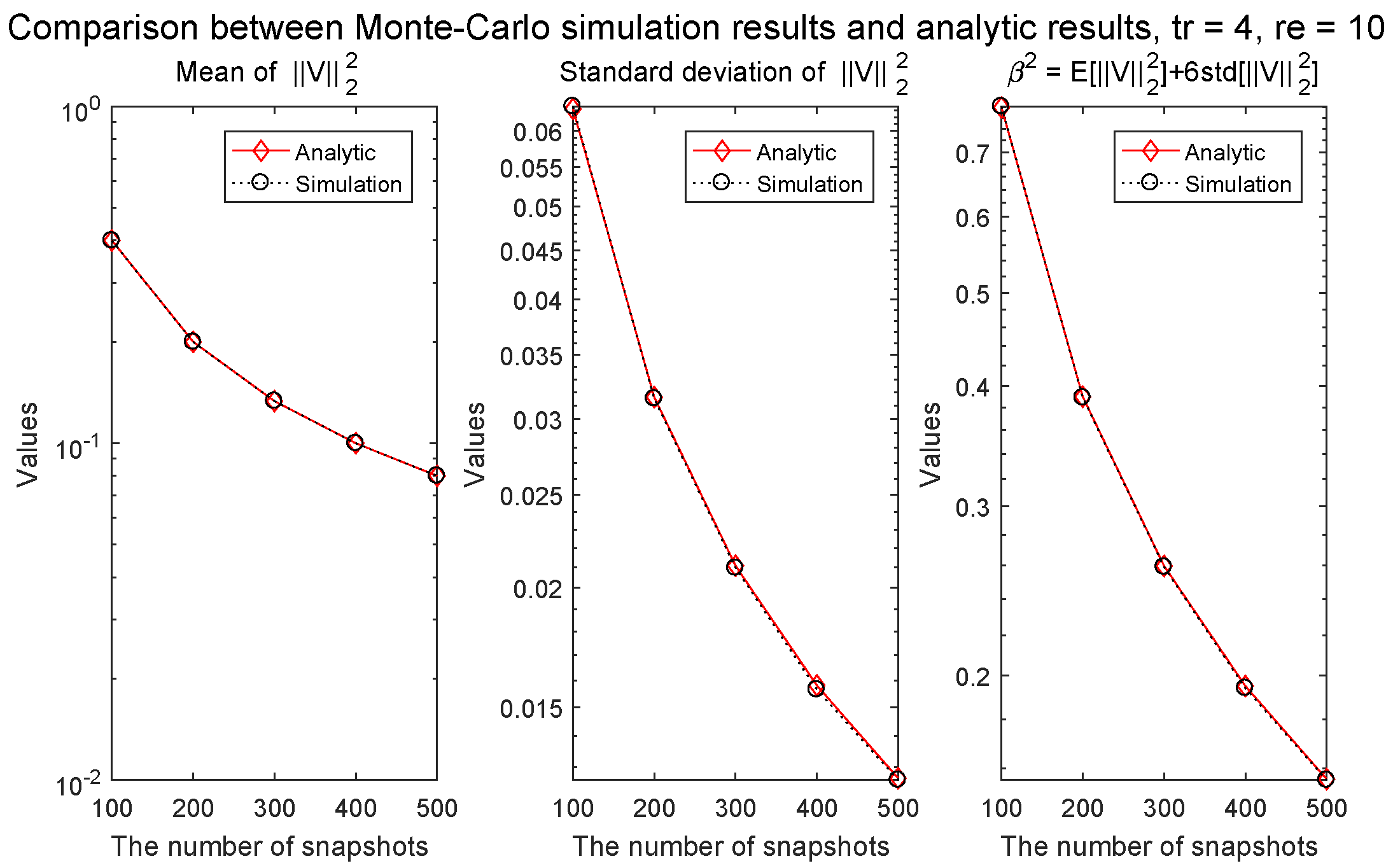
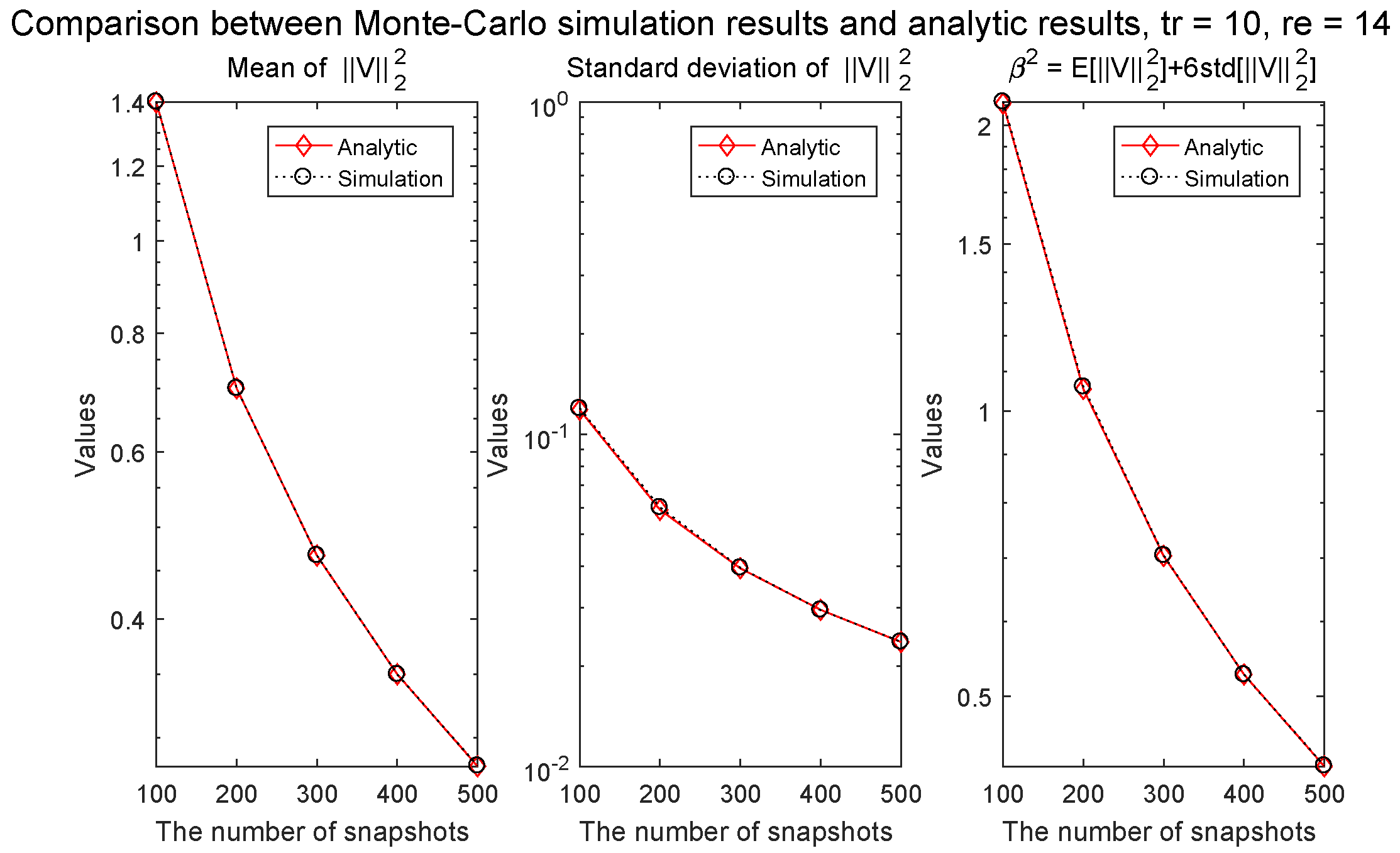
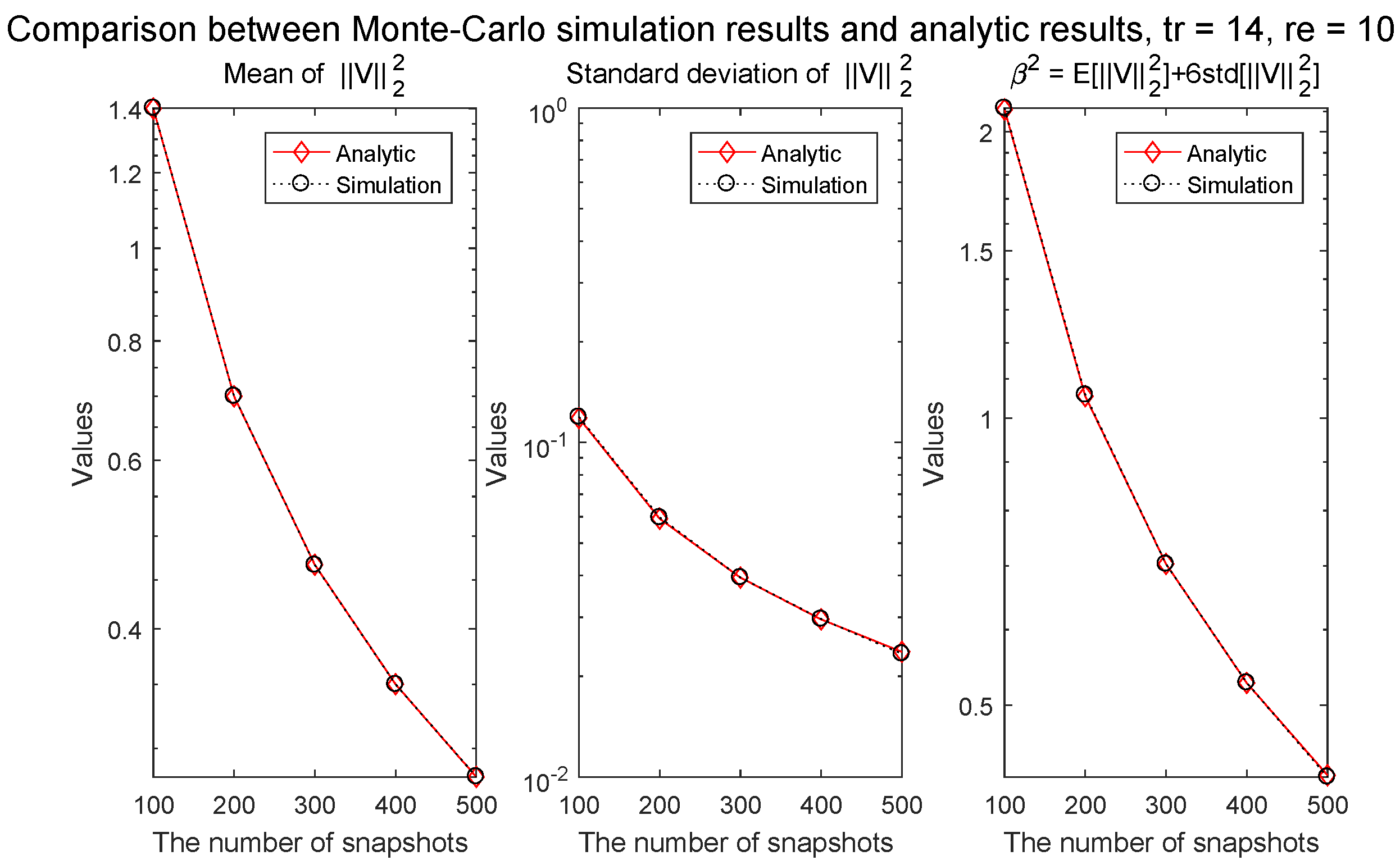
The parameter of the constraint condition is dependent on the number of transmitters, the number of receivers, and the number of snapshots. Therefore, in order to show the accuracy of the analytically derived parameter of the constraint condition, based on various cases of the three parameters, the results of the analytic derivation have been compared with results of Monte Carlo simulation. Simulations have been made 10,000 times for the Monte Carlo simulation.
Figure 3, Figure 4, Figure 5 and Figure 6 show that the mean of v 2 2 , standard derivation of v 2 2 , and the parameter of the constraint condition β 2 derived in this paper with respect to the number of snapshots when the number of elements of the transmitter and receiver are variously set. In order to show the validity of each result of the analytic derivation, the results of each analytic derivation are compared with the results obtained by the Monte Carlo simulation.
Figure 3, Figure 4, Figure 5 and Figure 6 show that the analytically derived β 2 , which is the parameter of the constraint condition, and β 2 obtained from the Monte Carlo simulation are the same for all cases. In Section 4.2, using (20) and (21), the proposed scheme has been implemented by using MATLAB to show the performance of the DOD and DOA estimation.

4.2. Performance of the Bistatic Data Fitting DOD/DOA Estimation Algorithm

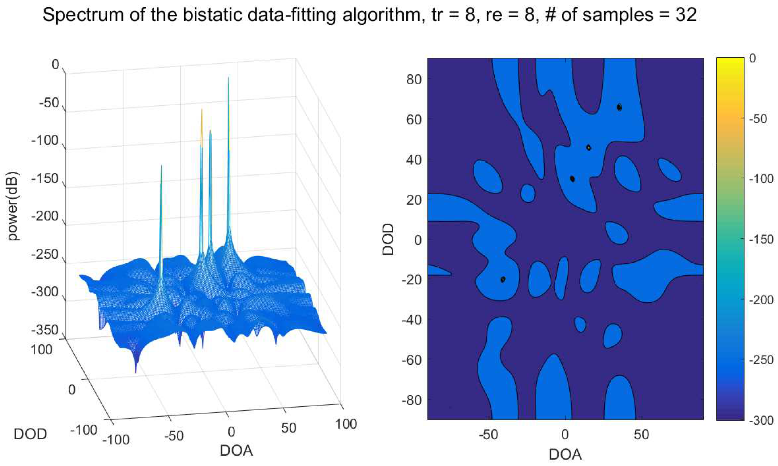
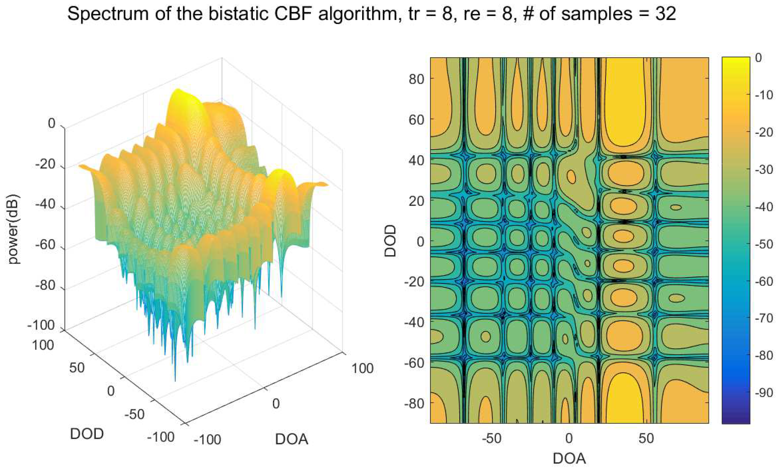
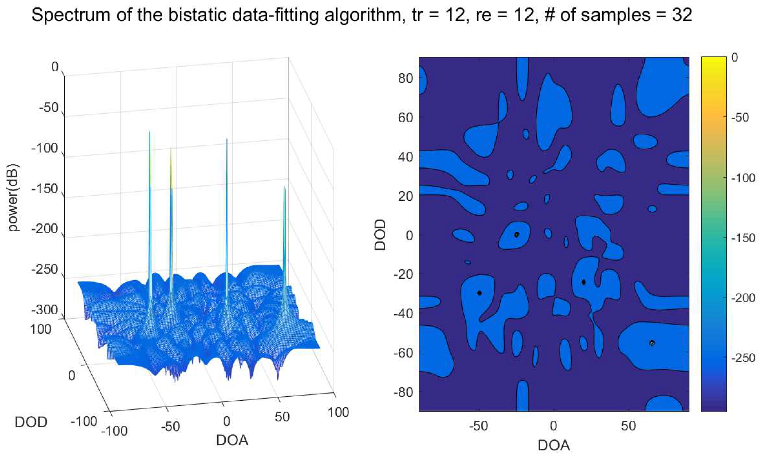
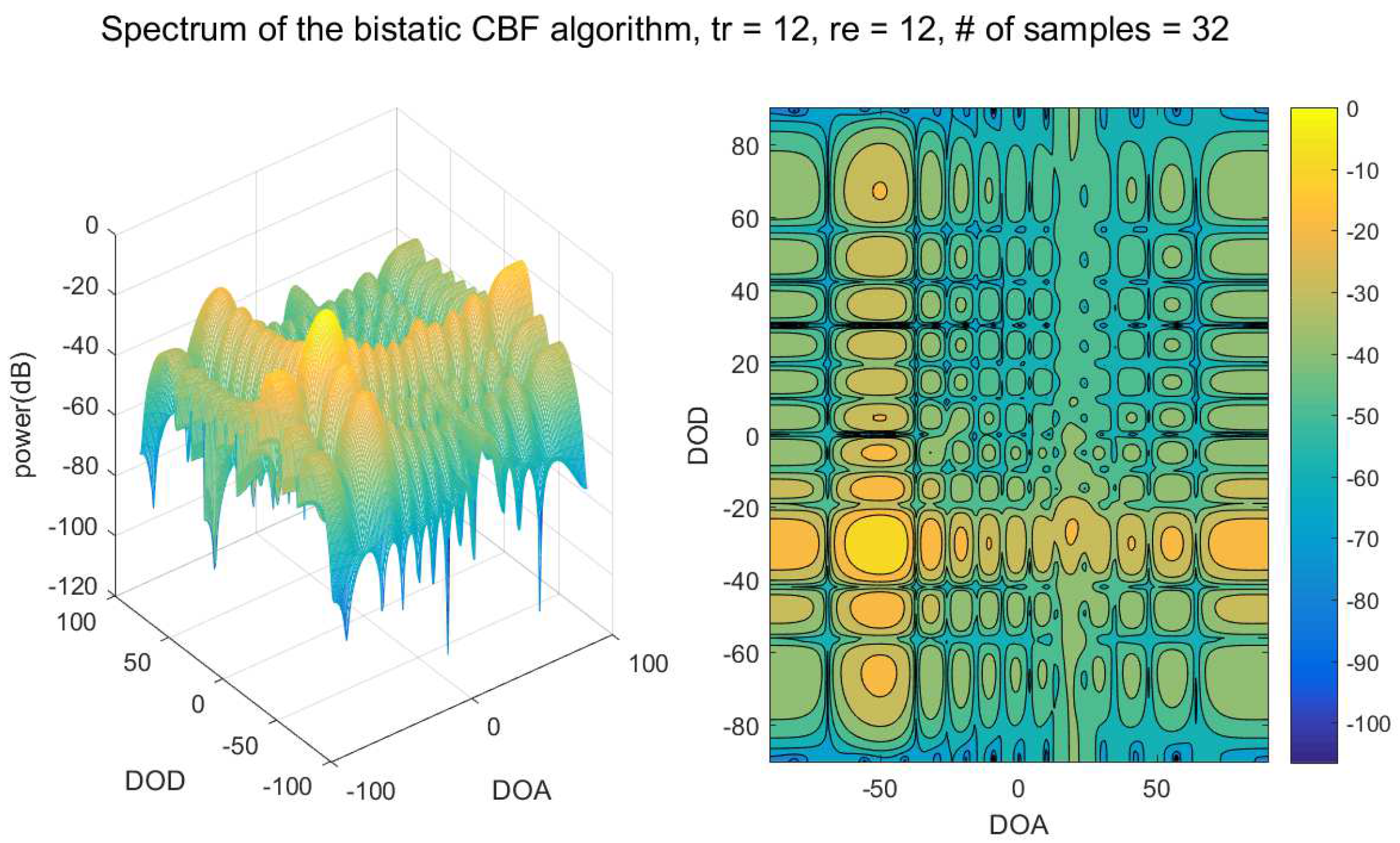
Figure 7, Figure 8, Figure 9 and Figure 10 illustrate the spectrums of the proposed scheme and the bistatic conventional beamforming method when multiple targets (more than three) exist.
Figure 7 shows the DOD/DOA estimation result of the proposed scheme based on the simulation parameters in Table 1. The number of targets is set to 4, and the SNR of each target is set differently. The figure shows that the proposed scheme accurately estimates the DODs and DOAs of the four targets.
The spectrum of the bistatic conventional beamforming algorithm based on the simulation parameters on Table 1 is illustrated in Figure 8. In the case of the beam forming method, as the main lobe and side lobe exist, the broad spectrum is usually formed. In Figure 8, it can be seen that the broad main lobe is formed around target 4, which has the highest SNR. However, due to side lobes, the DODs and DOAs of the other three targets cannot be estimated.
Figure 9 illustrates the spectrum of the proposed scheme based on the simulation parameters in Table 2. The number of targets is four, and the SNR of each target is set differently. In Figure 9, it can be seen that the proposed scheme accurately estimates the DODs and DOAs of the four targets which have different SNRs to each other.
Figure 10 shows the spectrum of the bistatic conventional beamforming algorithm based on the simulation parameters on Table 2. In Figure 10, it can be seen that broad main lobe is formed around target 1, which has the highest SNR. However, due to side lobes, the DODs and DOAs of the other three targets cannot be estimated.
The spectrum of the proposed scheme is formed into a line spectrum due to sparse recovery. Therefore, the proposed scheme has superior resolution and can accurately estimate all four targets’ DODs and DOAs. In addition, the spectrums of the proposed scheme in Figure 7 and Figure 9 prove that the parameter of the constraint condition derived in this paper are appropriate.
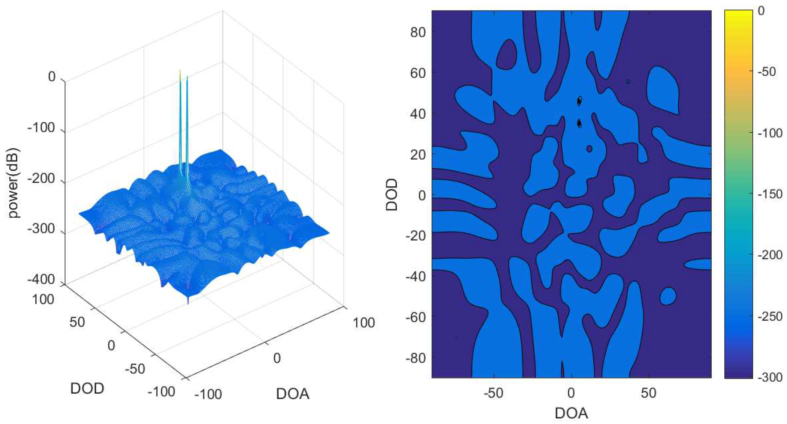
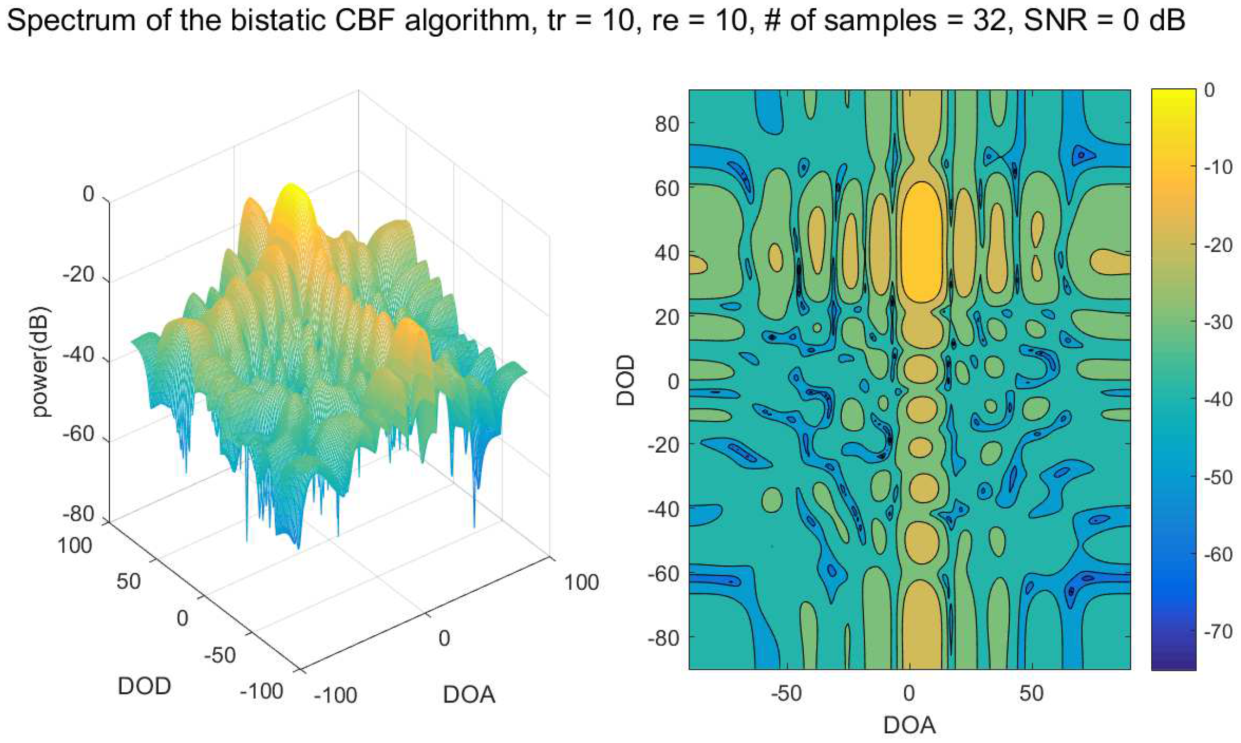
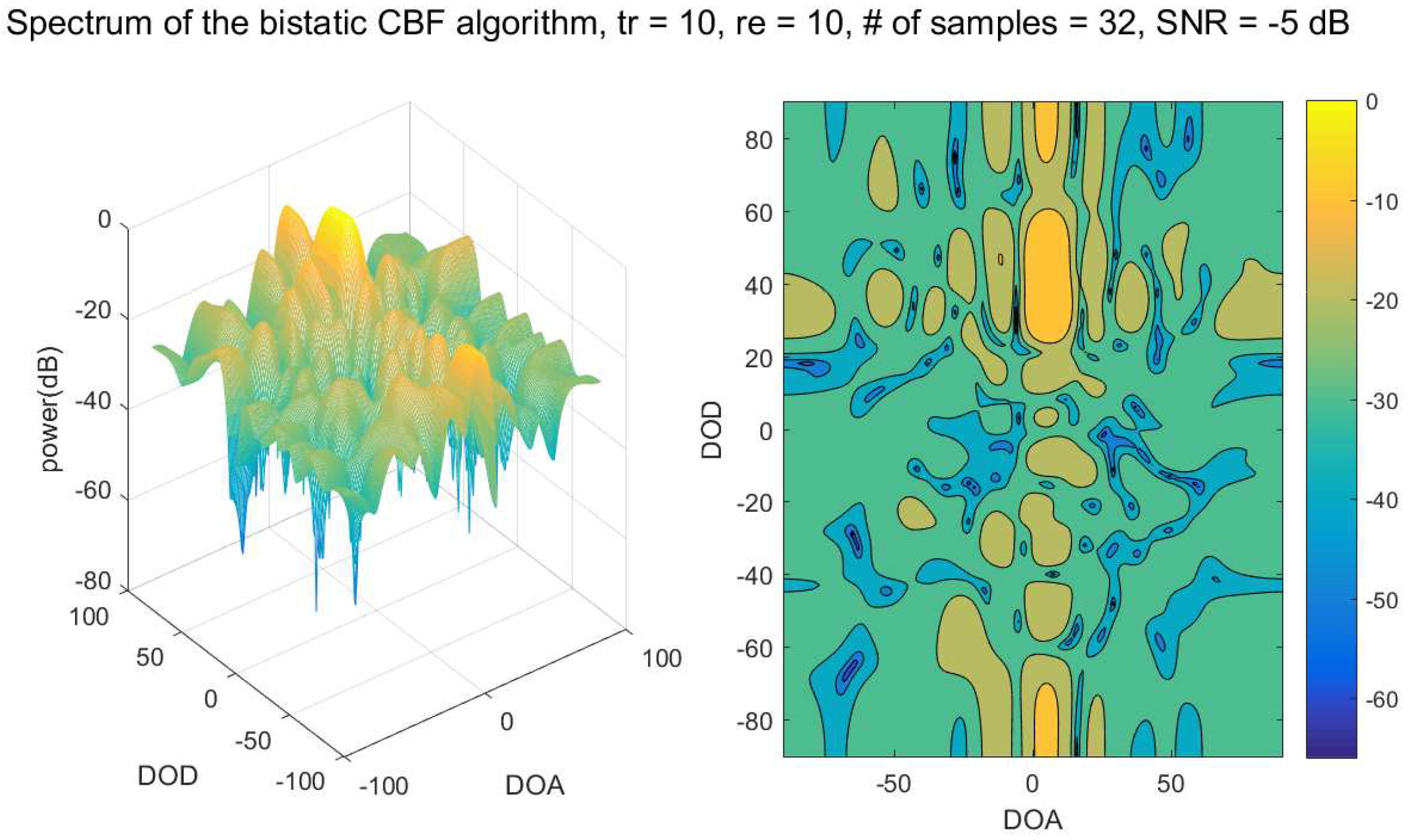
In order to clearly compare the performance of the proposed scheme and the conventional method, the simulations were conducted under poor conditions in which the SNRs were 0 and −5 dB and the locations of the two targets were very close as tabulated in Table 3.
The spectrum of the proposed DOD/DOA estimation algorithm when the SNR is 0 dB is illustrated in Figure 11. The figure shows that the proposed scheme accurately estimates the DODs and DOAs of the two adjacent targets. The difference of the noise floor and the peak values of the two targets is greater than 200 dB.
Figure 12 shows the spectrum of the conventional bistatic beamforming D0D/DOA estimation algorithm for SNR = 0 dB. Comparing Figure 11 and Figure 12, Figure 12 shows that many spurious peaks occur in this case. Moreover, unlike the proposed scheme, the conventional method shows poor resolutions that cannot resolve two adjacent targets.
In Figure 13, the spectrum of the proposed DOD/DOA estimation algorithm for SNR = −5 dB is shown. Although the SNR in Figure 13 is worse than that in Figure 11, the spectrum of Figure 13 shows that the proposed scheme accurately estimates the DODs and DOAs of the two adjacent targets. Furthermore, the difference of the noise floor and the peak values of the two targets is greater than 200 dB.
Figure 14 illustrates the spectrum of the bistatic conventional beamforming method for SNR = −5 dB. The result of Figure 14 shows that the conventional method can not estimate the DODs and DOAs of the two adjacent targets.
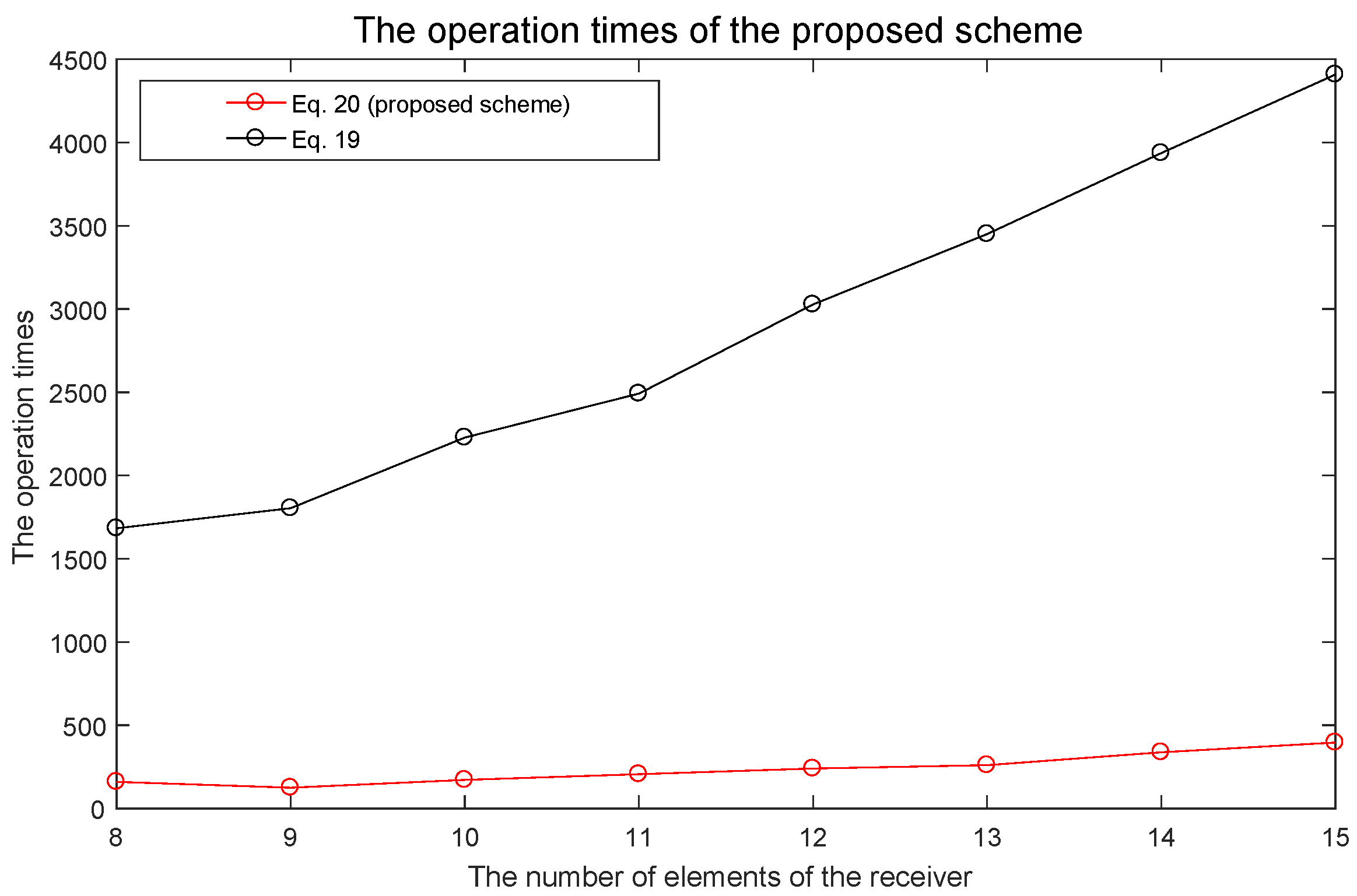
Figure 15 shows the operation times of the proposed scheme using (20); the cost function, which uses the parameter ( β 2 ) of the constraint condition derived in this paper; and the scheme using the cost function without constraint condition in (19). The operation times of the two ways depend on the number of total elements of the transmitter and receiver. The simulation parameters of Figure 15 are in Table 4.
It can be confirmed using Figure 15 that the operation times increase as the number of receivers increases both in the proposed scheme using (20) and the other scheme using (19).
In the case of the scheme using (19), as the convex optimization needs to be performed many times while changing the weight value w, it requires a large amount of computation. On the other hand, in the case of the proposed scheme using the parameter ( β 2 ) of the constraint condition derived in this paper, as the convex optimization is performed only once, the amount of computation can be minimized.
Figure 15 illustrates that using the proposed scheme in (20) is much less computationally intensive than the other scheme using the cost function in (19), which justifies why the proposed scheme using the parameter ( β 2 ) of the constraint condition should be employed for DOD/DOA estimation.

5. Conclusions

In this paper, a compressive sensing-based data fitting DOD/DOA estimation algorithm has been proposed to apply the superior performance of the compressive sensing method to the bistatic MIMO sonar systems. The proposed algorithm in this paper optimizes the output data as sparse by searching the solution through convex optimization, so that it is possible to estimate the DOD and the DOA for each target accurately.
Through simulation, the DOD/DOA estimation performance of two adjacent targets and multiple targets (more than three) has been compared with the bistatic conventional beamforming algorithm, and in all cases, the estimation performance of the proposed algorithm has been confirmed to be superior to that of the bistatic conventional beamforming algorithm.
In order to minimize the amount of computation, the cost function with constraint condition has been implemented in this paper. Furthermore, the constraint condition parameter of the cost function has been analytically derived. The validity of the parameter ( β 2 ) of the constraint condition analytically derived in this paper has been shown by comparison with the value obtained from Monte Carlo simulation. The operation times of the cost function with the constraint condition and the cost function without the constraint condition have been compared. Through the numerical result, it has been confirmed that the proposed scheme in this paper is computationally efficient.
Through various simulations, it has been shown that the proposed scheme is superior to the previous DOD/DOA estimation algorithms and that the value of the regularization parameter can be analytically derived.

Author Contributions

J.W.P. made a Matlab implementation of the proposed algorithm and formulated the proposed algorithm. J.W.P., W.H. and J.-H.L. wrote the manuscript. J.W.P. and J.-H.L. derived the results in the manuscript. All authors have read and agreed to the published version of the manuscript.

Funding

This work was supported by the Agency for Defense Development (ADD) in Korea under the Contract No. UD190005DD.

Conflicts of Interest

The authors declare no conflict of interest.

Appendix A. Parameter of the Constraint Condition β2

Appendix A.1. Mean of v 2 2

The k-th row and l-th column element of the v can be written as
v k , l = 1 L i = 1 L n k i s l i * , k = 1 , , N l = 1 , , M .
v 2 2 can be expressed as
v 2 2 = v 1 , 1 2 + v 1 , 2 2 + + v N , M 2 .
E v 2 2 can be expressed as
E v 2 2 = E v 1 , 1 2 + E v 1 , 2 2 + + E v N , M 2 .
E v k , l 2 can be expressed as
E v k , l 2 = E 1 L 2 v k , l · v k , l * = E 1 L 2 n k 1 s l 1 * + + n k L s l L * n k 1 * s l 1 + + n k L * s l L
E v k , l 2 can be expanded to a term of sum of conjugate multiplication with oneself, A, and a term of sum of conjugate multiplication with each other, B.
E v k , l 2 = E 1 L 2 A + B .
The mean of A can be obtained as follows. At first, E n k i s l i * n k i * s l i can be written as
E n k i s l i * n k i * s l i = E n k i 2 · s l i 2 = E n k Re i 2 + n k Im i 2 · s l i 2 = E n k Re i 2 + E n k Im i 2 · s l i 2 = σ 2 2 + σ 2 2 · s l i 2 = σ 2 s l i 2
Using the fact that the coded pulse matrix S is based on Hadamard code and that every L cases of conjugate multiplication with oneself has the same value, the mean of A can be achieved as
s l i 2 = 1
E A = L σ 2 s l i 2 = L σ 2 .
The mean of B can be obtained as follows. At first, E n k i s l i * n k i * s l i can be derived as
E n k i s l i * n k i * s l i = s l i * s l i E n k i n k i * = s l i * s l i E n k i E n k i * = 0
i and i denote the different indices of the snapshots to each other. Using the fact that every L 2 L cases of conjugate multiplication each other has the same value, the mean of B can be written as
E B = L 2 L · 0 = 0
Using (A8) and (A10), E v 2 2 can be derived as
E v 2 2 = M N L 2 L σ 2 = M N L σ 2

Appendix A.2. Standard Deviation of v 2 2

To evaluate the standard deviation of v 2 2 , E v 2 2 2 should be available first. E v 2 2 2 can be written as
E v 2 2 2 = E v 1 , 1 4 + E v 1 , 2 4 + + E v N , M 4 + E v 1 , 1 2 · v 1 , 2 2 + v 1 , 3 2 + + v N , M 2 + E v N , M 2 · v 1 , 1 2 + v 1 , 2 2 + + v N , M 1 2 .
To evaluate E v 2 2 2 , (A12) can be classified into two parts as follows,
Part 1 = E v 1 , 1 4 + E v 1 , 2 4 + + E v N , M 4
Part 2 = E v 1 , 1 2 · v 1 , 2 2 + v 1 , 3 2 + + v N , M 2 + E v N , M 2 · v 1 , 1 2 + v 1 , 2 2 + + v N , M 1 2

Appendix A.2.1. Part 1

(A13) can be expressed as
E v 1 , 1 4 + E v 1 , 2 4 + + E v N , M 4 = E v 1 , 1 2 2 + E v 1 , 2 2 2 + + E v N , M 2 2 .
Using (A5) in (A15), we can express E v k , l 2 2 as
E v k , l 2 2 = E 1 L 4 A + B A + B .

Derivation of E [A2]

(A17) is an example of cases of the squared term.
E n k l s k l * n k l * s k l n k l s k l * n k l * s k l = s k l 2 2 · E n k l 2 2 = s k l 2 2 · E n k Re l 2 + n k Im l 2 2 = s k l 2 2 · 2 σ 4
By using S is based on Hadamard code, (A17) can be simplified to
E n k l s k l * n k l * s k l n k l s k l * n k l * s k l = s k l 2 2 2 σ 4 L = 2 σ 4
An example of cases of the cross term of multiplication can be written as
E n k l s k l * n k l * s k l n k l s k l * n k l * s k l = E n k l 2 s k l 2 n k l 2 s k l 2 = s k l 2 s k l 2 E n k l 2 n k l 2 = s k l 2 s k l 2 E n k l 2 E n k l 2 = s k l 2 s k l 2 E n k Re l 2 + E n k Im l 2 E n k Re l 2 + E n k Im l 2 = s k l 2 s k l 2 σ 2 2 + σ 2 2 σ 2 2 + σ 2 2 = s k l 2 s k l 2 σ 4
Using s k l 2 = 1 and s k l 2 = 1 , (A19) can be simplified to
E n k l s k l * n k l * s k l n k l s k l * n k l * s k l = s k l 2 s k l 2 σ 4 = σ 4
The number of squared terms is L and the number of cross terms of multiplication is L 2 L . Therefore, E A 2 can be written as
E A 2 = 2 σ 4 L + σ 4 L 2 L

Derivation of E 2 A B

Each term of E 2 A B can be classified into three cases:
Case 1 = E n k l s k l * n k l * s k l n k l s k l * n k l * s k l Case 2 = E n k l s k l * n k l * s k l n k l s k l * n k l * s k l Case 3 = E n k l s k l * n k l * s k l n k l s k l * n k l * s k l , l l l
By using E n k l * = 0 , case 1 can be written as
E n k l s k l * n k l * s k l n k l s k l * n k l * s k l = E n k l 2 s k l 2 n k l s k l * n k l * s k l = s k l 2 s k l * s k l E n k l 2 n k l n k l * = s k l 2 s k l * s k l E n k l 2 n k l E n k l * = s k l 2 s k l * s k l E n k l 2 n k l · 0 = 0
By using E n k l = 0 , case 2 can be written as
E n k l s k l * n k l * s k l n k l s k l * n k l * s k l = E n k l 2 s k l 2 n k l s k l * n k l * s k l = s k l 2 s k l * s k l E n k l 2 n k l n k l * = s k l 2 s k l * s k l E n k l 2 n k l * E n k l = s k l 2 s k l * s k l E n k l 2 n k l * · 0 = 0
By using E n k l = 0 and E n k l * = 0 , case 3 can be written as
E n k l s k l * n k l * s k l n k l s k l * n k l * s k l = E n k l 2 s k l 2 n k l s k l * n k l * s k l = s k l 2 s k l * s k l E n k l 2 n k l n k l * = s k l 2 s k l * s k l E n k l 2 E n k l E n k l * = s k l 2 s k l * s k l E n k l 2 · 0 · 0 = 0
From (A23)– (A25), E 2 A B is identically zero for all cases:
E 2 A B = 0 .

Derivation of E B 2

There are two cases in E B 2 . The example of the first case can be written as
E n k l s k l * n k l * s k l n k l s k l * n k l * s k l = s k l * s k l 2 E n k l 2 n k l * 2 = s k l * s k l 2 E n k Re l + j n k Im l 2 E n k Re l j n k Im l 2 = s k l * s k l 2 E n k Re l 2 E n k Im l 2 E n k Re l 2 E n k Im l 2 = s k l * s k l 2 σ 2 2 σ 2 2 σ 2 2 σ 2 2 = 0
The second case can be subdivided into five cases:
Case I E n k l s k l * n k l * s k l n k l s k l * n k l * s k l Case II E n k l s k l * n k l * s k l n k l s k l * n k l * s k l Case III E n k l s k l * n k l * s k l n k l s k l * n k l * s k l Case IV E n k l s k l * n k l * s k l n k l s k l * n k l * s k l Case V E n k l s k l * n k l * s k l n k l s k l * n k l * s k l
By using s k l 2 = 1 and s k l 2 = 1 , case I can be derived as
E n k l s k l * n k l * s k l n k l s k l * n k l * s k l = s k l 2 s k l 2 E n k l 2 n k l 2 = E n k l 2 E n k l 2 = E n k Re l 2 + E n k Im l 2 E n k Re l 2 + E n k Im l 2 = σ 2 2 + σ 2 2 σ 2 2 + σ 2 2 = σ 4
As the elements of the noise matrix are independent and identically distributed (IID) random variables, the results of cases II–V in (A28) turn to zero.
The number of terms of E B 2 is L 2 L . Therefore, E B 2 can be written as
E B 2 = σ 4 L 2 L
From (A21), (A26), and (A30), (A15) is simplified to
E v 1 , 1 4 + E v 1 , 2 4 + + E v N , M 4 = M N L 4 2 L σ 4 + L 2 L σ 4 + L 2 L σ 4 = M N L 4 2 L σ 4 + 2 L 2 L σ 4 = 2 M N L 2 σ 4 L 4 .

Appendix A.2.2. Part 2

After expanding (A14), each term of (A14) can be written as
E v k , l 2 v k , l 2 = 1 L 4 E A + B A + B = 1 L 4 E A A + E A B + E B A + E B B .
(A32) can be subdivided into four cases of E A A , E A B , E B A , and E B B .
For k = k
It can be shown that E v k , l 2 v k , l 2 is constant as long as k is equal to k irrespective of whether l is equal to l or not. For example, for evaluating E v 1 , 1 2 v 1 , 2 2 + v 1 , 3 2 + + v N , M 2 , we can use
E v 1 , 1 2 v 1 , 1 2 = E v 1 , 1 2 v 1 , 2 2 = = E v 1 , 1 2 v 1 , M 2 .
The number of these terms is M M 1 for k k = 1 , , N -th sensor.
By using (A21) and (A26), E A A , E A B , E B A of E v k , l 2 v k , l 2 for k = k , l = l and k = k , l l can be simplified to
E A A = 2 L σ 4 + L 2 L σ 4
E A B = E B A = 0 .
In the case of E B B , terms of coded pulse’s elements are not 1. It can be shown as
E n k l s k l * n k l * s k l n k l s k l * n k l * s k l = s k l * s k l s k l * s k l E n k l n k l * n k l n k l * = s k l * s k l s k l * s k l E n k l 2 n k l 2 = s k l * s k l s k l * s k l σ 4 , s k l * s k l s k l * s k l 1 .
l takes L 1 values of 1 , , l 1 , l + 1 , , L . When l is fixed and the number of snapshots, L, is even, the sum of L 1 cases of s k l * s k l s k l * s k l is 1 . For even l and odd L, the sum of L 1 cases of s k l * s k l s k l * s k l is 2 . For odd l and odd L, the sum of L 1 cases of s k l * s k l s k l * s k l is 0. l can take L values of 1 , , L . E B B can be written as
E B B = L σ 4 , for even L 2 · round L / 2 σ 4 , for odd L .
The sum of M N M 1 terms of (A14) can be derived as
M N L 4 2 L σ 4 + L 2 L σ 4 L σ 4 M 1 , for even L M N L 4 2 L σ 4 + L 2 L σ 4 2 · round L / 2 σ 4 M 1 , for odd L .
For k k
For k k , (A38), an example case of the remaining E A A of (A32) can be written as
E n k l 2 s k l 2 n k l 2 s k l 2 = s k l 2 s k l 2 E n k l 2 n k l 2 = E n k l 2 E n k l 2 = σ 2 / 2 + σ 2 / 2 σ 2 / 2 + σ 2 / 2 = σ 4 .
The number of terms is L 2 . The E A A for k k can be written as
E A A = L 2 σ 4 .
Expectation of a term in E A B and E B A For k k can be written as
E n k l 2 s k l 2 n k l s k l * n k l * s k l = s 1 1 2 s k l * s k l E n k l 2 n k l n k l * = s 1 1 2 s k l * s k l E n 1 1 2 E n k l E n k l = 0 .
Expected value of a term in E B B of (A32) For k k can be written as
E n k l s k l * n k l * s k l n k l s k l * n k l * s k l = s k l * s k l s k l * s k l E n k l n k l * n k l n k l * = s k l * s k l s k l * s k l E n k l E n k l * E n k l E n k l * = 0 .
The sum of terms of (A14) for k k can be given as
Part 2 for k k = M N L 4 M * N 1 M 1 L 2 σ 4 .
Part 2 of (A14) can be given as
Part 2 = M N L 4 ( 2 L σ 4 + ( L 2 L ) σ 4 L σ 4 ) M 1 + M N L 4 M * N 1 M 1 L 2 σ 4 .
By using (A31) and (A44) the mean of v 2 2 2 can be derived as
E v 2 2 2 = 2 M N L 2 σ 4 L 4 + M N L 4 ( 2 L σ 4 + ( L 2 L ) σ 4 L σ 4 ) M 1 + M N L 4 M * N 1 M 1 L 2 σ 4 .
Using (A11) and (A45), the variance of v 2 2 can be achieved as
var v 2 2 = E v 2 2 2 E v 2 2 2
Using (A46), the standard deviation of v 2 2 can be achieved as
std v 2 2 = var v 2 2 1 2

References

  1. Krim, H.; Viberg, M. Two decades of array signal processing research—The parametric approach. IEEE Signal Process. Mag. 1996, 13, 67–94. [Google Scholar] [CrossRef]
  2. Capon, J. High resolution frequency-wavenumber spectrum analysis. Proc. IEEE 1969, 57, 1408–1418. [Google Scholar] [CrossRef] [Green Version]
  3. Schmidt, R.O. Multiple emitter location and signal parameter estimation. IEEE Trans. Antennas Propag. 1986, 34, 276–280. [Google Scholar] [CrossRef] [Green Version]
  4. Malioutov, D.; Cetin, M.; Willsky, A. A sparse signal reconstruction perspective for source localization with sensor arrays. IEEE Trans. Signal Process. 2005, 53, 3010–3022. [Google Scholar] [CrossRef] [Green Version]
  5. Mohimani, H.; Babaie-Zadeh, M. A Fast Approach for Overcomplete Sparse Decomposition Based on Smoothed l0 Norm. IEEE Trans. Signal Process. 2009, 57, 289–301. [Google Scholar] [CrossRef] [Green Version]
  6. Zheng, J.; Kaveh, M.; Tsuji, H. Sparse spectral fitting for direction of arrival and power estimation. In Proceedings of the 2009 IEEE/SP 15th Workshop on Statistical Signal Processing, Cardiff, UK, 31 August–3 September 2009. [Google Scholar]
  7. Picard, J.; Weiss, A. Direction finding of multiple emitters by spatial sparsity and linear programming. In Proceedings of the 2009 9th International Symposium on Communications and Information Technology (ISCIT), Icheon, Korea, 28–30 September 2009; pp. 1258–1262. [Google Scholar]
  8. Zheng, J.; Kaveh, M. Directions-of-arrival estimation using a sparse spatial spectrum model with uncertainty. In Proceedings of the 2011 IEEE International Conference on Acoustics, Speech and Signal Processing (ICASSP’11), Prague, Czech Republic, 22–27 May 2011. [Google Scholar]
  9. Stoica, P.; Babu, P.; Li, J. Spice: A sparse covariance-based estimation method for array processing. IEEE Trans. Signal Process. 2011, 59, 629–638. [Google Scholar] [CrossRef]
  10. Zheng, J.; Kaveh, M. Sparse Spatial Spectral Estimation: A Covariance Fitting Algorithm, Performance and Regularization. IEEE Trans. Signal Process. 2013, 61, 2767–2777. [Google Scholar] [CrossRef]
  11. Paik, J.W.; Hong, W.; Ahn, J.-K.; Lee, J.-H. Statistics on noise covariance matrix for covariance fitting-based compressive sensing direction-of-arrival estimation algorithm: For use with optimization via regularization. J. Acoust. Soc. Am. 2018, 143, 3883–3890. [Google Scholar] [CrossRef] [PubMed]
  12. Liu, L.; Zhang, X.; Chen, P. Compressed Sensing-Based DOA Estimation with Antenna Phase Errors. Electronics 2019, 2019, 294. [Google Scholar] [CrossRef] [Green Version]
  13. Salama, A.A.; Ahmad, M.O.; Swamy, M.N.S. Compressed Sensing DOA Estimation in the Presence of Unknown Noise. Prog. Electromagn. Res. C 2020, 102, 47–62. [Google Scholar] [CrossRef]
  14. Jin, M.; Liao, G.; Li, J. Joint DOD and DOA estimation for bistatic MIMO radar. Signal Process. 2009, 89, 244–251. [Google Scholar] [CrossRef]
  15. Liu, F.; Wang, J. AD-MUSIC for jointly DOA and DOD Estimation in Bistatic MIMO Radar System. In Proceedings of the International Conference on Computer Design and Appliations (ICCDA 2010), Qinhuangdao, China, 25–27 June 2010. [Google Scholar]
  16. Li, L.; Chen, F.; Dai, J. Separate DOD and DOA Estimation for Bistatic MIMO Radar. Int. J. Antennas Propag. 2016, 2016. [Google Scholar] [CrossRef] [Green Version]
  17. Chen, J.L.; Gu, H.; Su, W.M. A new method for joint DOD and DOA estimation in bistatic MIMO radar. Signal Process. 2010, 90, 714–718. [Google Scholar] [CrossRef]
  18. Zheng, G.; Tang, J. DOD and DOA estimation in bistatic MIMO radar for nested and coprime array with closed-form DOF. Int. J. Electron. 2017, 104, 885–897. [Google Scholar] [CrossRef]
  19. Ali, H.; Ahmad, S.; Sharawi, M.S.; Alouini, M.S. Reduced complexity DOA and DOD estimation for a single moving target in bistatic MIMO radar. Signal Process. 2019, 166, 1–11. [Google Scholar] [CrossRef]
  20. Chen, Z.; Chen, P. Compressed sensing-based DOA and DOD estimation in bistatic co-prime MIMO arrays. In Proceedings of the 2017 IEEE Conference on Antenna Measurements and Applications (CAMA), Ibaraki, Japan, 4–6 December 2017. [Google Scholar]
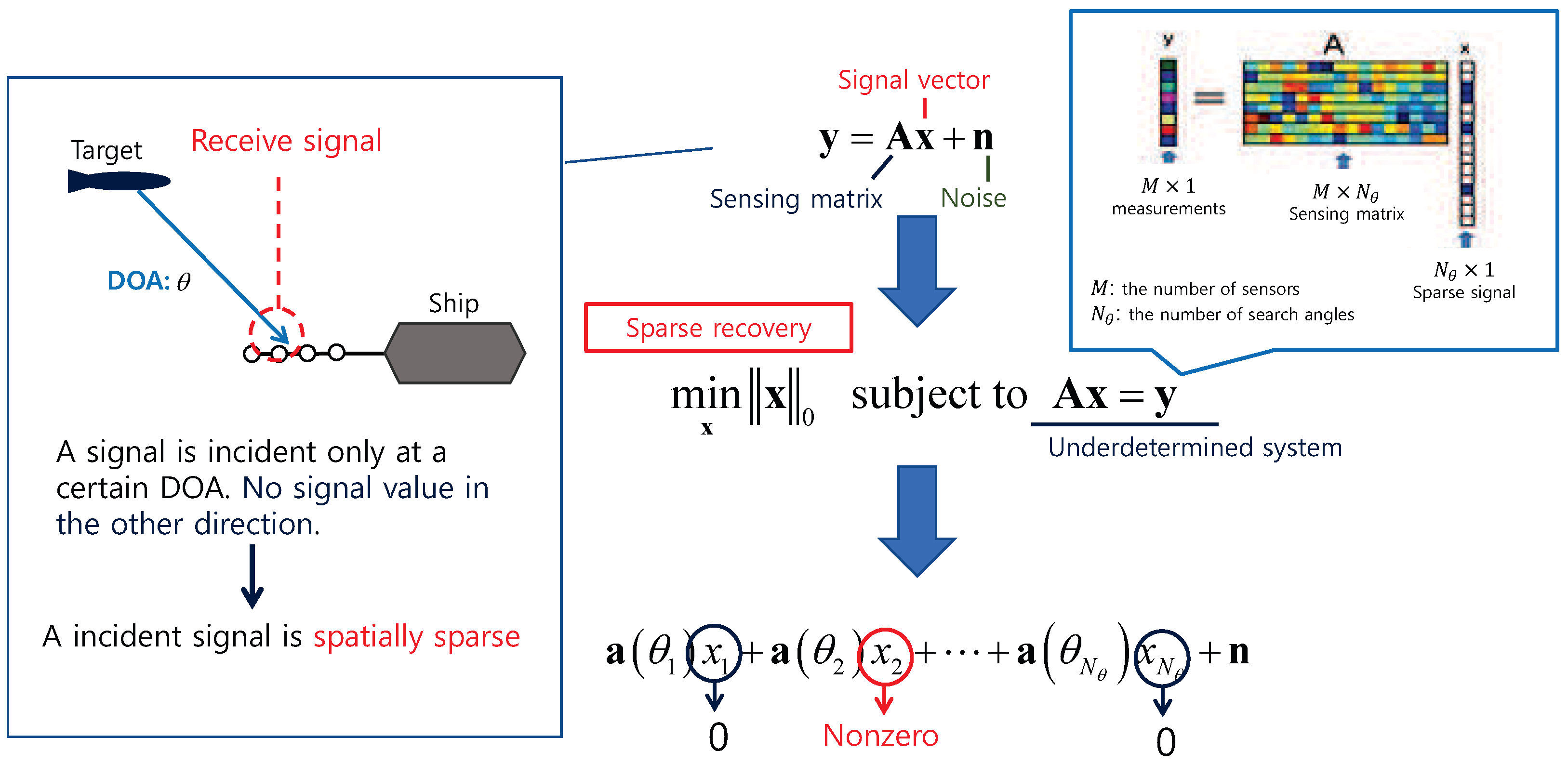
Figure 1. The concept of the compressive sensing-based DOA estimation method.
Remotesensing 12 02773 g001
Figure 2. The simulation structure based on the bistatic multiple input multiple output (MIMO) system.
Remotesensing 12 02773 g002
Figure 3. Comparison between the results of the analytic derivation and the results of Monte Carlo simulation (the number of elements of the transmitter = 4, the number of elements of the receiver = 10).
Remotesensing 12 02773 g003
Figure 4. Comparison between the results of the analytic derivation and the results of Monte Carlo simulation (the number of elements of the transmitter = 10, the number of elements of the receiver = 14).
Remotesensing 12 02773 g004
Figure 5. Comparison between the results of the analytic derivation and the results of Monte Carlo simulation (the number of elements of the transmitter = 12, the number of elements of the receiver = 12).
Remotesensing 12 02773 g005
Figure 6. Comparison between the results of the analytic derivation and the results of Monte Carlo simulation (the number of elements of the transmitter = 14, the number of elements of the receiver = 10).
Remotesensing 12 02773 g006
Figure 7. Spectrum of the bistatic data fitting algorithm, the number of targets = 4 (case 1).
Remotesensing 12 02773 g007
Figure 8. Spectrum of the bistatic conventional beamforming algorithm, the number of targets = 4 (case 1).
Remotesensing 12 02773 g008
Figure 9. Spectrum of the bistatic data fitting algorithm, the number of targets = 4 (case 2).
Remotesensing 12 02773 g009
Figure 10. Spectrum of the bistatic conventional beamforming algorithm, the number of targets = 4 (case 2).
Remotesensing 12 02773 g010
Figure 11. Spectrum of the bistatic data fitting DOD/DOA estimation algorithm, SNR = 0 dB.
Remotesensing 12 02773 g011
Figure 12. Spectrum of the bistatic conventional beamforming algorithm, SNR = 0 dB.
Remotesensing 12 02773 g012
Figure 13. Spectrum of the bistatic data fitting DOD/DOA estimation algorithm, SNR = −5 dB.
Remotesensing 12 02773 g013
Figure 14. Spectrum of the bistatic conventional beamforming algorithm, SNR = −5 dB.
Remotesensing 12 02773 g014
Figure 15. The operation times Comparison between the proposed scheme using the parameter ( β 2 ) of the constraint condition and the other scheme without using the constraint condition.
Remotesensing 12 02773 g015
Table 1. Simulation parameters of multiple targets (case 1).
ParameterValue
The number of elements of the transmitter8
The number of elements of the receiver8
The number of samples32
The number of targets4
The wavelength 0.03 m
Inter-elements spacing at the receiver 0.5 wavelength
Inter-elements spacing at the transmitter 0.5 wavelength
Search range of DOD and DOA 90 : 1 : 90
True DOD and DOA of the target 1 (SNR = −5 dB) 20 , 40
True DOD and DOA of the target 2 (SNR = 15 dB) 30 , 5
True DOD and DOA of the target 3 (SNR = 0 dB) 45 , 15
True DOD and DOA of the target 4 (SNR = 25 dB) 65 , 35
Table 2. Simulation parameters of multiple targets (case 2).
ParameterValue
The number of elements of the transmitter12
The number of elements of the receiver12
The number of samples32
The number of targets4
The wavelength 0.03 m
Inter-elements spacing at the receiver 0.5 wavelength
Inter-elements spacing at the transmitter 0.5 wavelength
Search range of DOD and DOA 90 : 1 : 90
True DOD and DOA of the target 1 (SNR = 25 dB) 30 , 50
True DOD and DOA of the target 2 (SNR = 15 dB) 25 , 20
True DOD and DOA of the target 3 (SNR = −5 dB) 55 , 65
True DOD and DOA of the target 4 (SNR = 5 dB) 0 , 25
Table 3. Simulation parameters for two adjacent targets.
ParameterValue
The number of elements of the transmitter10
The number of elements of the receiver10
The number of samples32
The number of targets2
The wavelength 0.03 m
Inter-elements spacing at the receiver 0.5 wavelength
Inter-elements spacing at the transmitter 0.5 wavelength
Search range of DOD and DOA 90 : 1 : 90
True DOD and DOA of the target 1 35 , 5
True DOD and DOA of the target 2 45 , 5
Table 4. Simulation parameters for the operation time comparison.
ParameterValue
The number of elements of the transmitter8
The number of elements of the receiver8:15
The number of samples32
The number of targets4
The wavelength 0.03 m
The number of weight parameters ( w ) 10
Inter-elements spacing at the receiver 0.5 wavelength
Inter-elements spacing at the transmitter 0.5 wavelength
Search range of DOD and DOA 90 : 1 : 90