Comparative Analysis of the Effect of the Loading Series from GFZ and EOST on Long-Term GPS Height Time Series

Abstract

In order to investigate the effect of different loading models on the nonlinear variations in Global Positioning System (GPS) height time series, the characteristics of annual signals (amplitude and phase) of GPS time series, loading series from Deutsche GeoForschungsZentrum, Germany (GFZ) and School and Observatory of Earth Sciences, France (EOST) at 633 global GPS stations are processed and analyzed. The change characteristics of the root mean square (RMS) reduction rate, annual amplitude and phase of GPS time series after environmental loading corrections (ELCs) are then detected. Results show that ELCs have a positive effect on the reduction in the nonlinear deformation contained in most GPS stations around the world. RMS reduction rates are positive at 82.6% stations after GFZ correction and 87.4% after EOST correction, and the average reduction rates of all stations are 10.6% and 15.4%, respectively. As for the environmental loading series from GFZ and EOST, their average annual amplitudes are 2.7 and 3.1 mm, which explains ~40% annual amplitude of GPS height time series (7.2 mm). Further analysis of some specific stations indicates that the annual phase difference between GPS height time series and the environmental loading series is an important reason that affects the reduction rates of the RMS and annual amplitude. The linear relationship between the annual phase difference and the annual amplitude reduction rate is significant. The linear fitting results show that when there is no annual phase difference between GPS and loading series, the reduction rates of the RMS and annual amplitude will increase to the maximum of 15.6% and 41.6% for GFZ, and 22.0% and 46.6% for EOST.

1. Introduction

In recent two decades, many researchers have undertaken various topics on earth science by means of Global Positioning System (GPS) time series obtained from continuous GPS (CGPS) stations, including analysis of periodic signals [1,2,3,4,5], detection of stochastic models [6,7,8,9], spatial filtering methods [10,11,12,13,14], and surface loading models (SLMs) [15,16,17,18,19,20,21,22,23].

Existing research results indicate that land mass redistribution is one of the principal causes of the nonlinear motion in GPS time series. By establishing SLMs (including atmospheric loading, nontidal oceanic loading, hydrological loading, etc., and together referred as environmental loadings) and computing the displacement series derived from elastic deformation, effects of geophysical signals on certain GPS stations can be acquired and studied effectively. Characteristic changes of long-term GPS time series before and after the correction of environmental loadings are then compared and analyzed to detect the influence of these loadings, which is helpful to further understand the nonlinear changes included in GPS time series.

van Dam et al. [15] analyzed GPS height time series of 19 stations in the northern hemisphere, and concluded that when atmospheric loading was applied, the total variance of the GPS series could be reduced by 24%, and the atmospheric loading series fluctuated more at higher latitudes. van Dam et al. [17] also found that the nonlinear motion in GPS height time series would be better explained when the influence of unmodeled topographic variability on surface pressure estimates was taken into account. Jiang et al. [19] analyzed the causes of the nonlinear variations in the GPS time series of 11 IGS stations in China. They believed that after environmental loading corrections (ELCs, including atmospheric loading, nontidal oceanic loading, snow and soil moisture loading), the annual amplitude of GPS height series could be effectively weakened, while the effect of ELCs on the horizontal components (north and east) could not.

In the last two years, the effect of ELCs is still a heated topic. Yuan et al. [22] analyzed 235 Crustal Movement Observation Network of China (CMONOC) stations for the nonlinear motion at GPS stations. They calculated the displacement series caused by environmental loadings (including atmospheric loading, nontidal oceanic loading and hydrological loading) and found that after ELCs, the average root mean square (RMS) of GPS height time series could be reduced by ~20%. Andrei et al. [24] reported on the consistent and homogeneous data processing and analysis of a 15 year long time series of ABOA, a Finnish Antarctic research station. Then, they compared the loading series from three service providers GFZ, EOST and International Mass Loading Service (IML), and an obvious difference was found in the nontidal oceanic loading (NTOL) between GFZ and EOST. Li et al. [25] computed the land surface displacements derived from five atmospheric products and compared them with the position time series at 596 global GNSS stations. Results showed that the ERA-Interim model performs best in reducing the scatter of GNSS time series, and the ELC effect at inland stations is better than island stations for all five models. Li et al. [26] investigated the performance of different loading products on the RMS reduction in GNSS time series at CMONOC stations. They concluded that the difference in RMS reduction can reach 20% in the vertical component according to different ELCs applied.

The time span of GPS time series influences noise models, while a long-term series helps to reduce the influence of different noise models on uncertainties of the estimated parameters [27,28]. As the observation data of global GPS stations continue to accumulate, time spans of GPS time series obtained after data processing also increase. Therefore, it is necessary to re-evaluate the parameters of global long-term GPS time series to promote further understanding of the earth surface variation with more accuracy. On the other hand, although the nonlinear motion contained in the GPS time series cannot be completely eliminated by geophysical model corrections, the modeled loading corrections at different GPS stations are quite different. Many previous studies focused on the study of SLMs and the analysis of the ELC effect, while further exploration about why the ELCs perform differently among GPS stations is also important.

Apart from the application in establishing the global terrestrial reference frame, GPS time series can also be applied in some regional geodynamics studies, such as earthquakes, landslides, subsidence and volcanoes. GPS stations located in these geodynamics processes contain not only long-term displacements caused by crustal movement and environmental loadings but also some short-term local variations produced by seismic or volcanic activities. Although both lines of research require different temporal resolutions and time spans of GPS data, it provides an effective method in geodynamics research if the GPS time series keeps a consistent high temporal resolution. The main purpose of this paper was to compare loading products from GFZ and EOST, and detect their effect on the characteristic changes of global GPS height time series; then, to further explore the causes of the annual amplitude and phase differences between the observed and modeled displacement series. Based on 20 year GPS height time series of the globally distributed 633 stations and surface loading data provided by GFZ and EOST, environmental loading effects on GPS height time series of these stations were analyzed, mainly including the spatial distribution characteristics and change of RMS reduction rate, annual amplitude and phase change before and after ELCs. The influence of the colored noise combination, white noise and power law noise (WN+PL) was taken into account, which helped to accurately estimate parameters in the deterministic model of GPS time series. The reason for the large differences in the effect of ELCs on some specific stations was mainly studied. Finally, the relationship between the annual phase difference (between GPS height time series and the environmental loading series), RMS and annual amplitude reduction rate were linearly fitted to obtain the functions between them.

2. Data and Methodology

2.1. GPS Height Time Series

GPS data were obtained from Scripps Orbit and Permanent Array Center (SOPAC), one of the data analysis centers of the International GNSS Service (IGS). The data set included raw and processed GPS time series results. The SOPAC products mainly used in this paper are the linearized mean series after removing the offsets (coseismic or noncoseismic) and outliers, and maintaining the seasonal periodic signals in order to analyze the impact of environmental loadings. More detailed descriptions about the GPS postprocessing and coordinate time series can be found at the SOPAC website—http://sopac-csrc.ucsd.edu/index.php/gambit-globk/.

Before data analysis, it is necessary to select GPS stations according to data quality. The first selection criterion is that the effective time span of a GPS station in two decades (1999~2018) needs to be greater than 5 years, and 705 stations meet this demand from all 1147 stations. The second is that there are no dramatic abnormal variations, including variations caused by large postseismic deformations, single-station-related deformations and others from unknown reasons. We inspect these stations one by one and delete 39 unsatisfactory stations with 666 stations remaining. Third, in order to combine the GPS stations from SOPAC with the loading series of ~6500 stations worldwide from the EOST dataset, we acquire 633 common stations, as shown in Figure 1. The datasets we acquired from SOPAC already excluded most of the stations affected by large earthquakes, and this is expressed by the rare stations along the western coast of the United States where earthquakes happen frequently.

2.2. Environmental Loading Data

Mass redistribution of atmosphere, oceans and terrestrial water storage can cause changes in surface mass loading, resulting in displacements on the Earth’s crust [29,30], which can be called environmental loading deformation. Based on different geophysical observations and earth models, SLMs can be established to evaluate the influence on the nonlinear displacement of GPS stations [22].

Different organizations and institutes provide products of environmental loading displacement, including GFZ [31,32] in Germany, EOST (http://loading.u-strasbg.fr/, [33]) Loading Service from University of Strasbourg in France and the Global Geophysical Fluids Center (GGFC, https://geophy.uni.lu/) established by the International Earth Rotation and Reference Systems Service (IERS). Using the environmental loading products provided by GFZ and EOST, this paper estimated displacement series in 633 global GPS stations, and then deducts these displacement series from GPS height time series, so as to analyze the ELC effect derived from products of different organizations.

GFZ provides elastic deformation data of the global land surface derived from atmospheric loading (NTAL), nontidal oceanic loading (NTOL) and hydrological loading (HYDL) on a 0.5 × 0.5° regular global grid, with temporal resolutions of 3 (for NTAL and NTOL) and 24 h (for HYDL). The input geographical data that GFZ adopt to produce products of NTAL, NTOL and HYDL are, respectively, from the European Centre for Medium-Range Weather Forecasts (ECMWF), the Max-Planck Institute Ocean Model (MPIOM, [34]) and the Land Surface Discharge Model (LSDM, [35]). Based on these loading deformation grid data, a bicubic interpolation method was used to obtain displacement series at each station. In order to unify their temporal resolutions, NTAL and NTOL series with 3 h intervals were averaged into daily results. When calculating the sum loading (SUML) series, firstly, we added grid data of the above three loadings, then used the same interpolation method to obtain the SUML series so as to reduce the accuracy loss caused by more interpolations.

EOST provides models of 3D surface displacements, surface gravity and tilt variations at ~6500 global stations, computed using atmospheric, oceanic and hydrological general circulation models. The NTAL loading series employed in this paper were calculated from datasets of ECMWF Reanalysis with a temporal resolution of 6 h (ERA-Interim, [36]). This NTAL model runs from 1979 to present and is updated once per month. The spatial resolution of ERA-Interim is 0.75° in longitude and latitude. This model assumes an inverted barometer ocean response to pressure forcing in model establishment. HYDL loading series were estimated from the MERRA2 model [37] with a temporal resolution of 1 h. The output of the MERRA2 model is a regular 0.625 × 0.5° in longitude by latitude grid data [25]. This hydrological model considers soil moisture and snow depth. The NTOL loading series were estimated from the Estimating the Circulation and Climate of the Ocean Phase II (ECCO2, [38]) ocean bottom pressure with a temporal resolution of 24 h and spatial resolutions of 0.25°. Detailed information about the loading model difference between GFZ and EOST can be found in Li et al. [26].

2.3. Methodology

GPS time series can be expressed as the sum of deterministic and stochastic models [39]. The former consists of polynomial, seasonal signals (annual and semi-annual) and offsets. The stochastic model is commonly known as noises. The functional model of the GPS time series can be expressed as follows:

$$x(t)={\displaystyle \sum _{i=0}^{n_p}{p}_i(t-t_R}{)}^i+{\displaystyle \sum _{j=i}^{n_b}{b}_j}H(t-t_j)+{\displaystyle \sum _{k=1}^{n_A}{A}_k}\sin ({\omega }_{k}t+{\phi }_k)+{\displaystyle \sum _{k=1}^{n_L}{a}_k\log (1+(t-t_k)}/T_k)+\epsilon$$

(1)

where p_i is the coefficient of n_p degree polynomial; t is the epoch of the GPS time series; t_R is the reference epoch; H(t) is the Heaviside step function used to model offsets with amplitudes b_j; n_b is the number of offsets and t_j are the epochs of these offsets; A_k, w_k and φ_k are the amplitudes, angular velocities and initial phases of periodic signals, respectively; n_A is the number of periodic signals, k = 1 for annual signal and k = 2 for semi-annual signal; n_L is the number of logarithmic functions used to model postseismic deformation; a_k and T_k are two parameters of the logarithmic function; t_k is the epoch of earthquakes that caused logarithmic displacement; ε is the residual series that can be expressed as a combination of varied noise models.

In this paper, we assumed that the polynomial degree was one which is commonly used. Offsets and postseismic deformations of the GPS time series were excluded from the SOPAC products. As for the stochastic models, Hector software [40] was used to estimate the amplitude and phase of the periodic signals in the GPS height time series. This software, like the same type of CATS software [41], is based on maximum likelihood estimation, while the improved algorithms have fastened the computational speed [42]. Therefore, when estimating the periodic signals, we used the noise combination WN+PL as the noise model of the residual series, and it could simultaneously estimate the noninteger spectral index of the residual series.

When assessing the impact of ELCs on GPS height time series, the RMS reduction rate was used as an indicator, expressed as:

$$RM{S}_{reduction}=\frac{RM{S}_{GPS}-RM{S}_{GPS-SUML}}{RM{S}_{GPS}}$$

(2)

In the same way, after deducting the environmental loadings, annual amplitude and phase of GPS height time series also change along with the RMS reduction rate. Annual amplitude reduction rate is expressed as:

$$AM{P}_{reduction}=\frac{AM{P}_{GPS}-AM{P}_{GPS-SUML}}{AM{P}_{GPS}}$$

(3)

3. Results and Analysis

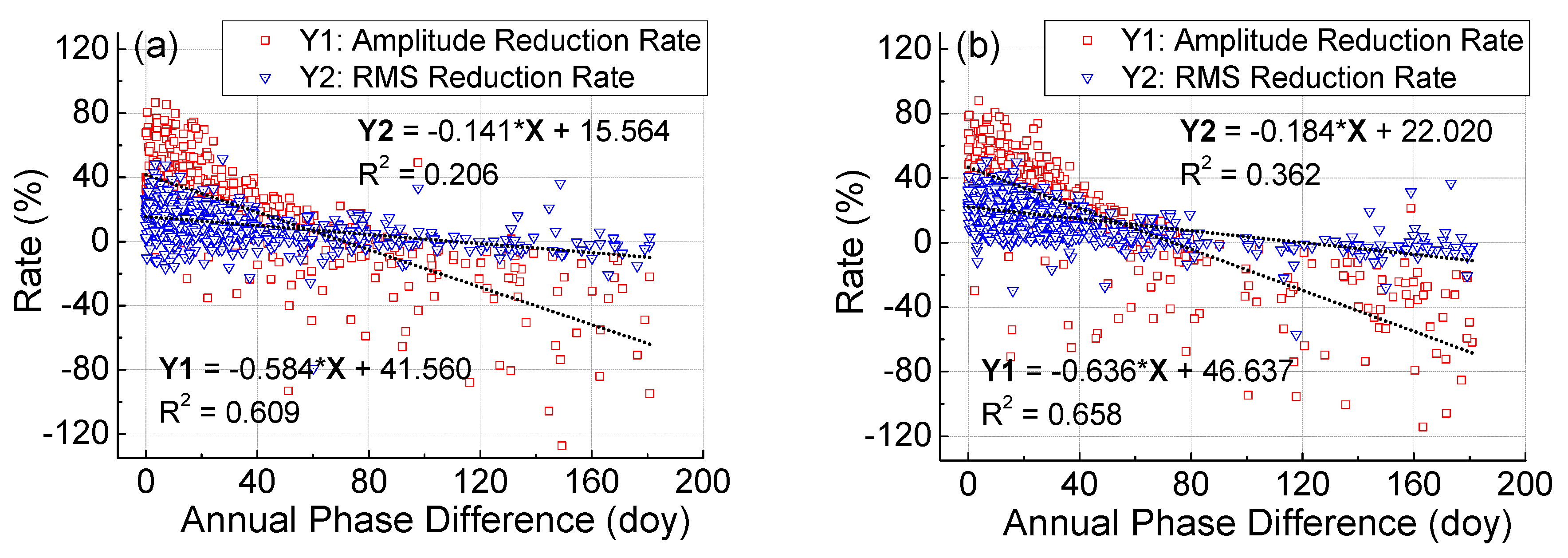
3.1. RMS Reduction Rate

After deducting the SUML displacement series of GFZ and EOST from the GPS height time series, RMS reduction rates are shown in Figure 2. It can be seen from Figure 2a,b that the RMS reduction rates at most stations (523) were positive, accounting for 82.6% of all 633 stations. It indicates that ELCs had a positive effect on correcting the nonlinear deformation of GPS height time series at most stations. As for the ELCs result of GFZ, the number of stations with RMS reduction rates between 0% and 10% was 211, accounting for 33.3% of the total stations. The average RMS reduction rate of all stations was 10.6%. From Figure 2c,d, more GPS stations (553) had decreased RMS values after ELCs of EOST, making up 87.4% of the total stations. The average RMS reduction rate of all stations was 15.4%.

From Figure 2a,c, the impact of ELCs on GPS height time series had obvious spatial distribution characteristics, and were similar to each other. Overall, the ELC effect in the middle and high latitudes was larger than that in low latitudes. In detail, GPS stations in northern North America, eastern Europe, northwestern Asia and Antarctica had a significant ELC effect where the RMS reduction rates were higher. In the southern United States, Central America, southern South America, central and southern Africa, the correction effect of environmental loadings was not obvious, even some stations with RMS increased.

According to the statistics of Figure 2a, the average RMS reduction rates of GPS stations in the low, middle and high latitude regions were 2.4%, 12.7% and 13.9%, respectively, while the counterparts for Figure 2c were 4.2%, 19.8% and 12.7%. In respect to RMS reduction rate, EOST loading series helped more than GFZ products in reducing the nonlinear variation at GPS stations. EOST showed a more concentrated distribution of RMS reduction rates than GFZ (Figure 2b vs. Figure 2d), with less extreme values. It is worth noting that there were gaps in the GPS height time series. In order to keep the same number of observations in the GPS and loading time series, the loading series (consecutive) was processed into nonconsecutive with the same epochs as the GPS series.

As observed from Figure 2a, the two African GPS stations located near equator, MBAR (Uganda, 30.7°E 0.6°S) and RCMN (Kenya, 36.9°E 1.2°S) had the lowest RMS reduction rates of −79.2% and −20.8%, respectively. MBAR is located on the shore of Lake Victoria, the largest African (and third largest worldwide) lake, and RCMN is nearby. However, these two stations did not show the same obvious negative ELC effect in EOST results as in the GFZ results, as shown in Figure 2a,c. The region is controlled by the equatorial low pressure, with annual rainfall and lake water being abundant. The hydro-climatic characteristics are complex and changeable, so different HYDL models in this small-sized area had large variations, as expressed in Figure 3a. In addition, for other GPS stations with negative RMS reduction rates, both GPS and environmental loading series contained obvious annual signals, and the large difference of their annual phases is likely to cause the GPS time series to be more scattered after ELCs. The reason will be further discussed in the next section.

This deviation between loading series from GFZ and EOST can also be represented at stations with positive RMS reduction rates. Observed from Figure 2a, two GPS stations near the equator, POVE (Brazil, 296.1°E 8.7°S) and KOUR (French Guiana, 307.2°E 5.3°N) had RMS reduction rates of 48.4% and 33.1%, respectively, significantly higher than other stations in the low latitude area. From the EOST results in Figure 2c, the counterparts of these two stations were 26.6% and 30.3%. These two stations are located in the Amazon rainforest and also controlled by the equatorial low-pressure zone. There are rich precipitation and lush vegetation that bring huge amounts of transpiration and evaporation. Compared with Lake Victoria, the Amazon rainforest is nearly 80 times larger in acreage, so it is more likely to be considered when establishing hydrological models; therefore, the real hydro-climatic characteristics can be acquired through these models, as shown in Figure 3b. The GPS height time series and loading series of GFZ and EOST at POVE tended to have similar annual amplitude and phases. After ELCs, RMS and the annual amplitude of the GPS-GFZ series greatly decreased. Although there was also an obvious decrease in RMS value for the GPS-EOST series, the residual seasonal terms were still obvious. Therefore, it was necessary to analyze the difference of the annual amplitude and phase with respect to GPS height time series, GFZ and EOST loading series.

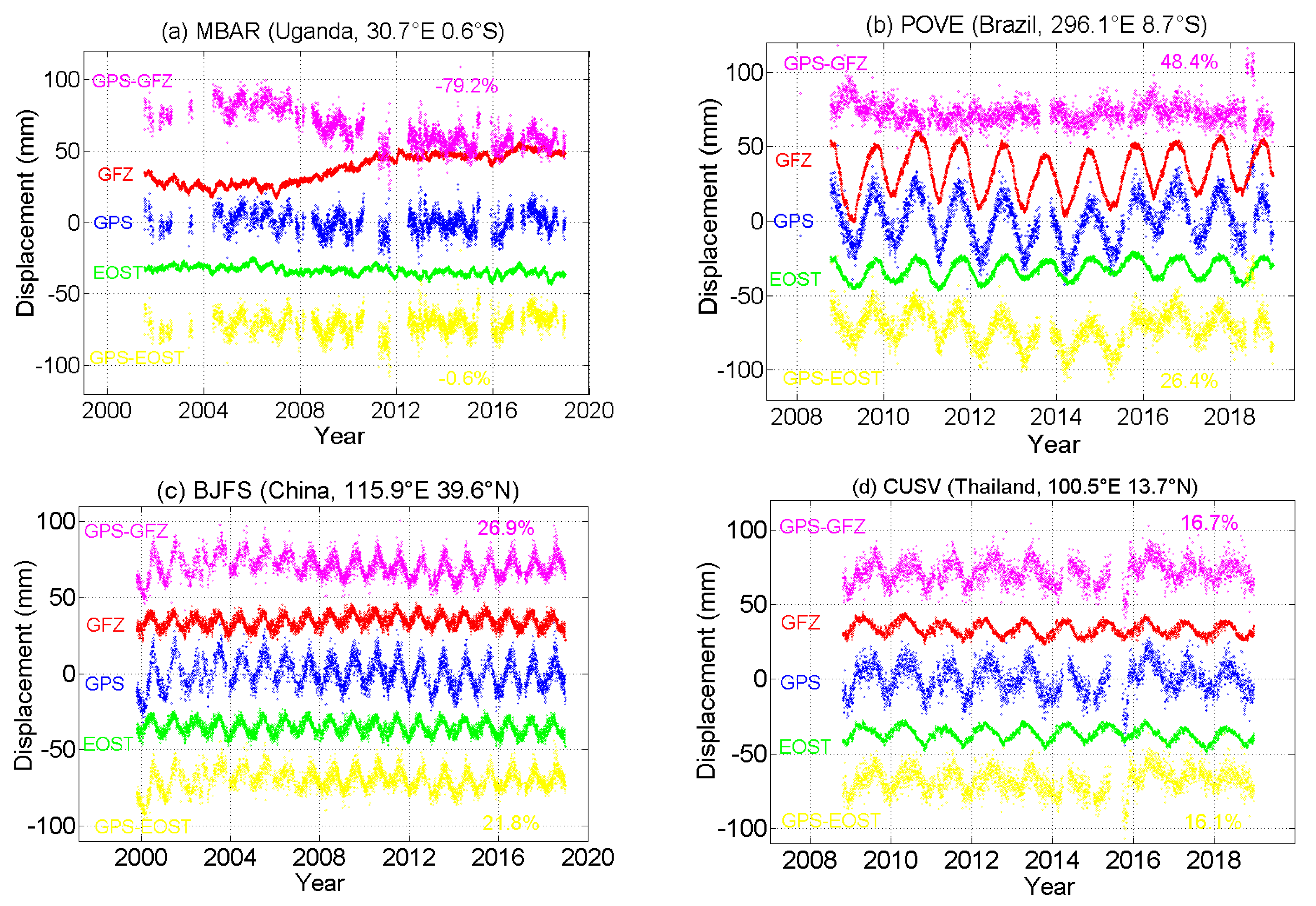
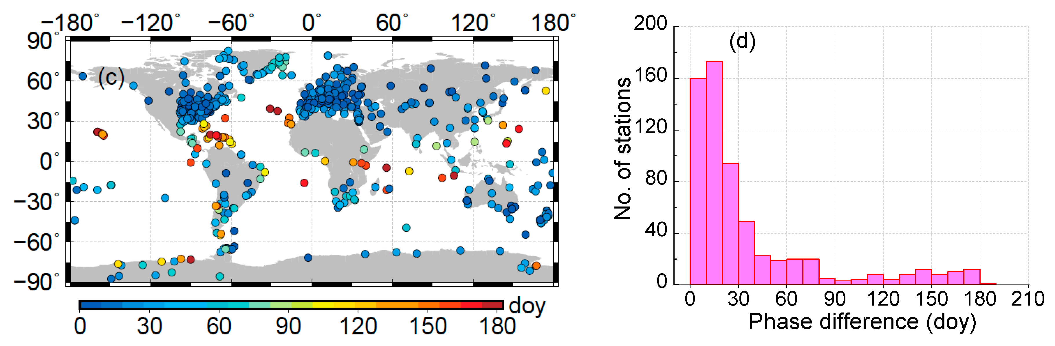
3.2. Annual Amplitude and Phase Change

Many studies have demonstrated that there are obvious periodic signals in GPS height time series, and among the signals of various frequencies, the amplitude of annual signal is the largest [43]. In order to study the influence of the loading series from GFZ and EOST on the characteristic changes of annual motion at global GPS stations, based on the WN+PL noise model, the annual amplitude and phase of GPS height time series were calculated before (Figure 4a,b) and after the ELC process (Figure 4g,h for GPS-GFZ; Figure 4i,j for GPS-EOST), and meanwhile the annual amplitude and phase of the loading series (Figure 4c,d for GFZ; Figure 4e,f for EOST).

As can be seen from Figure 4a, the GPS height time series contains strong annual signals with the maximal amplitude of ~20 mm (NOVM, Kazakhstan, 82.9°E 55.0°N). It means that the magnitude of nonlinear motion reaches centimeters at some GPS stations, so it is necessary to take into account the nonlinear variation at the GPS stations and the corresponding geophysical mechanisms when establishing the global terrestrial reference frame. For the spatial layout features of the annual amplitude, GPS stations in the northern hemisphere are generally larger than the southern hemisphere; Eurasia (especially its inland), larger than other continents; and land larger than islands. The average annual amplitude of all 633 stations was 7.2 mm.

The annual phase of the GPS height time series had more obvious global changes, as shown in Figure 4b. The annual phase of the GPS stations in the northern hemisphere mostly appeared during 180-270 days (expressed as day of year, DOY), that is, July to September. In the southern part of the Earth, annual phases were concentrated in 0-60 and 300-360 days, that is, November to February of next year. For these GPS stations, on the day of their annual phases, they were in the furthest place away from their initial positions and also the Earth’s center of figure. It can be explained that the annual phase of GPS height time series was directly related to the latitude of the subsolar point. In other words, when the subsolar point appeared in the northern hemisphere (spring equinox to summer solstice, then to autumn equinox), during this period (approximately 80-266 DOY), 93.9% of the GPS stations in the northern hemisphere responded by reaching their respective annual phases. Similarly, when the subsolar point wandered at the southern hemisphere (autumn equinox to winter solstice, then to spring equinox again), during this period (approximately 266 to 80 of next year), 62.6% of the GPS stations located here also responded. As the GPS stations in the Antarctic and Greenland somehow showed different phases to other regions in their respective hemispheres, the above two ratios would both increase after excluding the GPS stations in these two regions. The relationship between the annual phase of the GPS stations and the latitude of the subsolar point would be more obvious.

The annual amplitude and phase of the environmental loading series are shown in Figure 4c,d (for GFZ) and Figure 4e,f (for EOST). The comparison in Figure 4a,c,e shows that the annual amplitude of the environmental loading series was generally smaller than that of the GPS height time series. The average annual amplitudes of the GFZ and EOST loading series at 633 stations were 2.7 and 3.1 mm, respectively. Compared with the counterpart of the GPS series (7.2 mm), the environmental loading series of GFZ and EOST could explain about 38.4% and 43.3% of the GPS annual amplitude.

There were similar change features of spatial distribution among them, but meanwhile, an obvious difference existed. The annual amplitude of the GPS series in the northern hemisphere was generally larger than that in the southern hemisphere, while this feature seemed unapparent for GFZ and EOST loading series. The annual amplitude of the environmental loading series was larger in the inland of Eurasia and the Brazilian Plateau, such as POVE in Brazil, with the largest annual amplitude of 15.5 mm for the GFZ loading series.

The spatial distribution of the annual phase derived from the environmental loading series had more significant latitude-related and land-sea characteristics. For stations located on ocean islands, the annual amplitudes of GFZ and EOST were mostly distributed from DOY 330 to 120 of next year, that is, December to next April, and they also represented obvious latitude-related differences for stations situated on land. From the equator to 30°N, the annual phases of most stations appeared in DOY 30-120 (excluding island stations in the Caribbean Sea for GFZ), that is, February to April. From the equator to 30°S, annual phases of most stations appeared in 270-360, that is, October to December. From 30 to 60°N, most annual phases were distributed between 210 and 270 (August to September), while from 30 to 60°S, annual phases mostly emerged from 330 to 60 (December to next February). For high-latitude regions, the annual phases of the environmental loading series on the Greenland and Antarctica were concentrated near 210 and 360, standing for July and December, respectively. Compared with the GPS series, the annual phase of the environmental loading series had more obvious latitude-related distribution features.

After the ELC process, spatial distribution of the annual amplitude and phase are displayed in Figure 4g,h (for GPS-GFZ) and Figure 4i,j (for GPS-EOST). To ensure that parameter estimations before and after ELCs are not affected by stochastic models, the same WN+PL noise model was employed. Comparing Figure 4a with Figure 4g,i, the GPS annual amplitudes were decreased and its spatial features were also weakened. The average annual amplitude was 5.3 mm for GPS-GFZ and 4.9 mm for GPS-EOST after ELCs. Compared with the annual amplitude before ELCs (7.2 mm), the amplitude reduction rate was 26.6% for GFZ and 31.6% for EOST.

Particularly, stations NOVM and POVE had the two largest annual amplitudes of 19.5 and 18.1 mm before ELCs. While after ELCs, their annual amplitude decreased to 11.9 and 2.4 mm for GPS-GFZ series, and to 10.3 and 10.3 mm for GPS-EOST series. In GPS-GFZ series, the annual amplitude of TIXI (Russia, 128.9°E 71.6°N) was the largest (12.1 mm). Compared with its counterpart of 12.2 mm before ELCs, its annual amplitude reduction rate was only 0.9%. Even worse, the annual amplitude of 16.9% stations increased after GFZ correction, such as station WUHN (China, 114.4°E 30.5°N) increasing by 3.3 mm. Similarly in GPS-EOST series, the largest annual amplitude was 10.9 mm at station COVX (USA, 284.3°E 36.9°N), and the annual amplitude reduction rate was 9.3%. To facilitate further discussions, the annual amplitude and phase of the above 5 GPS stations are listed in

Table 1. Statistics of the annual amplitudes and phases at 5 GPS stations.

Stations	(°E)	(°N)	Country	Annual	GPS	GFZ	EOST	GPS-GFZ	GPS-EOST
NOVM	82.9	55.0	Kazakhstan	Ampli (mm)	19.5	7.5	9.1	11.9	10.3
				Phase (DOY)	211.8	217.0	214.4	208.2	209.3
POVE	296.1	−8.7	Brazil	Ampli	18.1	15.5	8.0	2.4	10.3
				Phase	280.9	277.5	287.4	35.2	274.0
TIXI	128.9	71.6	Russia	Ampli	12.2	0.6	4.9	12.1	7.4
				Phase	221.2	150.9	216.2	224.7	225.5
WUHN	114.4	30.5	China	Ampli	5.9	6.3	4.4	9.2	2.3
				Phase	186.1	92.9	174.8	231.7	213.1
COVX	284.3	36.9	USA	Ampli	12.0	0.6	1.1	11.5	10.9
				Phase	110.8	249.4	228.6	221.7	222.2

.

Comparing Figure 4b with Figure 4h,j, the GPS annual phase changed significantly after ELCs. The north–south difference of the annual phase was basically eliminated and it appeared at around DOY 230 for most stations. The percentage of stations with an annual phase between DOY 200 to 260 was 80.3% for GPS-GFZ series, and 78.4% for GPS-EOST series. In addition, the annual phase of the GPS stations located in southeastern Australia, New Zealand and nearby islands and the Antarctic were apparently different from other stations, most of which were distributed from DOY 300 to 60 of next year.

Andrei et al. [24] estimated the seasonal signals (including annual and semi-annual components) at station ABOA, a Finnish Antarctic station research station located in Dronning Maud Land, East Antarctic. Figure 5 shows the 32 Antarctic stations of this study and the station ABOA. Although ABOA was not included in this study, the station VESL is relatively near to it, so some comparisons could be made in

Table 2. Comparisons of the seasonal signals and spectral index between the GPS height time series at stations ABOA and VESL. The column “Mean” displays the average values of the 32 stations. (unit: mm).

	ABOA	VESL	Mean
Annual Ampli	2.43 ± 0.57	3.27 ± 0.59	3.05 ± 0.73
Semi-annual Ampli	2.14 ± 0.42	0.68 ± 0.34	1.45 ± 0.48
Annual Phase	23/24 August	21 July	14 May
Spectral Index	−0.9	−0.9	−1.0

. There were differences in the estimations of the annual and semi-annual amplitudes between ABOA and VESL. For station ABOA, the annual amplitude was a little larger than the semi-annual amplitude; while for VESL, the annual signal predominated in its annual motion. For all 32 stations, there were 7 stations with a difference of the annual amplitude and semi-annual amplitude smaller than 0.5 mm, so such differences were probably determined by the local geophysical effects. Overall, the average annual amplitude was 3.05 ± 0.73, nearly twice as much as the semi-annual amplitude. The spectral indexes of ABOA and VESL were nearly equal, which means that their height time series contained the same temporally correlated colored noise. The average index value for the total 32 stations was −1.0, so the GPS height time series at the Antarctic showed obvious flicker noise.

4. Discussions

Comparing the annual amplitude changes of five GPS stations before and after ELCs in Table 1, it can be seen that ELCs had a significant effect on the first two stations (NOVM and POVE). Their annual amplitude reduction rates are 39.2%, 86.5% after GFZ correction, and 47.3% and 47.2% for EOST correction, respectively. Loading series from GFZ and EOST both have a positive role in reducing the GPS annual amplitude. For station TIXI, the effect of GFZ correction is not obvious as its annual amplitude reduction rate is 0.9% only, while the effect of EOST correction is much better with the reduction rate of 39.2%. The difference exists because the EOST annual amplitude and phase is closer to the counterpart of the GPS series than GFZ. For station WUHN, the correction effect of GFZ and EOST loading series seems to have a larger difference, because the annual amplitude reduction rate is −56.1% for GFZ and 61.4% for EOST. Although GFZ annual amplitude (6.3 mm) is closer to the GPS annual amplitude (5.9 mm) than EOST (4.4 mm), its annual phase has a much larger difference with GPS than EOST. As a result, the GFZ loading series plays a negative role in reducing nonlinear motion at this station.

From the above discussions, it is obvious to conclude that ELCs perform effectively at some stations where GPS series and loading series not only have similar annual amplitudes but also similar annual phases. Therefore, after the ELC process, the GPS series contains much less fluctuations, so the nonlinear motion becomes significantly weakened. For station NOVM, although its annual amplitudes of GPS series and loading series are quite different, the annual phase difference is only in a range of a few days, so a good ELC effect can also be obtained. On the other hand, ELCs will result in poor effects at stations where there is a large difference of annual phase between GPS series and loading series, despite a small difference of annual amplitude between them. The peaks of the two series cannot be eliminated in the differencing process, leading to the nonlinear motion in the GPS series increasing, such as the GFZ effect at station WUHN.

In order to visually show the ELC effect at the total number of GPS stations, the annual amplitude reduction rate of GPS series and its histogram were obtained, as shown in Figure 6. The annual amplitude reduction rates at most GPS stations are positive, accounting for 83.1% of total stations for GFZ correction and 82.8% for EOST correction. It indicates that environmental loadings have a positive effect on the annual variations at most GPS stations. The average annual amplitude reduction rate of all stations is 21.1% for GFZ and 23.9% for EOST. Specifically, the annual amplitude reduction rate of GPS stations located in Eurasia, Australia, northern North America and central South America is more obvious, while for stations in Central America, the Caribbean Sea and some marine islands, the annual amplitude reduction rates are comparatively small.

In order to investigate the relationship between the ELC effect and annual phase difference, the absolute phase differences between the GPS series and GFZ, EOST loading series were calculated. The spatial distribution and histograms of the absolute phase difference are shown in Figure 7 (|GPS-GFZ| for Figure 7a,b; |GPS-EOST| for Figure 7c,d). The number of GPS stations with a phase difference of 0-30 days (one month) is 410 for GFZ, and 427 for EOST, accounting for 64.8% and 67.5% of all stations, respectively. Comparing Figure 6 and Figure 7, the annual phase differences and the annual amplitude reduction rates at the GPS stations have a comparatively consistent spatial distribution, similarly showing that the annual phase differences in the GPS stations located in Central America and some ocean islands are obviously different from stations in other regions.

Figure 8 illustrates the linear relationship between the annual phase difference (assumed as independent variable X), annual amplitude reduction rate (dependent variable Y1) and RMS reduction rate (dependent variable Y2). It is apparent that there is a strong linear relationship between annual phase difference X, annual amplitude reduction rate Y1 and RMS reduction rate Y2, indicating that the annual phase difference directly affects the reduction rate of the annual amplitude and RMS.

According to the linear fitting results in Figure 8a (GPS vs. GFZ), when the annual phase difference is zero, the reduction rates of annual amplitude and RMS will be the largest, which are 41.6% and 15.6%, respectively. The two ratios are larger in the fitting results of Figure 8b (GPS vs. EOST), which means EOST loading series are possibly more helpful in reducing the nonlinear variations in the GPS time series. In addition, the goodness of fit between X and Y1 is greater than that between X and Y2, indicating that the linear relationship between the annual phase difference and the annual amplitude reduction rate is stronger.

5. Conclusions

This paper analyzes the characteristic changes of 20 year GPS height time series of global 633 stations before and after the environmental loading corrections of GFZ and EOST products, including the reduction rate of RMS, annual amplitude and annual phase difference. Some conclusions were drawn as follows:

Environmental loading corrections have a positive effect on the reduction in the nonlinear motion in GPS height time series of the global GPS stations. RMS reduction rate is positive at 82.6% of stations for GFZ correction and 87.4% for EOST correction, and the average value of all stations is 10.6% and 15.4%, respectively. RMS reduction rate shows an obvious latitude correlation that the ELC effect in the middle and high latitude performs better than in the low latitude.

As for the GPS height time series, the annual amplitudes in the northern hemisphere are generally larger than that in the southern hemisphere; Eurasia (especially its inland), larger than other continents; and land larger than islands. The average annual amplitude of all GPS stations is 7.2 mm. The global layout characteristics of the annual phase are obvious. Most of the annual phases in the northern hemisphere appear from July to September, while in the southern hemisphere, they are concentrated from December to next February. The annual phase of the GPS height time series is affected by the latitude of the subsolar point.

As for the environmental loading series of GFZ and EOST, their average annual amplitude is 2.7 and 3.1 mm, which explains the ~40% annual amplitude of the GPS height time series. The annual amplitude derived from the environmental loading series is generally smaller than that from the GPS height time series, and they have similar characteristics of spatial distribution. Compared with GPS height time series, the annual phase of environmental loading series shows a more obvious latitude correlation.

After ELCs, the annual amplitudes of most GPS height series are decreased, and their spatial features are also weakened. The average annual amplitude is 5.3 mm for GPS-GFZ and 4.9 mm for GPS-EOST after ELCs. Compared with the annual amplitude before ELCs (7.2 mm), the amplitude reduction rate is ~30%. The annual phases of GPS height time series also change significantly. They are distributed around 230 days in most stations, and are distributed between 200~260 days for ~80% stations.

The effect of ELCs varies greatly among global GPS stations. The largest annual amplitude reduction rate can reach about 87%, while for some stations, the nonlinear motion increases significantly after ELCs. The difference between the annual amplitude and phase of GPS height time series and environmental loading series can be an immediate reason for the unevenness of ELC effects, and the annual phase difference has a greater influence.

According to the fitting results of the RMS reduction rate, annual amplitude reduction rate and annual phase difference, the linear relationship between the annual phase difference and the annual amplitude reduction rate is stronger. Meanwhile, EOST loading series are possibly more helpful in reducing the nonlinear variations in GPS time series.

References

1. Blewitt, G.; Lavallee, D.; Clarke, P.; Nurutdinov, K. A new global mode of Earth deformation: Seasonal cycle detected. Science 2001, 294, 2342–2345. [Google Scholar] [CrossRef] [PubMed] [Green Version]
2. Wang, M.; Shen, Z.; Dong, D. Effects of non-tectonic crustal deformation on continuous GPS position time series and correction to them. Chin. J. Geophys. 2005, 48, 1045–1052. [Google Scholar] [CrossRef]
3. Ray, J.; Altamimi, Z.; Collilieux, X.; van Dam, T. Anomalous harmonics in the spectra of GPS position estimates. GPS Solut. 2008, 12, 55–64. [Google Scholar] [CrossRef]
4. Klos, A.; Bos, M.; Bogusz, J. Detecting time-varying seasonal signal in GPS position time series with different noise levels. GPS Solut. 2018, 22, 21. [Google Scholar] [CrossRef] [Green Version]
5. Klos, A.; Olivares, G.; Teferle, F.; Hunegnaw, A.; Bogusz, J. On the combined effect of periodic signals and colored noise on velocity uncertainties. GPS Solut. 2018, 22, 1–13. [Google Scholar] [CrossRef] [Green Version]
6. Williams, S.; Bock, Y.; Fang, P.; Jamason, P.; Nikolaidis, R.; Prawirodirdjo, L.; Miller, M.; Johnson, D. Error analysis of continuous GPS position time series. J. Geophys. Res. Solid Earth 2004, 109, B03412. [Google Scholar] [CrossRef] [Green Version]
7. Beavan, R.J. Noise properties of continuous GPS data from concrete pillar geodetic monuments in New Zealand, and comparison with data from deep drilled braced monuments. J. Geophys. Res. Solid Earth 2005, 110, B8. [Google Scholar] [CrossRef]
8. Langbein, J. Noise in GPS displacement measurements from Southern California and Southern Nevada. J. Geophys. Res. Solid Earth 2008, 113, B05405. [Google Scholar] [CrossRef]
9. Yuan, L.; Ding, X.; Chen, W.; Guo, Z.; Chen, S.; Hong, B.; Zhou, J. Characteristics of daily position time series from the Hong Kong GPS fiducial network. Chin. J. Geophys. 2008, 51, 1372–1384. [Google Scholar] [CrossRef]
10. Dong, D.; Fang, P.; Bock, Y.; Cheng, M.K.; Miyazaki, S. Anatomy of apparent seasonal variations from GPS-derived site position time series. J. Geophys. Res. Solid Earth 2002, 107, ETG 9-1–ETG 9-16. [Google Scholar] [CrossRef] [Green Version]
11. Márquez-Azúa, B.; DeMets, C. Crustal velocity field of Mexico from continuous GPS measurements, 1993 to June 2001: Implications for the neotectonics of Mexico. J. Geophys. Res. Solid Earth 2003, 108, B9. [Google Scholar] [CrossRef]
12. Tian, Y.; Shen, Z. Extracting the regional common-mode component of GPS station position time series from dense continuous network. J. Geophys. Res. Solid Earth 2016, 121, 1080–1096. [Google Scholar] [CrossRef]
13. Ma, C.; Li, F.; Zhang, S.; Lei, J.; E, D.; Hao, W.; Zhang, Q. The coordinate time series analysis of continuous GPS stations in the Antarctic Peninsula with consideration of common mode error. Chin. J. Geophys. 2016, 59, 2783–2795. [Google Scholar] [CrossRef]
14. Ming, F.; Yang, Y.; Zeng, A.; Zhao, B. Spatiotemporal filtering for regional GPS network in China using independent component analysis. J. Geod. 2017, 91, 419–440. [Google Scholar] [CrossRef]
15. van Dam, T.; Blewitt, G.; Heflin, M. Atmospheric pressure loading effects on Global Positioning System coordinate determinations. J. Geophys. Res. Solid Earth 1994, 99, 23939–23950. [Google Scholar] [CrossRef]
16. van Dam, T.; Wahr, J.; Milly, P.; Shmakin, A.; Blewitt, G.; Lavallée, D.; Larson, K. Crustal displacements due to continental water loading. Geophys. Res. Lett. 2001, 28, 651–654. [Google Scholar] [CrossRef] [Green Version]
17. van Dam, T.; Altamimi, Z.; Collilieux, X.; Ray, J. Topographically induced height errors in predicted atmospheric loading effects. J. Geophys. Res. Atmos. 2010, 115, B07415. [Google Scholar] [CrossRef]
18. Jiang, W.; Li, Z.; van Dam, T.; Ding, W. Comparative analysis of different environmental loading methods and their impacts on the GPS height time series. J. Geod. 2013, 87, 687–703. [Google Scholar] [CrossRef]
19. Jiang, W.; Li, Z.; Liu, H.; Zhao, Q. Cause analysis of the non-linear variation of the IGS reference station coordinate time series inside China. Chin. J. Geophys. 2013, 56, 2228–2237. [Google Scholar] [CrossRef]
20. Gu, Y.; Yuan, L.; Fan, D.; You, W.; Su, Y. Seasonal crustal vertical deformation induced by environmental mass loading in mainland China derived from GPS, GRACE and surface loading models. Adv. Space Res. 2017, 59, 88–102. [Google Scholar] [CrossRef]
21. Chanard, K.; Fleitout, L.; Calais, E.; Rebischung, P.; Avouac, J. Toward a global horizontal and vertical elastic load deforma-tion model derived from GRACE and GNSS station position time series. J. Geophys. Res. Solid Earth 2018, 123, 3225–3237. [Google Scholar] [CrossRef]
22. Yuan, P.; Li, Z.; Jiang, W.; Ma, Y.; Chen, W.; Sneeuw, N. Influences of environmental loading corrections on the nonlinear variations and velocity uncertainties for the reprocessed global positioning system height time series of the crustal movement observation network of China. Remote Sens. 2018, 10, 958. [Google Scholar] [CrossRef] [Green Version]
23. Klos, A.; Gruszczynska, M.; Bos, M.; Boy, J.; Bogusz, J. Estimates of vertical velocity errors for IGS ITRF2014 stations by applying the improved singular spectrum analysis method and environmental loading models. Pure Appl. Geophys. 2018, 175, 1823–1840. [Google Scholar] [CrossRef]
24. Andrei, C.; Lahtinen, S.; Nordman, M.; Näränen, J.; Koivula, H.; Poutanen, M.; Hyyppä, J. GPS time series analysis from aboa the finnish antarctic research station. Remote Sens. 2018, 10, 1937. [Google Scholar] [CrossRef] [Green Version]
25. Li, Z.; Chen, W.; van Dam, T.; Rebischung, P.; Altamimi, Z. Comparative analysis of different atmospheric surface pressure models and their impacts on daily ITRF2014 GNSS residual time series. J. Geod. 2020, 94, 42–61. [Google Scholar] [CrossRef]
26. Li, C.; Huang, S.; Chen, Q.; Dam, T.; Fok, H.; Zhao, Q.; Wu, W.; Wang, X. Quantitative Evaluation of Environmental Loading Induced Displacement Products for Correcting GNSS Time Series in CMONOC. Remote Sens. 2020, 12, 594. [Google Scholar] [CrossRef] [Green Version]
27. Santamaría-Gómez, A.; Bouin, M.; Collilieux, X.; Wöppelmann, G. Correlated errors in GPS position time series: Implications for velocity estimates. J. Geophys. Res. Solid Earth 2011, 116, B01405. [Google Scholar] [CrossRef]
28. Jiang, W.; Zhou, X. Effect of the span of Australian GPS coordinate time series in establishing an optimal noise model. Sci. China Earth Sci. 2014, 44, 2461–2478. [Google Scholar] [CrossRef]
29. Farrell, W. Deformation of the Earth by surface loads. Rev. Geophys. 1972, 10, 761–797. [Google Scholar] [CrossRef]
30. van Dam, T.; Wahr, J. Displacements of the Earth’s surface due to atmospheric loading: Effects on gravity and baseline measurements. J. Geophys. Res. Solid Earth 1987, 92, 1281–1286. [Google Scholar] [CrossRef]
31. ESMGFZ Product Repository. Available online: http://rz-vm115.gfz-potsdam.de:8080/repository (accessed on 29 August 2020).
32. Dill, R.; Dobslaw, H. Numerical simulations of global scale high-resolution hydrological crustal deformations. J. Geophys. Res. Solid Earth 2013, 118, 5008–5017. [Google Scholar] [CrossRef]
33. Mémin, A.; Boy, J.; Santamaría-Gómez, A. Correcting GPS measurements for non-tidal loading. GPS Solut. 2020, 24, 45. [Google Scholar] [CrossRef]
34. Marsland, S.; Haak, H.; Jungclaus, J.; Latif, M.; Roske, F. The Max-Planck-Institute global ocean/sea-ice model with orthogonal curvilinear coordinates. Ocean Model. 2003, 5, 91–127. [Google Scholar] [CrossRef] [Green Version]
35. Dill, R. Hydrological model LSDM for operational Earth rotation and gravity field variations. Sci. Tech. Rep. 2008. [Google Scholar] [CrossRef]
36. Berrisford, P.; Dee, D.; Poli, P.; Brugge, R.; Fielding, K.; Fuentes, M.; Kallberg, P.; Kobayashi, S.; Uppala, S.; Simmons, A. ERA Report Series: The ERA-Interim Archive Version 2.0; European Centre for Medium Range Weather Forecasts: Shinfield Park, UK, 2011; pp. 1–27. [Google Scholar]
37. Gelaro, R.; McCarty, W.; Suárez, M.J.; Todling, R.; Molod, A.; Takacs, L.; Randles, C.A.; Darmenov, A.; Bosilovich, M.G.; Reichle, R.; et al. The modern-era retrospective analysis for research and applications, version 2 (MERRA-2). J. Clim. 2017, 30, 5419–5454. [Google Scholar] [CrossRef] [PubMed]
38. Menemenlis, D.; Campin, J.; Heimbach, P.; Hill, C.; Lee, T.; Nguyen, A.; Schodlok, M.; Zhang, H. ECCO2: High resolution global ocean and sea ice data synthesis. Mercat. Ocean Q. Newsl. 2008, 31, 13–21. [Google Scholar]
39. Bevis, M.; Brown, A. Trajectory models and reference frames for crustal motion geodesy. J. Geod. 2014, 88, 283–311. [Google Scholar] [CrossRef] [Green Version]
40. Bos, M.; Fernandes, R. Hector User Manual Version 1.6. 2016. Available online: http://segal.ubi.pt/hector/manual_1.7.2.pdf (accessed on 29 August 2020).
41. Williams, S. CATS: GPS coordinate time series analysis software. GPS Solut. 2008, 12, 147–153. [Google Scholar] [CrossRef]
42. Bos, M.; Fernandes, R.; Williams, S.; Bastos, L. Fast error analysis of continuous GNSS observations with missing data. J. Geod. 2013, 87, 351–360. [Google Scholar] [CrossRef] [Green Version]
43. Freymueller, J. Seasonal position variations and regional reference frame realization. In GRF2006 Symposium Proceedings, International Association of Geodesy Symposia; Bosch, W., Drewes, H., Eds.; Springer: Berlin, Germany, 2009; Volume 134, pp. 191–196. [Google Scholar] [CrossRef]
Figure 1. Layout of 633 global GPS stations and their effective time spans in 20 years (1999~2018).
Remotesensing 12 02822 g001
Figure 2. Root mean square (RMS) reduction rates of the 633 global Global Positioning System (GPS) stations after environmental loading corrections (ELCs) and their histograms. Panels (a,b) show the ELC effect by deducting GFZ loading series, while panels (c,d) illustrate the effect of EOST loading series. For clear comparison, panel (d) keeps the same range of abscissa and ordinate axes as panel (b).
Remotesensing 12 02822 g002
Figure 3. Comparison of ELCs effect in four GPS stations (a) MBAR, (b) POVE, (c) BJFS and (d) CUSV. Scatters in blue, red and green represent GPS height series, environmental loading series from GFZ and EOST. Scatters in magenta and yellow are GPS residual series after removing loading series from GFZ and EOST. For clearance, GFZ and EOST series were moved upward and downward 35 mm. GPS-GFZ and GPS-EOST series were moved 70 mm.
Remotesensing 12 02822 g003
Figure 4. Spatial distribution of the annual amplitude (left panels) and phase (right panels) derived from 5 kinds of series (a,b) GPS, (c,d) GFZ, (e,f) EOST, (g,h) GPS-GFZ, (i,j) GPS-EOST at global GPS stations. In order to clearly show the change of distribution features, the scales of the annual amplitude (left panels) are different.
Remotesensing 12 02822 g004aRemotesensing 12 02822 g004b
Figure 5. Spatial layout of the Antarctic GPS stations. The 32 blue triangles represent the GPS stations of this study, and the red dot denotes the ABOA station in Andrei et al.
Remotesensing 12 02822 g005
Figure 6. Layout of the annual amplitude reduction rate of GPS height time series after GFZ and EOST loading corrections (panels (a,c)) and their corresponding histograms (panels (b,d)).
Remotesensing 12 02822 g006
Figure 7. Layout of the absolute differences between the annual phases derived from GPS height time series and environmental loading series of (a) GFZ and (c) EOST, and their corresponding histograms (b,d).
Remotesensing 12 02822 g007aRemotesensing 12 02822 g007b
Figure 8. Linear fitting of annual phase differences (X) with reduction rates of annual amplitude (Y1) and RMS (Y2). Panel (a) shows GPS vs. GFZ results, and panel (b) shows GPS vs. EOST results.
Remotesensing 12 02822 g008