Performances of Polarization-Retrieve Imaging in Stratified Dispersion Media


Abstract
:
1. Introduction
2. Theory and Method
2.1. PR Method
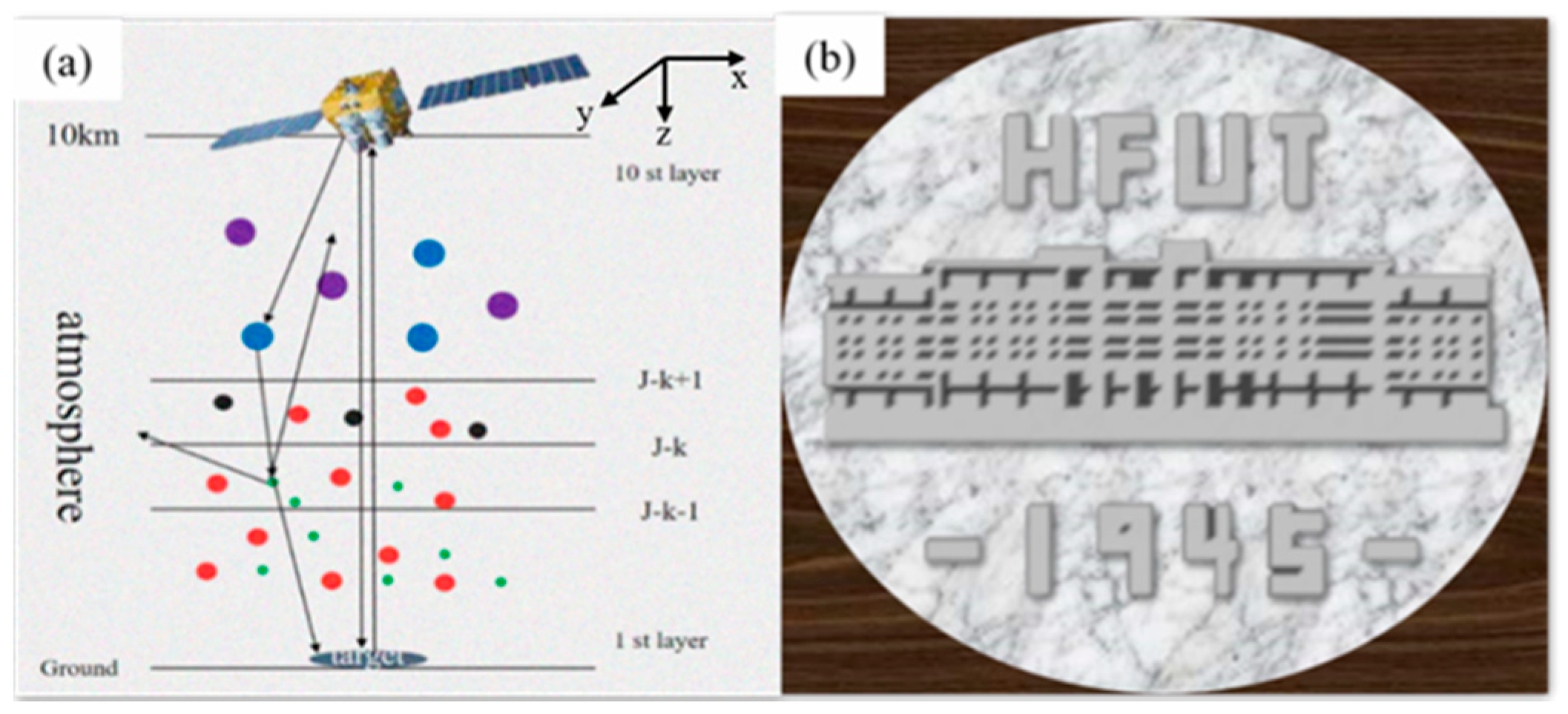
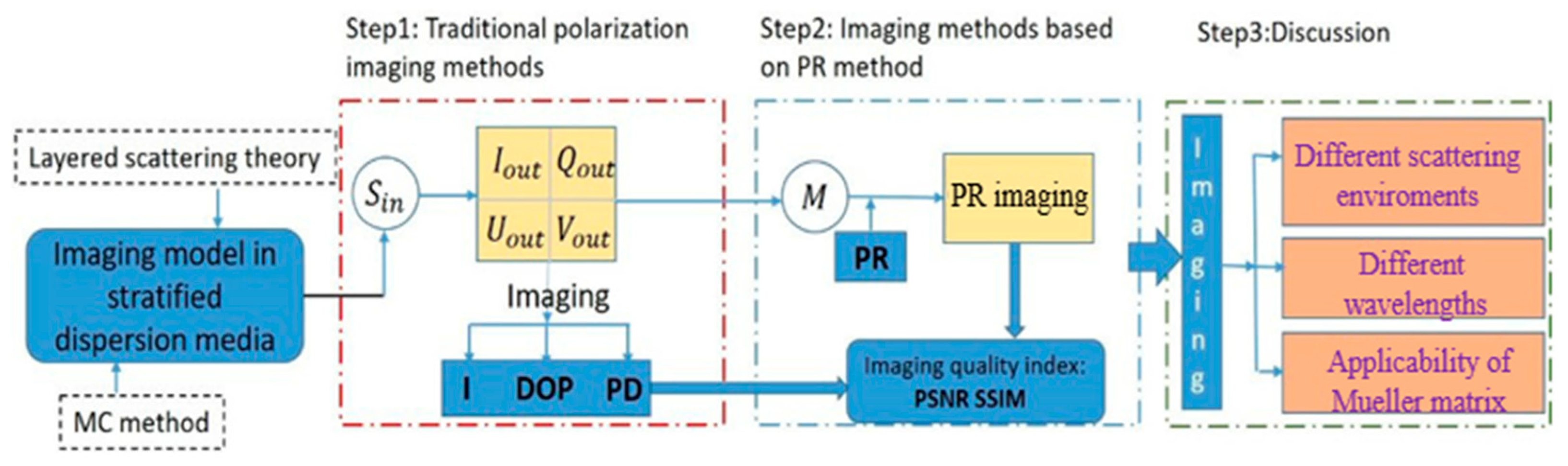
2.2. Simulation Method
3. Results and Discussions
4. Conclusions
Author Contributions
Funding
Conflicts of Interest
References
- Chiang, J.; Chen, Y.-C. Underwater Image Enhancement by Wavelength Compensation and Dehazing. IEEE Trans. Image Process. 2011, 21, 1756–1769. [Google Scholar] [CrossRef] [PubMed]
- Gu, Y.; Carrizo, C.; Gilerson, A.; Brady, P.C.; Cummings, M.E.; Twardowski, M.S.; Sullivan, J.M.; Ibrahim, A.; Kattawar, G.W. Polarimetric imaging and retrieval of target polarization characteristics in underwater environment. Appl. Opt. 2016, 55, 626–637. [Google Scholar] [CrossRef]
- He, Y.; Yang, B.; Lin, H.; Zhang, J. Modeling Polarized Reflectance of Natural Land Surfaces Using Generalized RegreSSIon Neural Networks. Remote Sens. 2020, 12, 248. [Google Scholar] [CrossRef] [Green Version]
- Fang, S.; Xia, X.; Xing, H.; Chen, C.; Huo, X. Image dehazing using polarization effects of objects and airlight. Opt. Express 2014, 22, 19523–19537. [Google Scholar] [CrossRef] [PubMed]
- Yeh, C.-H.; Kang, L.-W.; Lee, M.-S.; Lin, C.-Y. Haze effect removal from image via haze density estimation in optical model. Opt. Express 2013, 21, 27127–27141. [Google Scholar] [CrossRef] [PubMed]
- Zhang, W.; Liang, J.; Ren, L.; Ju, H.; Qu, E.; Bai, Z.; Tang, Y.; Wu, Z. Real-time image haze removal using an aperture-division polarimetric camera. Appl. Opt. 2017, 56, 942. [Google Scholar] [CrossRef]
- Sankaran, V.; Walsh, J.T.; Duncan, J.M. Polarized light propagation through tissue phantoms containing densely packed scatterers. Opt. Lett. 2000, 25, 239–241. [Google Scholar] [CrossRef]
- Shen, F.; Zhang, B.; Guo, K.; Yin, Z.; Guo, Z. The Depolarization Performances of the Polarized Light in Different Scattering Media Systems. IEEE Photon J. 2018, 10, 1–12. [Google Scholar] [CrossRef]
- Dechesne, C.; Lefèvre, S.; Vadaine, R.; Hajduch, G.; Fablet, R. Ship Identification and Characterization in Sentinel-1 SAR Images with Multi-Task Deep Learnin. Remote Sens. 2019, 11, 2997. [Google Scholar] [CrossRef] [Green Version]
- Zhai, A.; Wen, X.; Xu, H.; Yuan, L.; Meng, Q. Multi-Layer Model Based on Multi-Scale and Multi-Feature Fusion for SAR Images. Remote Sens. 2017, 9, 1085. [Google Scholar] [CrossRef] [Green Version]
- Hayashi, Y.; Tachibana, K. Mie-Scattering Ellipsometry for Analysis of Particle Behaviors in ProceSSIng Plasmas. Jpn. J. Appl. Phys. 1994, 33, L476–L478. [Google Scholar] [CrossRef]
- Groth, S.; Greiner, F.; Tadsen, B.; Piel, A. Kinetic Mie ellipsometry to determine the time-resolved particle growth in nanodusty plasmas. J. Phys. D Appl. Phys. 2015, 48, 465203. [Google Scholar] [CrossRef]
- Antonelli, M.-R.; Pierangelo, A.; Novikova, T.; Validire, P.; Benali, A.; Gayet, B.; De Martino, A. Impulse response solution to the three-dimensional vector radiative transfer equation in atmosphere-ocean systems. I. Monte Carlo method. Opt. Express 2010, 18, 10200–10208. [Google Scholar] [CrossRef] [PubMed]
- Kirchschlager, F.; Wolf, S.; Greiner, F.; Groth, S.; Labdon, A. In-situanalysis of optically thick nanoparticle clouds. Appl. Phys. Lett. 2017, 110, 173106. [Google Scholar] [CrossRef] [Green Version]
- Liu, F.; Wei, Y.; Han, P.; Yang, K.; Bai, L.; Shao, X. Polarization-based exploration for clear underwater vision in natural illumination. Opt. Express 2019, 27, 3629–3641. [Google Scholar] [CrossRef] [PubMed]
- Chen, Z.; Zhang, D.; Xu, Y.; Wang, C.; Yuan, B. Research of Polarized Image Defogging Technique Based on Dark Channel Priori and Guided Filtering. Procedia Comput. Sci. 2018, 131, 289–294. [Google Scholar] [CrossRef]
- Tyo, J.S.; Rowe, M.P.; Pugh, E.N.; Engheta, N. Target detection in optically scattering media by polarization-difference imaging. Appl. Opt. 1996, 35, 1855–1870. [Google Scholar] [CrossRef]
- Schechner, Y.Y.; Narasimhan, S.G.; Nayar, S.K. Instant dehazing of images using polarization. In Proceedings of the 2001 IEEE Computer Society Conference on Computer Vision and Pattern Recognition CVPR 2001 CVPR-01 2005, Kauai, HI, USA, 8–14 December 2001. [Google Scholar] [CrossRef] [Green Version]
- Schechner, Y.; Karpel, N. Recovery of Underwater Visibility and Structure by Polarization Analysis. IEEE J. Ocean Eng. 2005, 30, 570–587. [Google Scholar] [CrossRef] [Green Version]
- Dubreuil, M.; Delrot, P.; Leonard, I.; Alfalou, A.; Brosseau, C.; Dogariu, A. Exploring underwater target detection by imaging polarimetry and correlation techniques. Appl. Opt. 2013, 52, 997–1005. [Google Scholar] [CrossRef]
- Huang, B.; Liu, T.; Hu, H.; Han, J.; Yu, M. Underwater image recovery considering polarization effects of objects. Opt. Express 2016, 24, 9826–9838. [Google Scholar] [CrossRef]
- Liang, J.; Ren, L.-Y.; Ju, H.-J.; Qu, E.-S.; Wang, Y.-L. Visibility enhancement of hazy images based on a universal polarimetric imaging method. J. Appl. Phys. 2014, 116, 173107. [Google Scholar] [CrossRef]
- Liang, J.; Ren, L.; Ju, H.; Zhang, W.; Qu, E. Polarimetric dehazing method for dense haze removal based on distribution analysis of angle of polarization. Opt. Express 2015, 23, 26146–26157. [Google Scholar] [CrossRef] [PubMed]
- Liang, J.; Zhang, W.; Ren, L.; Ju, H.; Qu, E. Polarimetric dehazing method for visibility improvement based on visible and infrared image fusion. Appl. Opt. 2016, 55, 8221. [Google Scholar] [CrossRef] [PubMed]
- Hu, H.; Zhao, L.; Li, X.; Wang, H.; Liu, T. Underwater Image Recovery under the Nonuniform Optical Field Based on Polarimetric Imaging. IEEE Photon J. 2018, 10, 1–9. [Google Scholar] [CrossRef]
- Marchuk, G.I.; Mikhailov, G.A.; Nazaraliev, M.A.; Darbinjan, R.A.; Kargin, B.A.; Elepov, B.S. The Monte Carlo Methods in Atmospheric Optics. In X-ray Microsc; Springer: Berlin/Heidelberg, Germany, 1980. [Google Scholar]
- Ramella-Roman, J.C.; Prahl, S.A.; Jacques, S.L. Three Monte Carlo programs of polarized light transport into scattering media: Part I. Opt. Express 2005, 13, 4420–4438. [Google Scholar] [CrossRef]
- Hu, T.; Shen, F.; Wang, K.; Guo, K.; Liu, X.; Wang, F.; Peng, Z.; Cui, Y.; Sun, R.; Ding, Z.; et al. Broad-Band TransmiSSIon Characteristics of Polarizations in Foggy Environments. Atmosphere 2019, 10, 342. [Google Scholar] [CrossRef] [Green Version]
- Shen, F.; Zhang, M.; Guo, K.; Zhou, H.; Peng, Z.; Cui, Y.; Wang, F.; Gao, J.; Guo, Z. The depolarization performances of scattering systems based on the Indices of Polarimetric Purity (IPPs). Opt. Express 2019, 27, 28337–28349. [Google Scholar] [CrossRef]
- Shen, F.; Wang, K.; Tao, Q.; Xu, X.; Wu, R.; Guo, K.; Zhou, H.; Yin, Z.; Guo, Z. Polarization imaging performances based on different retrieving Mueller matrixes. Optik 2018, 153, 50–57. [Google Scholar] [CrossRef]
- Wang, C.; Gao, J.; Yao, T.; Wang, L.; Sun, Y.; Xie, Z.; Guo, Z. Acquiring reflective polarization from arbitrary multi-layer surface based on Monte Carlo simulation. Opt. Express 2016, 24, 9397–9411. [Google Scholar] [CrossRef]
- Xu, Q.; Guo, Z.; Tao, Q.; Jiao, W.; Qu, S.; Gao, J. A novel method of retrieving the polarization qubits after being transmitted in turbid media. J. Opt. 2015, 17, 35606. [Google Scholar] [CrossRef]
- Zhongyi, G.; Wang, X.; Li, D.; Wang, P.; Zhang, N.; Hu, T.; Zhang, M.; Gao, J. Advances on theory and application of polarization information propagation(Invited). Infrared Laser Eng. 2020, 49, 20201013. (In Chinese) [Google Scholar] [CrossRef]
- Xu, Q.; Guo, Z.; Tao, Q.; Jiao, W.; Qu, S.; Gao, J. Multi-spectral characteristics of polarization retrieve in various atmospheric conditions. Opt. Commun. 2015, 339, 167–170. [Google Scholar] [CrossRef]
- Tao, Q.; Guo, Z.; Xu, Q.; Jiao, W.; Wang, X.; Qu, S.; Gao, J. Retrieving the polarization information for satellite-to-ground light communication. J. Opt. 2015, 17, 85701. [Google Scholar] [CrossRef]
- Zhai, P.-W.; Kattawar, G.W.; Yang, P. Impulse response solution to the three-dimensional vector radiative transfer equation in atmosphere-ocean systems. I. Monte Carlo method. Appl. Opt. 2008, 47, 1037–1047. [Google Scholar] [CrossRef]
- Xu, Q.; Guo, Z.; Tao, Q.; Jiao, W.; Wang, X.; Qu, S.; Gao, J. Transmitting characteristics of polarization information under seawater. Appl. Opt. 2015, 54, 6584–6588. [Google Scholar] [CrossRef]
- Tao, Q.; Sun, Y.; Shen, F.; Xu, Q.; Gao, J.; Guo, Z. Active imaging with the aids of polarization retrieve in turbid media system. Opt. Commun. 2016, 359, 405–410. [Google Scholar] [CrossRef]
- Lawless, R.; Xie, Y.; Yang, P.; Kattawar, G.W.; Laszlo, I. Polarization and effective Mueller matrix for multiple scattering of light by nonspherical ice crystals. Opt. Express 2006, 14, 6381–6393. [Google Scholar] [CrossRef]
- Shao, H.; He, Y.; Li, W.; Ma, H. Polarization-degree imaging contrast in turbid media: A quantitative study. Appl. Opt. 2006, 45, 4491–4496. [Google Scholar] [CrossRef]
- Zeng, G. Polarization difference ghost imaging. Appl. Opt. 2015, 54, 1279. [Google Scholar] [CrossRef]
- Breugnot, S. Modeling and performances of a polarization active imager at =806 nm. Opt. Eng. 2000, 39, 2681. [Google Scholar] [CrossRef]
- Chun, C.S.; Sadjadi, F.A. Polarimetric laser radar target claSSIfication. Opt. Lett. 2005, 30, 1806–1808. [Google Scholar] [CrossRef] [PubMed]
- Alouini, M.; Goudail, F.; Grisard, A.; Bourderionnet, J.; Dolfi, D.; Bénière, A.; Baarstad, I.; Løke, T.; Kaspersen, P.; Normandin, X.; et al. Near-infrared active polarimetric and multispectral laboratory demonstrator for target detection. Appl. Opt. 2009, 48, 1610–1618. [Google Scholar] [CrossRef] [Green Version]
- Shi, D.; Hu, S.; Wang, Y. Polarimetric ghost imaging. Opt. Lett. 2014, 39, 1231. [Google Scholar] [CrossRef] [PubMed]
- Bucholtz, A. Rayleigh-scattering calculations for the terrestrial atmosphere. Appl. Opt. 1995, 34, 2765–2773. [Google Scholar] [CrossRef] [PubMed]
- Deirmendjian, D. Electromagnetic Scattering on Spherical Polydispersions; Rand Corp: Santa Monica, CA, USA, 1969; p. 456. [Google Scholar]
- Elterman, L. Vertical-Attenuation Model with Eight Surface Meteorological Ranges 2 To 13 Kilometers; Air Force Cambridge Research Laboratories, Office of Aerospace Research: Bedford, MA, USA, 1970. [Google Scholar] [CrossRef]
- Volz, F.E. Infrared Refractive Index of Atmospheric Aerosol Substances. Appl. Opt. 1972, 11, 755–759. [Google Scholar] [CrossRef] [PubMed]
- Raković, M.J.; Kattawar, G.W.; Mehrübeoğlu, M.; Cameron, B.D.; Wang, L.V.; Rastegar, S.; Coté, G.L.; Mehruűbeoğlu, M. Light backscattering polarization patterns from turbid media: Theory and experiment. Appl. Opt. 1999, 38, 3399. [Google Scholar] [CrossRef] [PubMed] [Green Version]
- Bartel, S.; Hielscher, A.H. Monte Carlo simulations of the diffuse backscattering mueller matrix for highly scattering media. Appl. Opt. 2000, 39, 1580–1588. [Google Scholar] [CrossRef]
- Yao, G.; Wang, L.V. Propagation of polarized light in turbid media: Simulated animation sequences. Opt. Express 2000, 7, 198–203. [Google Scholar] [CrossRef] [Green Version]
- Wang, Z.; Simoncelli, E.P.; Bovik, A.C. Multi-scale structural similarity for image quality assessment. In Proceedings of the Thrity-seventh Asilmar Conference on Signals, Systems & Computers, Pacific Grove, CA, USA, 9–12 November 2003; pp. 1398–1402. [Google Scholar] [CrossRef] [Green Version]


| Material | m22 | |
|---|---|---|
| Steel | 0.975 | 0.99 |
| Marble | 0.385 | 0.35 |
| Wood | 0.215 | 0.16 |
| 9–10 | 57.47 | 9.89 × 10⁻⁴ | 1.88 × 10⁻⁴ | 15.767 |
| 8–9 | 59.44 | 1.02 × 10⁻³ | 1.94 × 10⁻⁴ | 2.3103 |
| 7–8 | 58.84 | 1.03 × 10⁻³ | 1.95 × 10⁻⁴ | 1.1157 |
| 6–7 | 61.18 | 1.05 × 10⁻³ | 2.00 × 10⁻⁴ | 0.8926 |
| 5–6 | 76.62 | 1.31 × 10⁻³ | 2.48 × 10⁻⁴ | 0.6267 |
| 4–5 | 104.54/167.54 | 1.79 × 10⁻³/2.66 × 10–3 | 3.39 × 10⁻⁴/5.60 × 10–4 | 0.3466 |
| 3–4 | 172.40/461.15 | 2.87 × 10⁻³/7.29 × 10–3 | 5.45 × 10⁻⁴/1.36 × 10–3 | 0.1733 |
| 2–3 | 381.35/1259.05 | 6.18 × 10⁻³/2.00 × 10–2 | 1.17 × 10⁻³/3.80 × 10–3 | 0.1116 |
| 1–2 | 890.55/3737.01 | 1.45 × 10⁻²/5.46 × 10–2 | 2.75 × 10⁻³/1.04 × 10–2 | 0.0804 |
| 0–1 | 2036.01/9730.02 | 3.32 × 10⁻²/1.49 × 10–1 | 6.30 × 10⁻³/2.84 × 10–3 | 0.039 |
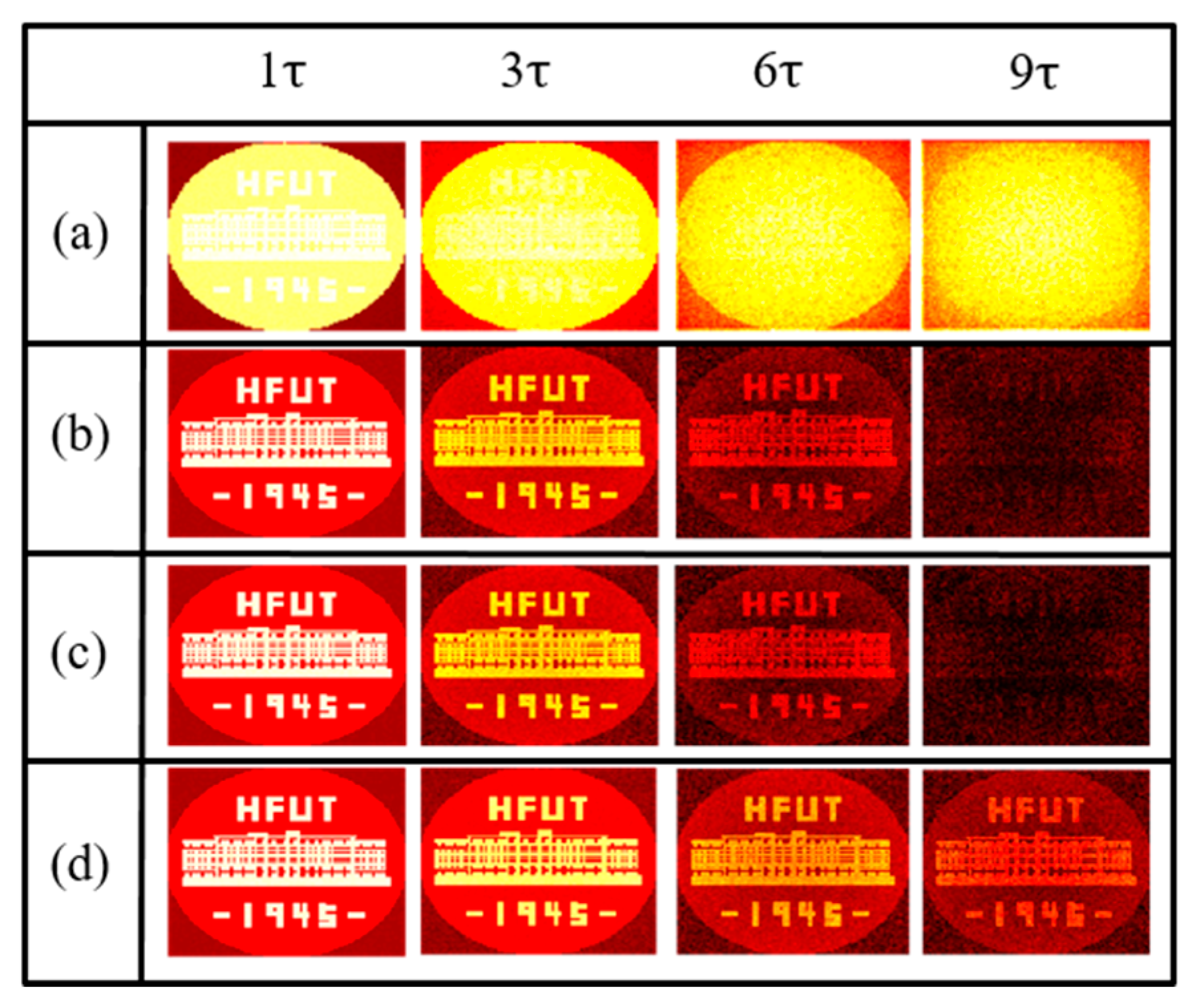
| Figure 5 | |||||
|---|---|---|---|---|---|
| PSNR(dB) | (a) | 12.0078 | 11.6162 | 11.4507 | 10.4056 |
| (b) | 48.0959 | 28.8340 | 18.8228 | 10.5011 | |
| (c) | 48.1036 | 29.7893 | 21.6208 | 11.6163 | |
| (d) | 71.4946 | 36.9868 | 26.2641 | 18.7648 | |
| SSI | (a) | 0.7447 | 0.6948 | 0.6215 | 0.5819 |
| (b) | 0.9956 | 0.9102 | 0.6234 | 0.4662 | |
| (c) | 0.9966 | 0.9179 | 0.6930 | 0.5031 | |
| (d) | 0.9989 | 0.9763 | 0.8602 | 0.7311 | |
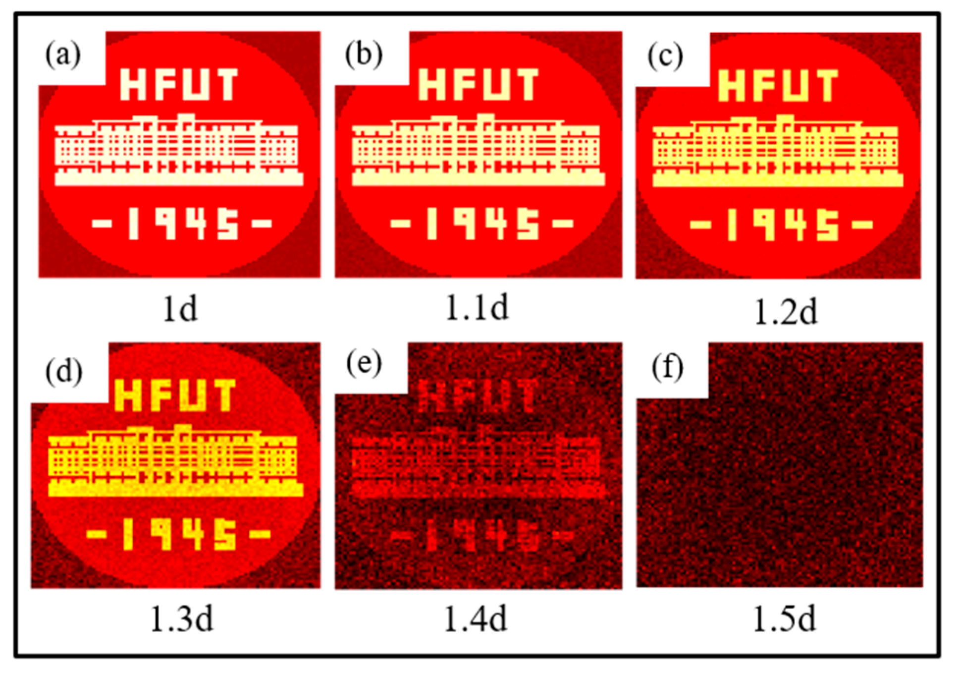
| Figure 7 | 1d | 1.1d | 1.2d | 1.3d | 1.4d | 1.5d |
|---|---|---|---|---|---|---|
| PSNR (dB) | 71.4946 | 34.3927 | 27.4167 | 18.9408 | 10.1266 | 8.0694 |
| SSI | 0.9989 | 0.9918 | 0.9739 | 0.8971 | 0.5491 | 0.3833 |
© 2020 by the authors. Licensee MDPI, Basel, Switzerland. This article is an open access article distributed under the terms and conditions of the Creative Commons Attribution (CC BY) license (http://creativecommons.org/licenses/by/4.0/).
Share and Cite
Wang, X.; Hu, T.; Li, D.; Guo, K.; Gao, J.; Guo, Z. Performances of Polarization-Retrieve Imaging in Stratified Dispersion Media. Remote Sens. 2020, 12, 2895. https://doi.org/10.3390/rs12182895
Wang X, Hu T, Li D, Guo K, Gao J, Guo Z. Performances of Polarization-Retrieve Imaging in Stratified Dispersion Media. Remote Sensing. 2020; 12(18):2895. https://doi.org/10.3390/rs12182895
Chicago/Turabian StyleWang, Xinyang, Tianwei Hu, Dekui Li, Kai Guo, Jun Gao, and Zhongyi Guo. 2020. "Performances of Polarization-Retrieve Imaging in Stratified Dispersion Media" Remote Sensing 12, no. 18: 2895. https://doi.org/10.3390/rs12182895