Abstract
Forest cover mapping based on multi-temporal satellite observations usually uses dozens of features as inputs, which requires huge training data and leads to many ill effects. In this paper, a simple but efficient approach was proposed to map forest cover from time series of satellite observations without using classifiers and training data. This method focuses on the key step of forest mapping, i.e., separation of forests from herbaceous vegetation, considering that the non-vegetated area can be easily identified by the annual maximum vegetation index. We found that the greenness of forests is generally stable during the maturity period, but a similar greenness plateau does not exist for herbaceous vegetation. It means that the mean greenness during the vegetation maturity period of forests should be larger than that of herbaceous vegetation, while its standard deviation should be smaller. A combination of these two features could identify forests with several thresholds. The proposed approach was demonstrated for mapping the extents of different forest types with MODIS observations. The results show that the overall accuracy ranges 91.92–95.34% and the Kappa coefficient is 0.84–0.91 when compared with the reference datasets generated from fine-resolution imagery of Google Earth. The proposed approach can greatly simplify the procedures of forest cover mapping.
1. Introduction
As a critical component of terrestrial ecosystems, forest plays an important role in the global carbon cycle, hydrologic cycle, biodiversity protection and resources supply (e.g., timber and foods) [1,2]. Highly reliable forest distribution is critical for forest conservation, carbon budget estimation and ecosystem service assessment [3,4].
Many global and regional forest cover maps have been generated from satellite data, such as Hansen high-resolution forest cover maps from Landsat images [5], AVHRR/MODIS tree cover maps [6,7], PALSAR forest/non-forest maps [8] and FROM_GLC land cover products [9]. Time series of satellite data have been widely used for forest cover mapping, since they can capture seasonal characteristics of different landcover types and thus improve the separability among them [5,6,7,10,11,12]. However, using time series data greatly increases the number of input features, reaching dozens or even hundreds. The classifiers, such as random forest, decision tree and support vector machine [13,14,15,16], are generally required to extract the forest extent from such a large number of features. They usually need a huge amount of training samples to calibrate the classifiers. With the increase in input features, the required training samples will grow exponentially in order to obtain statistically reliable results, and too many unprocessed features may decrease the generalization ability of the classifier, which may result in the so-called curse of dimensionality [17].
To reduce the dimension of inputs, time series of satellite observations were compacted to new features through statistics analysis, such as the mean, median, maximum, minimum and amplitude of the vegetation index or reflectance during a certain period [18,19,20,21,22,23]. For example, multi-temporal data of AVHRR, MODIS and Landsat ETM+ were transferred to 38, 68 and 113 metrics, respectively, to map global percent tree cover based on regression tree or decision tree algorithms [5,6,7]. These time series metrics include reflectance and NDVI values representing minimum, median, maximum and selected percentile values, mean and amplitude of reflectance and NDVI values for observations between selected percentiles, etc. Complex mathematical transformation was also applied to time series observations to generate new features. The multi-temporal observations of Landsat were converted to 36 spectral-temporal features to discriminate forest types in New England based on a random forest classifier, including 30 harmonic features characterizing mean annual reflectance and seasonal variability, and six phenology metrics quantifying the timing of seasonal events [24]. However, there are still dozens of input features in spite of these simplifications, which require a large number of training samples and may decrease the generalization ability of the classifier. If time series of observations were transformed into features of high discrimination between forests and other vegetation types, it would be possible to extract forest extents with a few features, thereby simplifying the classification procedure.
The aim of this study is to develop a simple approach for forest cover mapping based on time series of optical remote sensing observations. Since non-vegetated areas can be easily excluded using the annual maximum normalized difference vegetation index (NDVI) [25], this paper focuses on the discrimination of forests and herbaceous vegetation. Based on the difference between the spectral seasonal curves of forests and herbaceous vegetation, we proposed two features for discrimination of these two types, namely the mean and standard deviation (SD) of NDVI during the vegetation maturity period. These two features present great separability between forests and herbaceous vegetation, which enable us to map the forest cover effectively by several thresholds without classifiers and training data. The method was demonstrated with four tiles of MODIS observations.
2. Materials and Methods
2.1. Study Area
The proposed method was demonstrated in four MODIS tiles that cover various forest types in different climate zones and latitudes as examples, including h27v05, h25v07, h11v10 and h11v04 (Figure 1). Each tile covers approximately 10 degrees square (at the equator) in sinusoidal projection. (1) H27v05 is located in northern and central China, as well as the northern part of the Korean Peninsula. It covers temperate deciduous broadleaf forests in the Korean Peninsula and mountainous areas of northern and central China, as well as the vast croplands in the North China Plain. (2) H25v07 covers the central and southern parts of India. Monsoon rainforests and evergreen broadleaf forests are distributed in the western coastal, northeastern and eastern mountainous areas of the tile, while the other areas are dominated by croplands or a mosaic of croplands and natural vegetation. (3) H11v10 covers the southwestern part of the Amazon. Tropical rainforests are widely distributed in the upper, middle and lower right parts of the tile. Grasslands and savannas are scattered around forests areas, while barren land is distributed along the coast in the lower left part of the tile. (4) H11v04 covers boreal forests near the Great Lakes in North America. Other areas are mostly croplands, except for a small amount of grasslands in the upper left corner of the tile. The climate is mainly characterized as a temperate monsoon climate, tropical monsoon climate, tropical rainforest/savanna/desert climates and temperate continental climate for tiles h27v05, h25v07, h11v10 and h11v04, respectively.
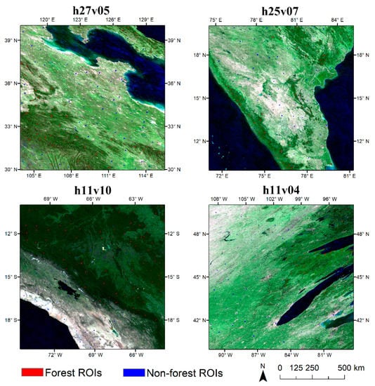
Figure 1.
Study area of four MODIS tiles (h27v05, h25v07, h11v10 and h11v04) and spatial distribution of reference regions of interest (ROIs) used for accuracy assessment. The true-color images show the greenest status of land surface throughout the year in 2010 of four tiles, which were obtained through the minimum red-band composition. For the RGB images, dark green represents forests, light green shows other vegetated area and gray is non-vegetated area.
2.2. Data
2.2.1. MODIS Land Surface Reflectance Data and Preprocessing
The MODIS onboard Terra and Aqua satellites have observed the Earth’s surface every 1 to 2 days since February 2000, which provides the spectral seasonal curves of the land surface and helps to separate forests and herbaceous vegetation. The proposed method was applied to MODIS land surface reflectance product MOD09A1 (Version 6). This product contains global 8-day composite 500 m resolution atmospheric corrected land surface reflectance in bands 1–7. The product is provided on the sinusoidal grid. The land surface reflectance was screened for cloud contamination based on a refined cloud mask method [26]. The snow and water pixels were labeled with the state flags in MOD09A1 products and MODIS land cover type products (MCD12Q1), respectively.
2.2.2. Reference Regions of Interest
The regions of interest (ROIs) were generated from visual interpretation using high-spatial resolution imagery of Google Earth as reference data for results validation (Figure 1). The ROIs were collected for two classes, including forests and non-forests. For forests, we randomly digitalized the patches with tree crown cover of more than 50% and area of exceeding 0.5 ha as forest ROIs, following the criteria used in the definition of forest in this paper (Section 2.3). Non-forest ROIs include that of croplands, grasslands, shrublands, built-up and barren lands. The areas dominated by the above-mentioned types were randomly selected as non-forest ROIs. Since water pixels were labeled with MODIS land cover type products, they were not considered in ROIs generation and results validation. A total of 691 polygon ROIs (84,484 pixels) were generated, including 68, 86, 108 and 105 forest ROIs (40,609 pixels), as well as 63, 71, 98 and 92 non-forest ROIs (43,875 pixels) for tiles h27v05, h25v07, h11v10 and h11v04, respectively. These ROIs were randomly created and distributed across the forest and non-forest areas in each tile.
2.3. Methods
A new method was proposed to distinguish forests and herbaceous vegetation based on the different shape of the NDVI seasonal curve for these two vegetation types. In this paper, forest refers to lands dominated by trees with a canopy cover of greater than 50% and an area of more than 0.5 ha, while herbaceous vegetation refers to areas dominated by herbs, such as grasslands and croplands.
Trees and herbaceous plants show specific seasonal growth trajectories. For evergreen trees, leaves maintain high greenness throughout the year. For deciduous trees, leaves usually grow and senesce quickly in a short period at the beginning and end of the growing season, and the greenness of leaves remains relatively stable during the maturity period. In contrast, for herbaceous plants, leaves generally continue to grow and then senesce slowly during the growing season. Accordingly, the NDVI seasonal curve shows a distinctly different shape for tree-dominated forests and herbaceous vegetation. It is relatively flat during the vegetation maturity period for the former, with NDVI values remaining around high values, while it presents a parabolic shape with an opening downward for the latter. Based on these distinctive seasonal characteristics, two features were proposed to differentiate the two vegetation types, namely the mean and SD of the NDVI during the vegetation maturity period. These two features were generated from annual MODIS observations to map forest cover with the following steps (Figure 2):
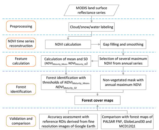
Figure 2.
Workflow of the proposed method for forest cover mapping.
(1) Step 1: reconstruction of NDVI time series. The NDVI was calculated with clear-sky reflectance in red and near-infrared bands from MOD09A1 products, and gaps in its time series were filled and smoothed with the locally adjusted cubic spline capping (LACC) approach [27].
(2) Step 2: calculation of mean and SD of the NDVI during the vegetation maturity period. For each pixel, several maximum NDVIs were selected from annual 8-day MODIS observations. The number of selected maximum NDVIs was determined according to the climate zone of the Koppen–Geiger climate classification. For the tropical climate zone, sixteen maximum NDVIs were selected; for temperate and dry climate zones, the number is twelve; while for continental, polar and alpine climate zones, this number is eight. For each pixel, the mean and SD values were calculated from the selected maximum NDVI values, and are referred to as and , respectively. Experiments show that the number of selected maximum NDVIs does not obviously affect the values of and within a reasonable range.
(3) Step 3: identification of forest and herbaceous vegetation. The non-vegetated regions were firstly masked with an annual maximum NDVI of less than 0.2. Then, the forests and herbaceous vegetation were separated from and based on the threshold method. Most forest pixels are concentrated in regions with high (greater than 0.80) and low values (lower than 0.04). For sparse forest areas, these two features will be slightly lower. In contrast, herbaceous vegetation shows a smaller value of and a larger value of compared to those of forests, the former is mostly less than 0.80 and the latter is up to 0.15. Here, forest was identified with the following rules:
2.4. Validation and Comparison to Existing Datasets
The results of our algorithm were evaluated with the ROIs derived from high-resolution images of Google Earth (Figure 1, Section 2.2.2). A confusion matrix was calculated based on the ROIs and extracted forest cover maps. The overall, user’s and producer’s accuracies as well as the Kappa coefficients were estimated to evaluate the accuracy of the extracted forest cover maps.
The derived forest cover maps were also compared with the PALSAR forest/non-forest map (FNF, 25 m) [8], 30 m Global Land Cover Data Sets (GlobeLand30, 30 m) [28] and MODIS land cover products (MCD12Q1, 500 m) [19]. The two high-resolution datasets were aggregated to 500 m resolution by calculating the percentage of forest pixels in each 500 m grid, and those grids with a forest percentage of more than 60% were labeled as forests for comparison. The MCD12Q1 Version 6 product from the International Geosphere-Biosphere Programme (IGBP) classification scheme (Type 1) was grouped into four classes, including forests, non-forests, non-vegetated areas and water. The percentage of our results and MCD12Q1 relative to the areas labeled as forest both in the two high-resolution datasets were calculated to evaluate the consistency of datasets.
3. Results
3.1. Different Shape of NDVI Seasonal Curve between Forests and Herbacous Vegetation
Figure 3 illustrates the different shapes of the NDVI seasonal curves between forests and herbaceous vegetation. The smoothed MODIS NDVI temporal profiles during the period 2010–2017 were presented for five BELMANIP sites and one monsoon rainforest site in India, including deciduous broadleaf forest (DBF) at Morgan Monroe State Forest in USA, evergreen broadleaf forest (EBF) at AekLoba in Sumatra, deciduous needleleaf forest (DNF) at Krasnoyarsk in Russia, evergreen needleleaf forest (ENF) at Howland in USA, tropical semi-deciduous rainforest (TSDRF) at Budongo Forest in Uganda and monsoon rainforest (MRF) at a site in India (Table 1). For each forest site, a cropland site was selected nearby based on Google Earth high-resolution images, and its smoothed NDVI series were also displayed in Figure 3 to represent the seasonal curve of herbaceous vegetation.
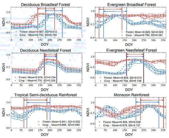
Figure 3.
NDVI time series for various forest and adjacent cropland sites from 2010 to 2017, including deciduous broadleaf forest (Morgan Monroe State Forest, USA), evergreen broadleaf forest (AekLoba, Sumatra), deciduous needleleaf forest (Krasnoyarsk, Russia), evergreen needleleaf forest (Howland, USA), tropical semi-deciduous rainforest (Budongo Forest, Uganda) and monsoon rainforest (78.79° N, 15.56° E, India). Detailed information is shown in Table 1. Red and blue represent forests and crops, respectively, and the periods indicated by the arrows are the vegetation maturity period. The values of mean and SD in the figure refer to and , respectively.

Table 1.
Information of forest and adjacent cropland sites in Figure 3. Fine-resolution images from Google Earth are also shown for each forest and cropland site.
We found that the NDVI seasonal curves show distinctly different shapes for forests and herbaceous vegetation during the vegetation maturity period. A significant greenness plateau is observed during the vegetation maturity period for most forest sites except DNF, with NDVI values being stable around 0.8 or even above. In contrast, the cropland NDVI series show a parabolic shape with an opening downward during the maturity period, with notable variations in NDVI values, which significantly differ from those of forests. The of forests is generally higher than that of crops, while its is much smaller. For forests, the of all six sites is above 0.8, while is mostly around 0.02, with the maximum value not exceeding 0.04. For neighboring crops, is around 0.7, with the maximum value being no more than 0.76, while most SD values are above 0.05, and it is even greater than 0.10 for DBF, ENF and MRF. For DNF, although its NDVI curve is similar to that of neighboring cropland, differences are still observed for the two features compared to that of cropland.
3.2. Contrast of Mean and SD of NDVI during the Vegetation Maturity Period between Forests and Herbaceous Vegetaiton
Figure 4 displays maps of and in 2010 for the four MODIS tiles, including h27v05, h25v07, h11v10 and h11v04. The results demonstrate that these two features present notable differences between forest and non-forest at regional scale, according to the true color imagery in Figure 1. For the forest areas (dark green in RGB images in Figure 1), the value of is generally above 0.8, and is below 0.02. For tropical rainforest (h11v10) with a dense canopy, the is above 0.85 or even 0.9, while is around 0.01. In contrast, for crops and grasses (light green in RGB images in Figure 1), the is generally below 0.8, and the SD value is above 0.035. For sparsely vegetated areas (gray in RGB images in Figure 1), such as the central part of h25v07, upper left corner of h11v04 and lower left zone along the forest areas of h11v10, the is usually below 0.6, which is much lower than that of dense vegetation. Significant differences of the two features between forest and other landcover types could contribute to forest classification. For tropical regions, including h25v07 and h11v10, the of herbaceous vegetation is generally lower than that in middle and high latitudes, but its value is still significantly lower than that of forests. Combining the two features can effectively distinguish forest and herbaceous vegetation in these regions.
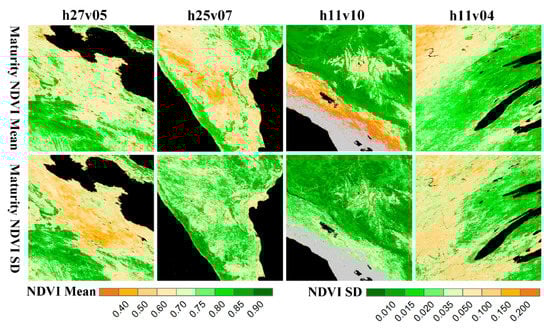
Figure 4.
Maps of and for four MODIS tiles in 2010, including h27v05, h25v07, h11v10 and h11v04. The gray color refers to non-vegetated areas.
3.3. Extracted Forest Cover Maps and Accuracy Assessment
Figure 5 illustrates the extracted forest cover maps in 2010 for the four tiles. The total area of forests estimated is 2.443, 1.624, 5.187 and 2.311 million ha for h27v05, h25v07, h11v10 and h11v04, respectively. The forest maps are in good agreement with the distribution shown in the true color map (Figure 1). Our algorithm successfully identified the forest areas in four tiles, including the temperate forests in mountainous regions in the lower left part of h27v05 and in the Korean Peninsula in the upper right corner, tropical monsoon forests and evergreen broadleaf forests in the west coast and northeast parts of India in h25v07, tropical rainforests that are widely distributed in h11v10 and the sparse boreal forests around the Great Lakes in h11v04.
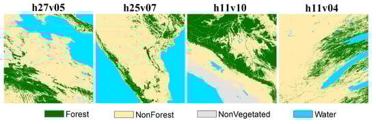
Figure 5.
Forest cover maps derived with the proposed method in 2010 for h27v05, h25v07, h11v10 and h11v04.
The extracted forest cover maps were validated with the reference ROIs generated from the Google Earth high-resolution images (Section 2.2.2). The confusion matrix demonstrates that the proposed method has a reasonably high accuracy for mapping forests in the study area, with the overall accuracy exceeding 91% for the four tiles (Table 2). The overall accuracies are 95.34%, 94.02%, 93.83% and 91.92% for h27v05, h25v07, h11v10 and h11v04, respectively, while the Kappa coefficients are 0.9062, 0.8803, 0.8769 and 0.8363, respectively. The user’s accuracies of forests are all above 92% for four tiles, while their producer’s accuracies are slightly lower, which ranges from 88.36% to 92.32%. This indicates the possibility of an underestimation of forest cover compared to the reference ROIs. Higher overall accuracies are found for tiles h27v05, h25v07 and h11v10 than h11v04, suggesting that the proposed method may perform better in middle-low latitudes than in high latitudes.
Table 2.
Accuracy assessment of the extracted forest cover maps using reference ROIs from high-resolution images of Google Earth for tiles h27v05, h25v07, h11v10 and h11v04 in 2010.
3.4. Comparison to Existing Datasets
The extracted forest cover maps were compared to those of MCD12Q1, PALSAR FNF and GlobeLand30 products (Figure 6). The results show that the spatial distribution of our results is generally in good agreement with that of the two high-resolution products, suggesting that the proposed method can identify the forests reasonably.
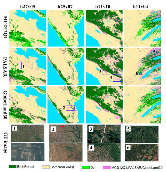
Figure 6.
Comparison of the extracted forest cover maps with MCD12Q1, PALSAR FNF and GlobeLand30 products in 2010 for h27v05, h25v07, h11v10 and h11v04. The gray and blue colors refer to non-vegetated areas and waterbodies. Google Earth (GE) high-resolution images are also shown for six subregions.
For temperate deciduous broadleaf forests in h27v05 and evergreen and monsoon rainforests in h25v07, the spatial distribution and total area of forests of our results (2.443 and 1.624 million ha for h27v05 and h25v07, respectively) are consistent with those of PALSAR FNF (2.457 and 1.718 million ha) and GlobeLand30 (2.589 and 1.803 million ha). Our results identified 87.60% and 81.99% of the areas where both of the two high-resolution products are labeled as forests for the two tiles, respectively. In Regions 1 and 2 in Figure 6, the croplands in the North China Plain and central India were falsely detected as forests in PALSAR FNF and GlobeLand30, respectively, while they were correctly differentiated by our method. For MCD12Q1, the area of forests (1.175 and 0.780 million ha) is about half of the other three datasets, and only 53.89% and 50.01% of areas labeled as forests both in the two high-resolution products were classified as forests (Table 2). The inconsistencies were mainly distributed in the areas with low tree coverage, where the definition of forest greatly affects the extracted forest extent.
For tropical rainforests in h11v10, the spatial distribution of forests is basically consistent among the four datasets, with the total area of forests with our algorithm (5.187 million ha) being slightly smaller than other products (6.026 million ha for MCD12Q1, 6.308 million ha for PALSAR and 6.064 million ha for GlobeLand30). Our results identified 86.87% of the areas where both of the two high-resolution forest datasets were labeled as forests. Most omission occurs in the edges of wide forest areas. Google Earth high-resolution images show that these areas are mainly located in rugged mountainous areas, with moderate or low tree coverage (Regions 3 and 4 in Figure 6).
For boreal forests in h11v04, substantial differences are presented in forest distribution among the four datasets, with the area ranging from 1.729 (MCD12Q1) to 3.464 million ha (PALSAR). The total forest area detected by our algorithm is 2.311 million ha. Our method identified 70.03% of the areas where both of the two high-resolution products were labeled as forests. Some forest pixels were not identified in our results in the upper right corner of the tile, where a large number of lakes mixed in forests (Region 5 in Figure 6). In this region, the forest cover is fragmented and the NDVI seasonal curve is altered by water, resulting in difficulties in forest identification with coarse MODIS data (500 m resolution). In the central part of the tile, where forests and croplands are mixed, our method detected the forests successfully, while other products may miss part of forest pixels in such a complex landscape (Region 6 in Figure 6).
4. Discussion
In this paper, the satellite time series observations were simplified to two features for forest mapping, i.e., mean and SD of the NDVI during the vegetation maturity period. These two features characterize the different shapes of greenness seasonal curves between forests and herbaceous vegetation, which enable us to extract the forest extent even with several thresholds. The proposed method is simple and efficient, making it suitable for rapid forest identification at regional scale. The performance of classification could be improved easily by adjusting the thresholds according to local vegetation status. The two features can also be used as inputs of landcover classification. With a combination of other features and classifiers, it would help to identify forest biomes. The proposed method can be applied for other optical sensors with high temporal resolution, such as AVHRR, VEGETATION and Sentinel-2. For satellites with low temporal resolution, such as Landsat, this method may also be applicable with reconstructed seasonal sequences using multi-sensor fusion, multi-year composition or time series modeling.
Several factors may affect the performance of our algorithm, such as clouds, waterbodies and evergreen shrublands. Clouds and other noise will significantly increase the fluctuations of NDVI seasonal curves, and consequently increase the value of , which may result in the omission of forests. The noise in satellite observations should be excluded with a strict cloud detection algorithm before calculation of the two features. Specifically, in areas with frequent cloud coverage, it is difficult to obtain reliable seasonal curves of the NDVI due to sparse clear-sky observations, which may result in unrealistic detection. In areas where forests and waterbodies are mixed, water decreases the NDVI value and alters its seasonal curve, which may affect the performance of our algorithm. High-temporal and spatial resolution observation would help to improve the classification in these areas. In areas with evergreen shrubs, the SD values of the NDVI may be close to that of forests during the vegetation maturity period, but the mean NDVI values of the former are often lower than that of the latter, which helps to discriminate forests.
There are many definitions of forest in use, which differ in the tree canopy cover, area and tree height, etc. The Food and Agriculture Organization of the United Nations (FAO) defines forest as land spanning more than 0.5 ha with trees higher than 5 m and canopy cover of greater than 10%, with the absence of other predominant land uses [29]. PALSAR and GlobeLand30 use the definition of FAO [8,23], which can identify sparse forests with the threshold of tree canopy cover of 10%. The MCD12Q1 IGBP class defines forest as the area dominated by trees with tree cover of greater than 60% and canopy height above 2 m, and those pixels with tree cover ranging 10–60% are classified to woody savannas and savannas [19]. Here, the forest identified by our algorithm is areas with tree canopy cover of more than 50%. Our method is based on the difference of the seasonal growth characteristics between trees and herbaceous plants. This difference may be too small to be distinguished with satellite observation for those pixels with a low proportion of trees. When the tree crown cover reaches up to 50%, a distinct difference is presented for the MODIS NDVI curves between forests and herbaceous vegetation, which helps to extract the forest extent reliably. Different forest definitions may lead to inconsistencies in satellite forest cover products, especially in areas with low tree coverage, such as sparse forests and forest edges (Section 3.4). The forest area detected by MCD12Q1 and our algorithm is generally lower than that of PALSAR and GlobeLand30, which may be related to the higher thresholds of tree canopy cover used compared with the latter two products.
5. Conclusions
This paper developed a simple but efficient method for forest cover mapping with optical sensor data. Based on the differences in the shape of greenness seasonal curves between the forests and herbaceous vegetation, this method simplifies time series of satellite data into two features, namely the mean and standard derivation of the NDVI during the vegetation maturity period. The forest extent was extracted with several thresholds from these two features, which present great separability between forests and herbaceous vegetation. This method was demonstrated for forest cover mapping with MODIS observations in four tiles, which cover different forest types and latitudes. The results show that it could efficiently identify temperate deciduous broadleaf forests, tropical rainforests and monsoon rainforests in middle-low latitudes without classifiers and training data. Compared with the reference ROIs from high-resolution images of Google Earth, the overall, producer’s and user’s accuracies were up to 91.92–95.34%, 88.36–92.32% and 92.86–99.48%, respectively. The extracted forest cover maps are generally consistent with those of high-resolution forest maps of PALSAR and GlobeLand30. The method successfully identified 87.60%, 81.99% and 86.87% of the areas, where both of the high-resolution PALSAR FNF and GlobeLand30 products were labeled as forests, for the three tiles, respectively. For boreal forests in high latitudes, disparities were found in forest distribution among the four datasets due to the sparse tree coverage and vast small lakes, and 70.03% of forest areas in the two high-resolution products was identified by our algorithm. Frequent clouds, low tree coverage and mixed distributed waterbodies may increase the uncertainty in classification.
Further research can be done to apply this method to other sensors, such as AVHRR, Sentinel-2 and Landsat. The application of AVHRR observations would help to evaluate the historical forest cover changes. Additionally, high-spatial and temporal resolution datasets have been constructed by fusing multi-sensor data or time series modeling [30,31]. Our method can also be used for those reconstructed datasets whose fine spatial resolution would help to improve the forest cover mapping.
Author Contributions
Conceptualization, R.L.; methodology, R.L.; software, R.L. and Y.L.; formal analysis, R.L. and Y.L.; investigation, Y.L.; validation, Y.L.; resources, R.L.; data curation, R.L.; writing—original draft preparation, Y.L.; writing—review and editing, R.L. and Y.L.; visualization, Y.L.; supervision, R.L.; project administration, R.L.; funding acquisition, R.L. All authors have read and agreed to the published version of the manuscript.
Funding
This research was funded in part by the Strategic Priority Research Program of the Chinese Academy of Sciences (XDA19080303); in part by the National Key Research and Development Program of China (2019YFA0606601, 2016YFA0600201); and in part by the Youth Innovation Promotion Association of Chinese Academy of Sciences (2019056).
Acknowledgments
The authors would like to thank the NASA Land Processes Distributed Active Archive Center for providing the MODIS products, and Japan Aerospace Exploration Agency for providing ALOS PALSAR FNF dataset.
Conflicts of Interest
The authors declare no conflict of interest.
References
- Bonan, G.B. Forests and climate change: Forcings, feedbacks, and the climate benefits of forests. Science 2008, 320, 1444–1449. [Google Scholar] [CrossRef] [PubMed]
- Pimm, S.L.; Jenkins, C.N.; Abell, R.; Brooks, T.M.; Gittleman, J.L.; Joppa, L.N.; Raven, P.H.; Roberts, C.M.; Sexton, J.O. The biodiversity of species and their rates of extinction, distribution, and protection. Science 2014, 344, 987–992. [Google Scholar] [CrossRef] [PubMed]
- Qin, Y.W.; Xiao, X.M.; Dong, J.W.; Zhang, Y.; Wu, X.C.; Shimabukuro, Y.; Arai, E.; Biradar, C.; Wang, J.; Zou, Z.H.; et al. Improved estimates of forest cover and loss in the Brazilian Amazon in 2000–2017. Nat. Sustain. 2019, 2, 764–772. [Google Scholar] [CrossRef]
- Tong, X.W.; Brandt, M.; Yue, Y.M.; Ciais, P.; Jepsen, M.R.; Penuelas, J.; Wigneron, J.P.; Xiao, X.M.; Song, X.P.; Horion, S.; et al. Forest management in southern China generates short term extensive carbon sequestration. Nat. Commun. 2020, 11. [Google Scholar] [CrossRef]
- Hansen, M.C.; Potapov, P.V.; Moore, R.; Hancher, M.; Turubanova, S.A.; Tyukavina, A.; Thau, D.; Stehman, S.V.; Goetz, S.J.; Loveland, T.R.; et al. High-Resolution Global Maps of 21st-Century Forest Cover Change. Science 2013, 342, 850–853. [Google Scholar] [CrossRef]
- Hansen, M.C.; DeFries, R.S. Detecting long-term global forest change using continuous fields of tree-cover maps from 8-km advanced very high resolution radiometer (AVHRR) data for the years 1982–99. Ecosystems 2004, 7, 695–716. [Google Scholar] [CrossRef]
- Hansen, M.C.; DeFries, R.S.; Townshend, J.R.G.; Carroll, M.; Dimiceli, C.; Sohlberg, R.A. Global Percent Tree Cover at a Spatial Resolution of 500 Meters: First Results of the MODIS Vegetation Continuous Fields Algorithm. Earth Interact. 2003, 7, 1–15. [Google Scholar] [CrossRef]
- Shimada, M.; Itoh, T.; Motooka, T.; Watanabe, M.; Shiraishi, T.; Thapa, R.; Lucas, R. New global forest/non-forest maps from ALOS PALSAR data (2007–2010). Remote Sens. Environ. 2014, 155, 13–31. [Google Scholar] [CrossRef]
- Gong, P.; Wang, J.; Yu, L.; Zhao, Y.C.; Zhao, Y.Y.; Liang, L.; Niu, Z.G.; Huang, X.M.; Fu, H.H.; Liu, S.; et al. Finer resolution observation and monitoring of global land cover: First mapping results with Landsat TM and ETM+ data. Int. J. Remote Sens. 2013, 34, 2607–2654. [Google Scholar] [CrossRef]
- Gomez, C.; White, J.C.; Wulder, M.A. Optical remotely sensed time series data for land cover classification: A review. ISPRS J. Photogramm. Remote Sens. 2016, 116, 55–72. [Google Scholar] [CrossRef]
- Zhang, Y.H.; Ling, F.; Foody, G.M.; Ge, Y.; Boyd, D.S.; Li, X.D.; Du, Y.; Atkinson, P.M. Mapping annual forest cover by fusing PALSAR/PALSAR-2 and MODIS NDVI during 2007–2016. Remote Sens. Environ. 2019, 224, 74–91. [Google Scholar] [CrossRef]
- Emmanuelle, C.; Jean-Philippe, D.; Mar, B.; Laurence, H.; Véronique, C. Improved forest-cover mapping based on MODIS time series and landscape stratification. Int. J. Remote Sens. 2017, 38, 1865–1888. [Google Scholar] [CrossRef]
- Matasci, G.; Hermosilla, T.; Wulder, M.A.; White, J.C.; Coops, N.C.; Hobart, G.W.; Zald, H.S.J. Large-area mapping of Canadian boreal forest cover, height, biomass and other structural attributes using Landsat composites and lidar plots. Remote Sens. Environ. 2018, 209, 90–106. [Google Scholar] [CrossRef]
- Xu, Y.D.; Yu, L.; Li, W.; Ciais, P.; Cheng, Y.Q.; Gong, P. Annual oil palm plantation maps in Malaysia and Indonesia from 2001 to 2016. Earth Syst. Sci. Data 2020, 12, 847–867. [Google Scholar] [CrossRef]
- Nwobi, C.; Williams, M.; Mitchard, E.T.A. Rapid Mangrove Forest Loss and Nipa Palm (Nypa fruticans) Expansion in the Niger Delta, 2007–2017. Remote Sens. 2020, 12, 2344. [Google Scholar] [CrossRef]
- Potapov, P.; Turubanova, S.; Hansen, M.C. Regional-scale boreal forest cover and change mapping using Landsat data composites for European Russia. Remote Sens. Environ. 2011, 115, 548–561. [Google Scholar] [CrossRef]
- Trunk, G.V. A Problem of Dimensionality: A Simple Example. IEEE Trans. Pattern Anal. Mach. Intell. 1979, 1, 306–307. [Google Scholar] [CrossRef]
- Hansen, M.C.; Defries, R.S.; Townshend, J.R.G.; Sohlberg, R. Global land cover classification at 1km spatial resolution using a classification tree approach. Int. J. Remote Sens. 2000, 21, 1331–1364. [Google Scholar] [CrossRef]
- Friedl, M.A.; Sulla-Menashe, D.; Tan, B.; Schneider, A.; Ramankutty, N.; Sibley, A.; Huang, X.M. MODIS Collection 5 global land cover: Algorithm refinements and characterization of new datasets. Remote Sens. Environ. 2010, 114, 168–182. [Google Scholar] [CrossRef]
- DeFries, R.; Hansen, M.; Townshend, J. Global discrimination of land cover types from metrics derived from AVHRR pathfinder data. Remote Sens. Environ. 1995, 54, 209–222. [Google Scholar] [CrossRef]
- Lloyd, D. A phenological classification of terrestrial vegetation cover using shortwave vegetation index imagery. Int. J. Remote Sens. 1990, 11, 2269–2279. [Google Scholar] [CrossRef]
- Reed, B.C.; Brown, J.F.; Vanderzee, D.; Loveland, T.R.; Merchant, J.W.; Ohlen, D.O. Measuring phenological variability from satellite imagery. J. Veg. Sci. 1994, 5, 703–714. [Google Scholar] [CrossRef]
- Gong, P.; Liu, H.; Zhang, M.N.; Li, C.C.; Wang, J.; Huang, H.B.; Clinton, N.; Ji, L.Y.; Li, W.Y.; Bai, Y.Q.; et al. Stable classification with limited sample: Transferring a 30-m resolution sample set collected in 2015 to mapping 10-m resolution global land cover in 2017. Sci. Bull. 2019, 64, 370–373. [Google Scholar] [CrossRef]
- Pasquarella, V.J.; Holden, C.E.; Woodcock, C.E. Improved mapping of forest type using spectral-temporal Landsat features. Remote Sens. Environ. 2018, 210, 193–207. [Google Scholar] [CrossRef]
- Qin, Y.W.; Xiao, X.M.; Dong, J.W.; Zhang, G.L.; Shimada, M.; Liu, J.Y.; Li, C.G.; Kou, W.L.; Moore, B. Forest cover maps of China in 2010 from multiple approaches and data sources: PALSAR, Landsat, MODIS, FRA, and NFI. ISPRS J. Photogramm. Remote Sens. 2015, 109, 1–16. [Google Scholar] [CrossRef]
- Liu, R.G.; Liu, Y. Generation of new cloud masks from MODIS land surface reflectance products. Remote Sens. Environ. 2013, 133, 21–37. [Google Scholar] [CrossRef]
- Chen, J.M.; Deng, F.; Chen, M.Z. Locally adjusted cubic-spline capping for reconstructing seasonal trajectories of a satellite-derived surface parameter. IEEE Trans. Geosci. Remote Sens. 2006, 44, 2230–2238. [Google Scholar] [CrossRef]
- Chen, J.; Chen, J.; Liao, A.P.; Cao, X.; Chen, L.J.; Chen, X.H.; He, C.Y.; Han, G.; Peng, S.; Lu, M.; et al. Global land cover mapping at 30 m resolution: A POK-based operational approach. ISPRS J. Photogramm. Remote Sens. 2015, 103, 7–27. [Google Scholar] [CrossRef]
- Food and Agriculture Organization. Global Forest Resources Assessment 2020. Rome, 2020. Available online: https://doi.org/10.4060/ca8753en (accessed on 26 August 2020).
- Gao, F.; Masek, J.; Schwaller, M.; Hall, F. On the blending of the Landsat and MODIS surface reflectance: Predicting daily Landsat surface reflectance. IEEE Trans. Geosci. Remote Sens. 2006, 44, 2207–2218. [Google Scholar] [CrossRef]
- Yan, L.; Roy, D.P. Spatially and temporally complete Landsat reflectance time series modelling: The fill-and-fit approach. Remote Sens. Environ. 2020, 241. [Google Scholar] [CrossRef]


© 2020 by the authors. Licensee MDPI, Basel, Switzerland. This article is an open access article distributed under the terms and conditions of the Creative Commons Attribution (CC BY) license (http://creativecommons.org/licenses/by/4.0/).