Machine Learning and the End of Atmospheric Corrections: A Comparison between High-Resolution Sea Surface Salinity in Coastal Areas from Top and Bottom of Atmosphere Sentinel-2 Imagery


Abstract
1. Introduction
- if →,
- if → and
- if →.
2. Methodology
2.1. Sentinel-2 Level-1C and Level-2A Imagery
2.2. Copernicus Marine Environmental Monitoring Service In Situ Data
2.3. Satellite–In Situ Matching Process and Neural Network Approach
- In situ data containing salinity since May 2017 to 2020 (i.e., 3 years of data, linked to the Sentinel-2 L2A availability) is downloaded from the Copernicus Marine In Situ data portal [24]. Data are extracted from the Global component, but also from the different seas: Arctic, Baltic, Black Sea, Iberian–Biscay–Ireland, Mediterranean and Northwest Shelf seas.
- For each in situ point coordinate, Sentinel-2 L1C and L2A image collections are filtered to the tiles that contain the point on the day and time when the measurement was taken. The image is only considered if the in situ measurement was taken within 1 hour of the Sentinel-2 pass time.
- If there are any valid tiles for that point, these are clipped in sections of area m m, centred in the point location to obtain high-resolution estimators of SSS.
- The time difference between the in situ measurement and the satellite image is recorded. In case of multiple tiles covering the point of interest, the matched data is sorted by time difference, and the match with the smallest time difference is selected.
- A table containing satellite data (band information and metadata) and equivalent SSS in situ information for each valid point is composed for both L1C and L2A collections.
- Band QA60 containing a cloud mask has been used as a filter to select points only with a clear sky (i.e., points were clouds are persistent have not been considered: no opaque clouds or cirrus clouds are present).
- Duplicates are dropped.
- Matching datasets for L1C and L2A are compared and filtered to ensure the same information is available for both.
- Outlier removal: any values outside a range of standard deviations are not considered. Assuming data follows a normal distribution, any data points in the tail of the distribution over 3 standard deviations from the mean represent ~ of the information.
- Data normalisation is conducted using , where is the normalised value, X is the original value, is the minimum value of the normalised vector and is the maximum value of the normalised vector. Normalised data is fed to the neural network.
- Coefficient of determination ():
- Mean Absolute Error (MAE):
- Most common error (), defined as the expectation (or mean) of the error distribution:
3. Results
- Scenario 1: Baseline scenario.
- Scenario 2: Temperature included as input.
- Scenario 3: Latitude included as input.
- Scenario 4: Longitude included as input.
3.1. Interpolation
3.1.1. Experiment 1
3.1.2. Experiment 2
3.1.3. Experiment 3
3.1.4. Experiment 4
3.2. Extrapolation
4. Discussion: Evaluation and Comparison of Outputs from L1C and L2A in Complete Tiles
4.1. Kuwait Bay, Persian Gulf
4.2. Mouth of the Amazon River, West Atlantic
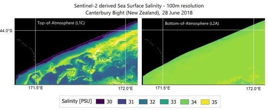
4.3. Canterbury Bight, South Pacific
5. Conclusions
Funding
Conflicts of Interest
References
- European Space Agency. Sentinel—2 Data Products. 2020. Available online: https://sentinel.esa.int/web/sentinel/missions/sentinel-2/data-products (accessed on 10 June 2020).
- ESA. Sentinel—2 User Handbook; ESA Standard Documents; ESA: Paris, France, 2015; Available online: https://sentinel.esa.int/documents/247904/685211/Sentinel-2_User_Handbook (accessed on 10 June 2020).
- Liang, S.; Li, X.; Wang, J. (Eds.) Chapter 5—Atmospheric Correction of Optical Imagery. In Advanced Remote Sensing; Academic Press: Boston, FL, USA, 2012; pp. 111–126. Available online: http://www.sciencedirect.com/science/article/pii/B9780123859549000058 (accessed on 10 June 2020).
- MODTRAN 5.2.0.0 User’s Manual. In Advanced Remote Sensing; Spectral Sciences, Inc.: Burlington, MA, USA, 2008.
- Applications, R. ATCOR—Code Comparison. 2020. Available online: https://www.rese.ch/software/atcor/compare.html (accessed on 10 June 2020).
- European Space Agency. Sentinel—2 Level—2A Processing Overview. 2020. Available online: https://earth.esa.int/web/sentinel/technical-guides/sentinel-2-msi/level-2a-processing (accessed on 10 June 2020).
- European Space Agency. Sen2Cor. 2020. Available online: http://step.esa.int/main/third-party-plugins-2/sen2cor/ (accessed on 10 June 2020).
- Pflug, B.; Main-Knorn, M.; Bieniarz, J.; Debaecker, V.; Louis, J. Early Validation of Sentinel-2 L2A Processor and Products. In Proceedings of the Living Planet Symposium, Prague, Czech Republic, 9–13 May 2016. [Google Scholar]
- Satellite Imaging Corporation. ATCOR. 2020. Available online: https://www.satimagingcorp.com/services/atcor/ (accessed on 10 June 2020).
- Kremezi, M.; Karathanassi, V. Correcting the BRDF Effects on Sentinel-2 Ocean Images. In Proceedings of the Seventh International Conference on Remote Sensing and Geoinformation of the Environment (RSCy2019), 111741C, Paphos, Cyprus, 18–21 March 2019. [Google Scholar] [CrossRef]
- European Space Agency. Level 2A Input Output Data Definition. 2020. Available online: https://step.esa.int/thirdparties/sen2cor/2.5.5/docs/S2-PDGS-MPC-L2A-IODD-V2.5.5.pdf (accessed on 10 June 2020).
- Sterckx, S.; Knaeps, E.; Ruddick, K. Detection and correction of adjacency effects in hyperspectral airborne data of coastal and inland waters: The use of the near infrared similarity spectrum. Int. J. Remote Sens. 2011, 32, 6479–6505. [Google Scholar] [CrossRef]
- Richter, R.; Louis, J.; Berthelot, B. Sentinel-2 MSI—Level 2A Products Algorithm Theoretical Basis Document. 2011. Available online: https://earth.esa.int/c/document_library/get_file?folderId=349490&name=DLFE-4518.pdf (accessed on 10 June 2020).
- Barre, H.M.J.P.; Duesmann, B.; Kerr, Y.H. SMOS: The Mission and the System. IEEE Trans. Geosci. Remote Sens. 2008, 46, 587–593. [Google Scholar] [CrossRef]
- Le Vine, D.M.; Lagerloef, G.S.E.; Ral Colomb, F.; Yueh, S.H.; Pellerano, F.A. Aquarius: An Instrument to Monitor Sea Surface Salinity From Space. IEEE Trans. Geosci. Remote Sens. 2007, 45, 587–593. [Google Scholar] [CrossRef]
- Siddorn, J.; Bowers, D.; Hoguane, A. Detecting the Zambezi River Plume using Observed Optical Properties. Mar. Pollut. Bull. 2001, 42, 942–950. [Google Scholar] [CrossRef]
- Aarup, T.; Holt, N.; Højerslev, N. Optical measurements in the North Sea-Baltic Sea transition zone. II. Water mass classification along the Jutland west coast from salinity and spectral irradiance measurements. Cont. Shelf Res. 1996, 16, 1343–1353. [Google Scholar] [CrossRef]
- Warnock, R.E.; Gieskes, W.W.; van Laar, S. Regional and seasonal differences in light absorption by yellow substance in the Southern Bight of the North Sea. J. Sea Res. 1999, 42, 169–178. [Google Scholar] [CrossRef]
- McKee, D.; Cunningham, A.; Jones, K. Simultaneous Measurements of Fluorescence and Beam Attenuation: Instrument Characterization and Interpretation of Signals from Stratified Coastal Waters. Estuar. Coast. Shelf Sci. 1999, 48, 51–58. [Google Scholar] [CrossRef]
- Bowers, D.; Harker, G.; Smith, P.; Tett, P. Optical Properties of a Region of Freshwater Influence (The Clyde Sea). Estuar. Coast. Shelf Sci. 2000, 50, 717–726. [Google Scholar] [CrossRef]
- Sullivan, S.A. Experimental Study of the Absorption in Distilled Water, Artificial Sea Water, and Heavy Water in the Visible Region of the Spectrum. J. Opt. Soc. Am. 1963, 53, 962–968. [Google Scholar] [CrossRef]
- Medina-Lopez, E.; Urena-Fuentes, L. High-Resolution Sea Surface Temperature and Salinity in Coastal Areas Worldwide from Raw Satellite Data. Remote Sens. 2019, 11, 2191. [Google Scholar] [CrossRef]
- Chen, S.; Hu, C. Estimating sea surface salinity in the northern Gulf of Mexico from satellite ocean colour measurements. Remote Sens. Environ. 2017, 201, 115–132. [Google Scholar] [CrossRef]
- Copernicus. Copernicus, Europe’s Eyes of Earth. 2020. Available online: https://www.copernicus.eu/en (accessed on 10 June 2020).
- Copernicus Marine Environment Monitoring Service. 2020. Available online: https://marine.copernicus.eu/ (accessed on 10 June 2020).
- Google. Google Earth Engine. 2020. Available online: https://code.earthengine.google.com (accessed on 10 June 2020).
- Gorelick, N.; Hancher, M.; Dixon, M.; Ilyushchenko, S.; Thau, D.; Moore, R. Google Earth Engine: Planetary-scale geospatial analysis for everyone. Remote Sens. Environ. 2017, 202, 18–27. [Google Scholar] [CrossRef]
- Srivastava, R.; Greff, K.; Schmidhuber, J. Highway networks. arXiv 2015, arXiv:1505.00387. [Google Scholar]
- Toomer, G.J. The Solar Theory of az-Zarqal A History of Errors. Centaurus 1969, 14, 306–336. [Google Scholar] [CrossRef]


| Level-1C | Level-2A | Resolution (m) | Wavelength (nm) | Description |
|---|---|---|---|---|
| B1 | B1 | 60 | 443.9 | Aerosols |
| B2 | B2 | 10 | 496.6 | Blue |
| B3 | B3 | 10 | 560 | Green |
| B4 | B4 | 10 | 664.5 | Red |
| B5 | B5 | 20 | 703.9 | Red Edge 1 |
| B6 | B6 | 20 | 740.2 | Red Edge 2 |
| B7 | B7 | 20 | 782.5 | Red Edge 3 |
| B8 | B8 | 10 | 835.1 | NIR |
| B8a | B8a | 20 | 864.8 | Red Edge 4 |
| B9 | B9 | 60 | 945 | Water vapour |
| B10 (*) | - | 60 | 1373.5 | Cirrus |
| B11 | B11 | 20 | 1613.7 | SWIR1 |
| B12 | B12 | 20 | 2202.4 | SWIR2 |
| QA60 (*) | QA60 | 60 | - | Cloud mask |
| Data | Description |
|---|---|
| Cloud pixel percentage | Granule-specific cloudy pixel percentage. |
| Cloud coverage assessment | Cloudy pixel percentage for the whole archive. |
| Mean Incident Azimuth angle for every band ( bands) | Mean value containing viewing incidence azimuth angle average for each band. |
| Mean Incident Zenith angle for every band ( bands) | Mean value containing viewing incidence zenith angle average for each band. |
| Mean Solar Azimuth angle | Mean value containing sun zenith angle average for all bands. |
| Reflectance conversion correction | Earth–Sun distance correction factor. |
| Scenario | LR | ||||
|---|---|---|---|---|---|
| Interpolation | |||||
| 1 | 0.02 | 0.8549 | 0.9445 | 1.872 | 1.123 |
| 2 | 0.013 | 0.8463 | 0.9778 | 1.8119 | 0.9153 |
| 3 | 0.015 | 0.8446 | 0.9823 | 1.4231 | 0.7171 |
| 4 | 0.02 | 0.9928 | 0.9952 | 0.4627 | 0.3599 |
| Extrapolation | |||||
| 1 | 0.02 | 0.7228 | 0.8195 | 2.85 | 2.48 |
| 2 | 0.02 | 0.7746 | 0.9556 | 1.9259 | 1.3182 |
| 3 | 0.02 | 0.6664 | 3.9719 | 2.585 | 1.0567 |
| 4 | 0.02 | 0.9717 | 0.9918 | 0.8927 | 0.6672 |
| Scenario | LR | ||||
|---|---|---|---|---|---|
| Interpolation | |||||
| 1 | 0.013 | 0.811 | 0.9435 | 2.211 | 1.263 |
| 2 | 0.013 | 0.821 | 0.8718 | 2.2566 | 1.8302 |
| 3 | 0.01 | 0.804 | 0.9514 | 1.9456 | 1.1764 |
| 4 | 0.013 | 0.9731 | 0.9924 | 0.6367 | 0.492 |
| Extrapolation | |||||
| 1 | 0.013 | 0.6506 | 0.8948 | 2.789 | 1.878 |
| 2 | 0.013 | 0.6999 | 0.9018 | 2.6 | 1.7265 |
| 3 | 0.01 | 0.6238 | 0.9751 | 2.9952 | 0.9423 |
| 4 | 0.013 | 0.9569 | 0.9882 | 1.024 | 0.6838 |
© 2020 by the author. Licensee MDPI, Basel, Switzerland. This article is an open access article distributed under the terms and conditions of the Creative Commons Attribution (CC BY) license (http://creativecommons.org/licenses/by/4.0/).
Share and Cite
Medina-Lopez, E. Machine Learning and the End of Atmospheric Corrections: A Comparison between High-Resolution Sea Surface Salinity in Coastal Areas from Top and Bottom of Atmosphere Sentinel-2 Imagery. Remote Sens. 2020, 12, 2924. https://doi.org/10.3390/rs12182924
Medina-Lopez E. Machine Learning and the End of Atmospheric Corrections: A Comparison between High-Resolution Sea Surface Salinity in Coastal Areas from Top and Bottom of Atmosphere Sentinel-2 Imagery. Remote Sensing. 2020; 12(18):2924. https://doi.org/10.3390/rs12182924
Chicago/Turabian StyleMedina-Lopez, Encarni. 2020. "Machine Learning and the End of Atmospheric Corrections: A Comparison between High-Resolution Sea Surface Salinity in Coastal Areas from Top and Bottom of Atmosphere Sentinel-2 Imagery" Remote Sensing 12, no. 18: 2924. https://doi.org/10.3390/rs12182924
APA StyleMedina-Lopez, E. (2020). Machine Learning and the End of Atmospheric Corrections: A Comparison between High-Resolution Sea Surface Salinity in Coastal Areas from Top and Bottom of Atmosphere Sentinel-2 Imagery. Remote Sensing, 12(18), 2924. https://doi.org/10.3390/rs12182924