Communication

Multi-Scale Residual Deep Network for Semantic Segmentation of Buildings with Regularizer of Shape Representation

1
National Engineering Research Center for Geomatics, Aerospace Information Research Institute, Chinese Academy of Sciences, Datun Road, Beijing 100101, China
2
State Key Laboratory of Resources and Environmental Information Systems, Institute of Geographic Sciences and Natural Resources Research, Chinese Academy of Sciences, Datun Road, Beijing 100101, China
*
Author to whom correspondence should be addressed.
These authors contributed equally to this work.
Remote Sens. 2020, 12(18), 2932; https://doi.org/10.3390/rs12182932
Submission received: 15 July 2020 / Revised: 24 August 2020 / Accepted: 31 August 2020 / Published: 10 September 2020

Abstract

:
It is challenging for semantic segmentation of buildings based on high-resolution remote sensing images, given high variability of appearance and complicated backgrounds of the buildings and their images. In this communication, we proposed an ensemble multi-scale residual deep learning method with the regularizer of shape representation for semantic segmentation of buildings. Based on the U-Net architecture using residual connections and multi-scale ASPP (atrous spatial pyramid pooling) modules, our method introduced the regularizer of shape representation and ensemble learning of multi-scale models to enhance model training and reduce over-fitting. In our method, the shape representation was coded in an antoencoder that was used to encode and reconstruct the shape characteristics of the buildings. In prediction, we consider multi-scale trained models for different resolution inputs and side effects to obtain an optimal semantic segmentation. With the high-resolution image of the Changshan, an island county in China, we used two-thirds of the study region image to train the model and the remaining one-third for the independent test. We obtained the accuracy of 0.98–0.99, mean intersection over union (MIoU) of 0.91–0.93 and Jaccard coefficient of 0.89–0.92 in validation. In the independent test, our method achieved state-of-the-art performance (MIoU: 0.83; Jaccard index: 0.81). By comparing with the existing representative methods on four different data sets, the proposed method consistently improved the learning process and generalization. The study shows important contributions of ensemble learning of multi-scale residual models and regularizer of shape representation to semantic segmentation of buildings.

Graphical Abstract

1. Introduction

Extraction of the buildings from high-resolution remotely sensed images is an important branch of remote sensing applications. Accurate extraction of urban buildings can provide critical information about spatial distribution of the buildings which can, in turn, be applied in urban planning, administration and development, and disaster and crisis management [1,2,3]. However, given high variability of appearance and complicated background of the buildings and their remote sensing images, it is challenging to obtain high accurate extraction of buildings.
There are two types of methods to extract buildings from remotely sensed images: top-down model-driven methods and bottom-up data-driven methods [4]: based on multi-dimensional high- resolution remotely sensed data, the former extracts the building information as a whole scenario through semantic models and a priori knowledge [5,6,7]. However, the performance of the top-down model-driven methods considerably depends on the model’s accuracy and a priori knowledge, and needs massive training samples, thus, their applicability is limited. The latter bottom-up methods mainly consider the appearance of buildings and intrinsic features such as shape, texture, spectrum and auxiliary information (e.g., shadow) to distinguish the buildings from the other geo-features. For example, morphological building/shadow indices such as morphological building index (MBI) [8] and the texture-derived built-up presence index (PanTex) [9] have been suggested as two indicators of building presence. The building indicators may be subject to commission and omissions due to bright soil and roads with similar spectral characteristics as buildings [10]. Professional feature extractions such as Grabcut, Mean Shift, and Seeded Region Growing were introduced to segmentation of buildings [11,12,13]. Lin et al. (2017) [2] combined Mean Shift and regional neighborhood graph to segment the buildings with post processing using MBI, and Aytekin et al. (2012) [14] used Mean Shift to obtain the segmentation results of artificial geo-features with post processing using principal component analysis and morphological calculation.
Furthermore, for semantic segmentation of buildings, as one critical step of extraction of buildings, machine learning methods such as support vector machine (SVM) [15,16,17] and random forest classifiers [18] have been used. However, for SVM, manual and professional feature extractions are important for its performance, and traditional machine learning methods also have the limitation in computing for massive pixel-level classification for semantic segmentation of buildings from high-resolution remotely sensed images [19].
As a modern machine learning method, deep learning is increasingly used to achieve the state-of-the-art performance in many fields including computer vision, natural language processing and bioinformatics [20]. However, applications of deep learning in remote sensing including semantic segmentation of buildings are limited by the difference in the spectrum and texture between general images/videos and remotely sensed images, and shortcoming of the labels [21,22]. The early approaches used convolutional layers as image-patch feature extractors for pixel-level classification, which is a key limitation of computing resource for wide applications of semantic segmentation, similar to that of traditional machine learning methods. In 2015, the fully convolutional network (FCN) was first proposed [23] (in this neural network, the fully connected layer connected to the last convolutional layers is replaced with a convolutional layer). Compared with traditional machine learning and patch-pixel convolutional neural network (CNN), computing in FCN was considerably and efficiently improved [24]. Based on FCN, many advanced deep learning methods such as upsampling fully convolutional network (Up-FCN) [23], U-Net [25], SegNet [26], DeepLab Version 1, 2 [27,28], RefinedNet [29], global convolutional network (GCN) [30] and DeepLab Version 3+ [31] have been constructed. Although avoiding manual extraction of professional features, these advanced and efficient deep learning methods are based on the samples of general optical images or biomedical images that have spectral characteristics quite different from remote sensing images [19], and thus, may not be used directly for semantic segmentation of buildings from remotely sensed images.
Gradually, deep learning methods have been used for extraction of buildings or their features from remotely sensed high-resolution images. Zuo (2017) [32] enhanced FCN through extraction and fusion of multi-level features. Maggiori et al. (2017) [33] developed a multi-scale FCN using the original OSM (Open Street Map) data as the label to pre-train the model and then train the models using a small size of artificial label samples. Yang et al. (2018) [34] proposed an extraction method of convolutional neural network based on local features to improve retrieval efficiency. Qin et al. (2019) [35] used deep convolutional neural network (DCNN), Yi et al. (2019) [3] used residual deep neural network to improve semantic segmentation of urban buildings from very high resolution (VHR), and Shi et al. (2020) [36] developed a gated graphic convolutional neural network in building segmentation. These approaches achieved a good performance but they did not explicitly consider the influence of morphological characteristics of the buildings [37] that might result in the decrease of generalization or over-fitting in practical applications. Although several of these existing methods consider fusion of multi-scale variability within the models, training of the models were constrained by the size of the input images.
In view of the state of semantic segmentation of buildings, this paper proposes a deep learning method that incorporates the regularizer of shape representation, and multi-scaling ensemble modeling. Based on our previous work, residual connections [19,38], multi-scale modules in the network and side effects [19] were similarly used in this study. Unlike our previous semantic segmentation method [19], we further added shape representation as a regularizer in the model to capture the morphological features of the buildings and reduce over-fitting, and conducted ensemble learning of multi-scale models to improve the scale invariance. The regularizer of shape representation model was extracted from the ground truth masks of the building. Both the multi-scale modules within a model and ensemble learning of multi-scale models were used to enhance the invariance of spatial scales. Transfer learning was used to pre-train the models using a third-party data to enhance learning. Using the high-resolution remote sensing image of Changshan, island county of China, the proposed method was tested and evaluated. In addition, in an extensive evaluation of our method, we compared our method with the baseline U-Net [25] and the residual multi-scale model [19] in four datasets.
In total, this paper makes the following contributions to the literature of semantic segmentation of buildings:
(1)
We first proposed an end-to-end residual deep U-Net with the regularizer of shape representation, which can capture morphological features of the buildings within the models to reduce over-fitting;
(2)
We first used two ways of multiple scales to improve the generalization in prediction: embedding of multi-scale modules through atrous spatial pyramid pooling (ASPP) in the models and ensemble learning of multi-scale models.
The remainder of this paper is organized as following. Section 2 describes the proposed method (the network architecture with each component: residual connections, ASPP multi-scale modules, regularizer of shape representation, and ensemble learning with multi-scale inputs), Section 3 introduces the study region and evaluation method, Section 4 presents and compares the results and discusses their implication, and Section 5 makes a conclusion from the study.

2. Deep Residual Segmentation Method with Shape Representation and Multi-Scaling

With embedding of the regularizer of shape representation and consideration of multi-scales and side effects, our model was constructed based on the residual U-Net structure. This section describes the architecture and its components.

2.1. U-Net Architecture

Our network was constructed based on the U-Net structure, similar to the encoder-decoder architecture. Deriving from the FCN, U-Net [25] has a structure of U-shape [25] with three parts, i.e., encoding, coding and decoding. The encoding part usually consists of multiple hidden layers with a decreasing number of nodes for each layer to extract powerful representation features from the input; the coding layer is used as compressed informative representation layer; and the decoding layer also consists of multiple hidden layers with an increasing number of nodes for each layer (corresponding to a encoding layer) to recover the original input (as an autoencoder) or retrieve the target output (e.g., semantic segmentation). In the U-Net, skip connections were used to retrieve the early information in the corresponding encoding layers to boost the training process [39]. U-Net provides a starting point for later advanced semantic segmentation network structures [24].
Based on the U-Net structure, our network architecture (Figure 1) was enhanced using residual connections, multi-scale context modules and regularizer of the shape representation model.
Compared with traditional U-Net, in order to reduce model complexity and improve model learning, our architecture introduced short residual connections [40] at each encoding or decoding layer, and used long residual connections from encoding layers to decoding layers through the tensor addition to implement skip connections (see Section 2.2 for details).
In addition to short and long residual connections, we also embedded an ASPP module between the input layer and each encoding layer to capture multi-scale context information (Figure 1a), and shape regularizer (Figure 1c). ASPP (Section 2.3) uses multiple atrous (dilated) convolutions at different atrous rates to extract feature representations in a multi-scale context. In our previous study [19], the ASPP module has been shown to well capture the context information in semantic segmentation of land-use of remote sensing. The shape regularizer (Section 2.4 and Section 2.5) was pre-trained to capture the shape characteristics of buildings and incorporated within the models through total loss function (Figure 1b).

2.2. Residual Learning
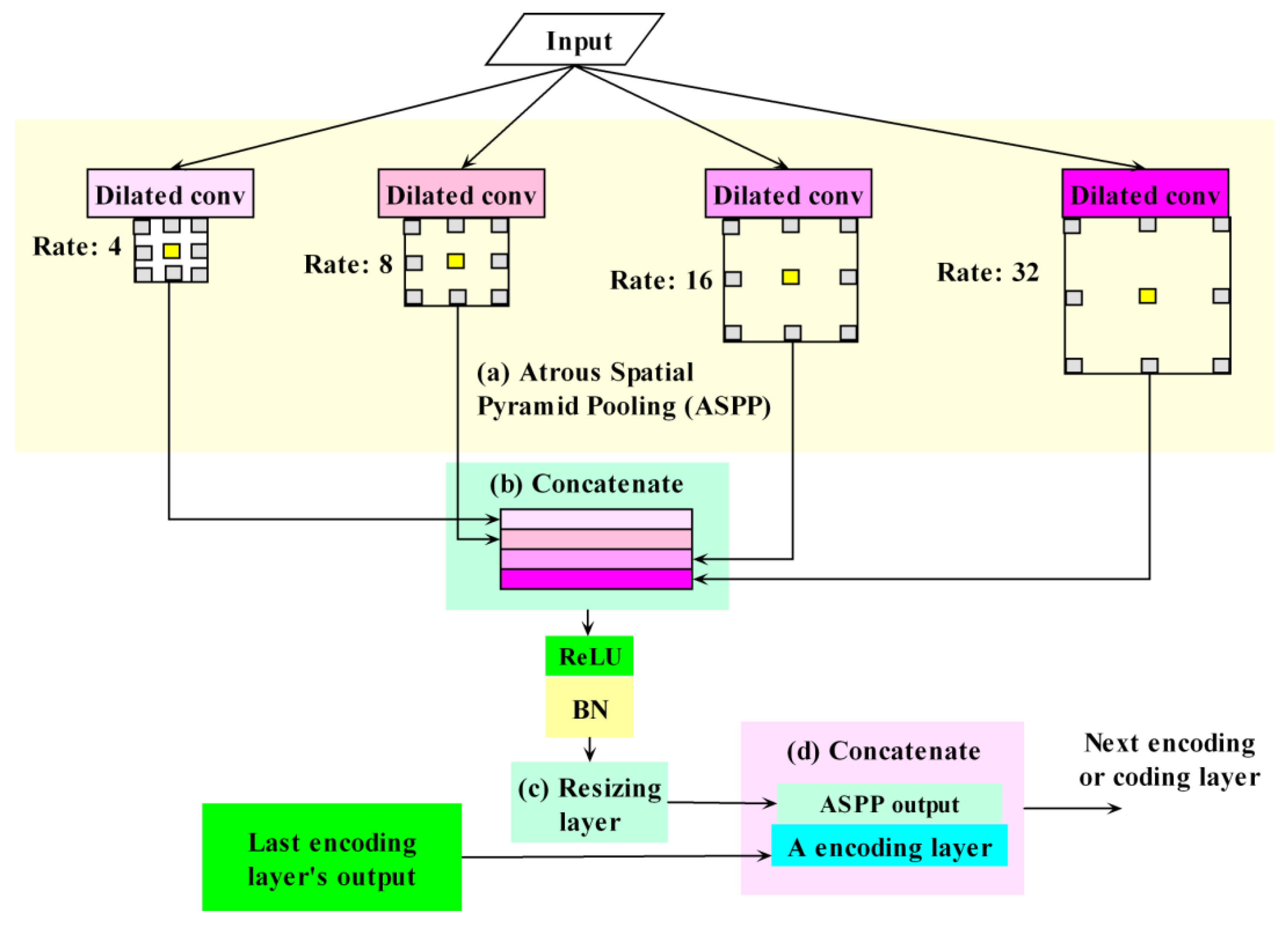
Residual learning employs skip connections or shortcuts to jump over some hidden layers to reuse activations from a previous layer until the adjacent layer learns its weights [40,41]. Residual learning can effectively reduce or avoid the problem of vanishing gradient to improve learning efficiency [42]. For convolutional neural network, a typical residual unit usually consists of two or more convolutional layers with skips that contain nonlinearities (ReLU) and batch normalization in between (Figure 2). In our previous study, residual connections have been extended between the encoding layers and the corresponding decoding layers to considerably improve the performance in the encoder-decoder-based deep neural network [38].
In the proposed architecture (Figure 1), residual connections were used in two aspects: Traditional residual units were used within each encoding or decoding layer and the extended residual connection was used between each encoding layer and its corresponding decoding layer. Similar network structure was used in our study, which showed an optimal performance [19].
Although our architecture has a U-shape structure as U-Net, it is different from U-Net. The critical difference is in skip connections that is connected by concatenation tensor operation in the U-Net but connected by residual tensor operation (matrix addition) in our architecture. Thus, the residual learning has been implemented in our network with fewer parameters than regular U-Net.

2.3. ASPP

ASPP was used to capture multi-context information to improve semantic segmentation in DeepLab Version 3+ [31]. ASPP was embedded in our network to probe convolutional feature layers with filters at multiple sampling rates, thereby capturing image context at multiple scales [43].
In our model, we set up multiple ASPP modules (Figure 1a) for the encoding and coding layers (Figure 3)—an ASPP module (Figure 3a) for each encoding or coding layer. For example, in the example architecture of Figure 1, we have five encoding layers and one coding layer, so we have six ASPP modules in total. For each ASPP module, we used four different atrous rates (r = [4,8,16,32]) to capture the objects of different sizes. Depending on complexity of the segmentation target, more atrous rates can be used in an ASPP module to capture multi-scale context information.
In each ASPP module, these dilated convolutional layers filtered using different atrous rates, were concatenated first along the channel dimension to become a matrix tensor (Figure 3b), which was then connected with the layers of ReLU activation and batch normalization (BN). To embed ASPP modules in our model, the output of the merged ASPP modules was concatenated with the corresponding encoding layer along the channel dimension to a matrix tensor as the input for next encoding or coding layer (Figure 3c,d). We also developed a custom resizing layer (Figure 3c) to alter the output shape of the merged ASPP multi-scale output to match the output shape of the corresponding encoding or coding layer to be connected. Therefore, our method implemented multi-scale ASPP modules in the network, similar to [19].

2.4. Regularizer of the Shape Representation Autoencoder

To code the morphological feature of buildings, we developed a shape representation autoencoder (Figure 4). The autoencoder has the ground truth masks of the training samples as both the input and the output to learn the shape representation. We used a structure of autoencoder similar to U-Net in Figure 1 but no residual units and ASPP modules were used and the input and the output were the same. Residual connections between each encoding layer and its corresponding decoding counterpart (but no residual units used) were used to optimize the learning process. The middle layer of latent representation was used to encode the shape characteristics of buildings, and then the input image (the building mask image) was reconstructed in the decoder based on the latent shape representation layer.
The shape representation autoencoder was pre-trained using the mask labels of the training samples and then the trained shape representation was embedded into the loss function of the semantic segmentation network as a regularizer. For binary classification, one channel of integer label can be used as the mask labels (1 represents building and 0 represents the background); for multi-classification, the K channels (K: the number of classes) of one-hot encoding [44] can be used as the mask labels. The mask labels from the data samples were used as the input and output of the shape representation autoencoder. However, pre-training is not limited to the data sample of the study area. If the mask labels from the other sources are available, we can also use them to re-train the shape autoencoder to enhance the generalization in extraction of shape representation of the buildings.

2.5. Loss Function, Multi-Scale and Boundary Effects

The total loss function (Figure 5) consists of three parts, i.e., semantic segmentation, shape and reconstruction:
t ( Y , Y ) = s e g ( Y , Y ) + λ 1 s h p ( E ( Y ) ,   E ( Y ) ) + λ 2 r e c ( Y , D ( E ( Y ) ) )
where Y denotes the ground truth mask matrix, Y’ denotes the predicted probability matrix, t represents the total loss, s e g is the primary loss of semantic segmentation, s h p is the loss of shape representation of Y, r e c is the loss of reconstruction, λ 1 and λ 2 are the weights for s h p and r e c respectively, s h p and r e c are used as regularizers in the total loss function. E(…) and D(…) represents the encoder and decoder parts in the shape representation model respectively (Figure 4).
For the loss of semantic segmentation, we used the summation of binary cross-entropy and normalized Jaccard Index that proved reliable [19]. For the reconstruction loss of the shape representation model, we used a similar combinational function (binary cross-entropy + normalized Jaccard Index); for the loss of latent shape representation, we used the mean squared error (MSE). As the hyper-parameters, an optimal solution of λ 1 and λ 2 was retrieved using grid search [45].
Introduction of multiple scales generally improves semantic segmentation in practical applications [46]. Our previous study [19] embedded the multi-scale modules connecting to the input layer to improve semantic segmentation. However, the multi-modules are limited by the input sample size. The limitations of GPU memory prevent us from using large-size inputs. Thus, in addition to the multi-scale ASPP, we used multi-scale ensemble base models to further improve the effectiveness of semantic segmentation. For a specific study area, sensitivity analysis was conducted to find an optimal number of multi-scale models. Thus, we trained a certain number of models of residual deep network with ASPP embedded and the regularizer of shape representation model, and then obtained the averages of the predicted probabilities from three models as the final predictions.
In order to make predictions, we needed to crop small patches of the same size as the input sample from a big new image, and then merge the prediction masks of each small patch together to obtain the label prediction of the entire image. This patching strategy usually leads to square structure in the edge of the resulted images and the prediction quality is decreasing when moving from the patch center [47]. Thus, we filtered out local boundary square effects of the predictions by removal of the boundaries with a distance of 16 pixels to each side (Figure 5). The same distance was used in [47] to solve the square structure. The sensitivity analysis showed that such a distance was appropriate for our study region, where the building size is small and the morphology complexity is low.
In terms of implementation, we developed the proposed method and conducted the test based on the Keras (Version: 2.2.2) with Tensorflow (Version: 1.9.0) as the backend.

3. Experimental Datasets and Evaluation

3.1. Study Region

The study region is the Dachangshan Island, a county of China, located in the southeast of Liaodong Peninsula and in the north of Changshan Islands. It is the seat of Changhai County Government in Liaoning Province, with a land area of 31.79 square kilometers, a coastline of 94.4 kilometers, and a sea area of 651.5 square kilometers. We obtained an RGB image covering the whole island (Figure 6) in April of 2019 from Google Earth (https://www.google.com/earth) with a spatial resolution of approximately 1 × 1 m2 (total pixel size: 49920 × 131840 = 6,581,452,800). Through manual interpretation, we obtained the ground truth masks of the buildings in this study region.
To improve generalization of the trained model, we used a third-part dataset (20 images) with similar bands to pre-train the models to quantify the initial parameters before training. We used a set of very-high-resolution (0.61 × 0.61 m2) images of the city of Zurich (Switzerland) (https://sites.google.com/site/michelevolpiresearch/data/zurich–dataset) by the QuickBird satellite in 2002. The original images were subset to match our base scale model with RGB channels used (near-infrared band not used). With the data, we pre-trained the models of semantic segmentation to obtain the initial coefficients (weights and bias). Then, based on the pre-trained parameters, we trained the segmentation models. Thereby, we shortened the training time.

3.2. Evaluation

The left third of the image of the study region was used for the independent test and the remaining two-thirds of the image was randomly sampled around the label features to train (60% of the samples), validate (20% of the samples) and test (20% of the samples) the models. The independent test samples were not used in training and validation, and were just used to evaluate true generalization of the model after training was finished.
For training of the models, we used the Adam with Nesterov momentum as the optimizer. We used the early stopping criterion to reduce over-fitting in training. Sensitivity analysis was also conducted to examine the effects of residual learning, the regularizer of the shape representation model and multi-scales.
To measure the performance of the trained models, we used three metrics: pixel accuracy (PA, defined as the ratio of the number of correctly classified pixels to the total number of pixels), the Jaccard index (JI, defined as the size of the intersection of two sets divided by the size of their union), and mean intersection over union (MIoU defined as the mean of JI for each class). For model comparison, in addition to MIoU and PA, we also reported three other metrics: recall (defined as the fraction of the total amount of relevant instances that were actually retrieved), precision (defined as the fraction of relevant instances among the retrieved instances) and F-measure (defined as a measure of test accuracy through the weighted average of precision and recall).
In order to validate generalization of our method, using three additional publicly accessible datasets, we conducted an extensive evaluation by comparing our method with the baseline U-Net [25], DeepLab V3+ [31], GCN [30] and residual multi-scale model [19]:
(1)
The Kaggle dataset from the Defence Science and Technology Laboratory (DSTL) Satellite Imagery Feature Detection challenge in 2017 [48]. The dataset has high-resolution panchromatic images with a 31 cm resolution, 8–band (M–band) images with a 1.24 m resolution, and shortwave infrared (A–band) images with a 7.5 m resolution (all by the WorldView–3 satellite). Panchromatic sharpening [49] was performed to fuse high-res panchromatic images and low-res images to obtain 25 images with a 31 cm resolution. We extracted binary building labels from six class labels (buildings, crops, roads, trees, vehicles and background) for semantic segmentation of buildings.
(2)
The dataset of 20 multispectral ultra-high resolution images collected by the QuickBird satellite in Zurich, Switzerland in 2002 [50]. The spatial resolution of the pan-sharpened images was 0.61 m, with 4 channels, spanning the near infrared to visible spectrum (NIR–R–G–B). We extracted binary building labels from nine class labels (road, trees, bare soil, rail, buildings, grass, water, pools and background) for semantic segmentation of buildings.
(3)
The dataset of DroneDeploy Segmentation [51], including the aerial scenes captured from drones with a ground resolution of 10 cm in 2019. The images are RGB TIFFs and the labels are PNGs with 7 colors representing 7 classes (building, clutter, vegetation, water, ground, car and background). In total, we had 36 small images (spatial resolution: 256×256) for training, 130 small images for validation, and 130 small images for testing. Due to the small number of training samples for building labels, we trained the models to perform image segmentation on all the classes (including buildings) to evaluate our model.

4. Results and Discussion

In total, we obtained approximately 0.25% of the total pixels as the label masks of the buildings. Using grid search, we got an optimal solution for the set of hyper-parameters: An initial learning rate of 0.001 with adaptive adjustment in learning, mini batch of 12 images, λ1=0.01, λ2=0.001, and 80 training epochs. The sensitivity analysis showed high learning efficiency (but no consistent change in test performance) for the pre-trained models in transfer learning using the Zurich dataset, compared with random initialization of the parameters.
In our study region of Dachangshan, the buildings were small in size and less complex in the shape and characteristics. Sensitivity analysis showed that ensemble learning of three different scale models (256 m, 512 m and 1024 m) were used to obtain an optimal solution. The results (three scales (resolutions): 4 m, 2 m and 1 m) (Table 1) for the input size of 256 × 256 show a good performance for the proposed method: For training, PA of 0.99, JI of 0.92–0.95 and MIoU of 0.91–0.94; for validation, PA of 0.98–0.99, JI of 0.89–0.92 and MIoU of 0.91–0.93; for testing, PA of 0.98–0.99, JI of 0.90–0.92 and MIoU of 0.91–0.93. For the independent test using the one-third of the study region image, the 4 m scale model obtained PA of 0.99, JI of 0.86 and MIoU of 0.82; the 2 m scale model obtained PA of 0.99, JI of 0.88 and MIoU of 0.82; the 1 m scale model obtained PA of 0.98, JI of 0.71 and MIoU of 0.82.
The results of the models with and without the regularizer of shape representation (Figure 7 for their learning curves of loss and MIoU) at three scales consistently showed better performance (lower loss and higher MIoU) for the models with the shape regularizer. Sensitivity analysis shows a 1–3% improvement of MIoU in the independent test for the models with the shape regularizer. Tong et al. (2018) [52] used a shape representation model to constrain FCN to improve multi-organ segmentation for head and neck cancers. Our results showed that the similar method consistently improved semantic segmentation of buildings using the remotely sensed data. The regularizers of shape representation helped reduce over-fitting of the trained models and improve their generalization in semantic segmentation of buildings. Although morphological features were extracted manually and used in early studies [8,9,10] to distinguish the buildings from the other geo-features, such a feature is missing in many existing studies of semantic segmentation of the buildings using deep learning. As demonstrated in the study, we used the autoencoder to extract the morphological feature as the shape representation that was embedded as the regularizer within the loss function to reduce the noise output and over-fitting. As far as we know, this is one of the first studies that fused the shape representation as the regularizer within the trained models to improve semantic segmentation of buildings.
As shown in our previous study [19], residual connections used to replace concatenation of matrix in U-Net reduced the number of parameters and thus, over-fitting. Our sensitivity analysis showed 1–3% improvement in the validation and testing by residual connections.
The scale of the input images has an important effect upon semantic segmentation given different context at different scales (resolution). To capture multi-scale contextual information, many studies embedded multi-scale modules within the models. For example, we embedded two multi-scale modules (resizing and ASPP) to capture local and long-term contextual information [19]; Zhang et al. [53] used high-resolution network to aggregate multi-scale context in segmentation of remote sensing images. Although the multi-scale module within the network can help the model to capture local and long-term or global contextual information [19,30,43,53,54], the scale of the input images may constrain the trained model from a wider or more global context. The results (Figure 8) showed that the contextual information were captured at three different scales for the input size of 256 × 256: For the scale of 4m resolution (Figure 8a,b), the input had a wider context than the other two scales; for the scale of 1m resolution (Figure 8e,f), the input had more local details than the other two scales but with less long-term or global contextual information. The trained model of each scale had different generalization in the independent test, as shown in Table 1. The model of the scale of 1m resolution had lowest Jaccard index (0.72 vs. 0.86–0.88), illustrating the importance of a long-term or global context for generalization of the trained model. However, due to the memory limitation of GPU used to train the model, there is a threshold for the size of the input image (for our case: 256). Thus, we resampled the large images to obtain the target resolution samples using the nearest neighbor interpolation. With a fixed input size, we used the resampling technique to obtain different context at three resolutions (4 m, 2 m and 1 m).
Furthermore, multi-scale (resolution) ensemble models have been used to improve generalization of the trained models. For instance, Lee (2017) [55] used the strategy of over- and under-sampling to obtain multi-scale data samples to train multiple models. The final predictions were obtained through merging the outputs of multi-scale ensemble models. This strategy can reduce the limitation of the input sample size for a single multi-scale model, and avoid the high GPU memory requirements of large multi-scale networks, although it requires more time to train multiple models.
In our method, the ASPP modules were embedded within the network to be an end-to-end integrated deep network with dynamic extraction of multi-context information based on the input. Although the input samples of a sufficient size (e.g., 1024x1024) may be expected to train a robust multi-scale model, it is actually difficult to train such a large model effectively due to the limitations of GPU memory. Generally, in order to meet the memory requirements of GPU, we may need to crop the input image or reduce the size of the input image through scaling so that our model can be trained. The use of smaller input samples by clipping in training may result in the loss of extensive context information; the use of reduced size input samples by scaling in training may result in the lack of local details. Thus, ensemble learning of multi-scale models is a compromise between a large model of a sufficient input sample size and the limitations of the available GPU memory. For this study, in addition to embedding of the multi-scale ASPP module within the model, we used the strategy of multi-scale ensemble models. In our method, the final predicted probability of building label was obtained by averaging the probability outputs (weighted by Jaccard index in the independent test) of three scale models (spatial resolution: 4 m, 2 m and 1 m). From the final prediction probability, we used the threshold of 0.5 to extract the buildings. For the ensemble predictions at the original resolution (1 m), we obtained JI of 0.81 and MIoU of 0.83, with a 1–2% improvement in MIoU compared with the results of base models, in the dependent test. Regarding the choice of model scales, for a larger study region with varying sizes of the buildings and more complex shape characteristics than ours, we may need more local and global scale models to get an optimal solution.
By comparing with the baseline U-Net, DeepLab V3+, GCN, and residual multi-scale model, our method has been extensively evaluated in independent tests (Table 2) on four data sets (DSTL, Zurich, DroneDeploy and Dachangshan). For the study region (Dachangshan) of this paper, compared with the other methods, our method improved PA, MIoU and F-measure in building semantic segmentation by 1–6%, 2–11% and 4–12%, respectively. Compared with the other methods, for the DSTL dataset, our method achieved a MIoU of 0.79 (an increase of 2–9%), a PA of 0.98 (an increase of 1–5%) and an F-measure of 0.78 (an increase of 2–8%); for the DroneDeploy dataset, our method achieved a MIoU of 0.51 (an increase of 1–12%), a PA of 0.65 (an increase of 1–6%) and an F-measure of 0.71 (an increase of 5–18%) in semantic segmentation of seven classes. For the Zurich dataset, compared with the other three methods (U-Net, DeepLab V3+ and residual autoencoder), our method achieved a MIoU of 0.91 (an increase of 2–6%) and a PA of 0.97 (an increase of 5–7%); compared with GCN, our method achieved a similar performance, with a slight lower test performance (MIoU: 0.92 vs. 0.91; PA: 0.98 vs. 0.97; F-measure: 0.96 vs. 0.95).
Compared with the baseline U-Net and DeepLab V3+, the residual multi-scale model performed better, indicating the contribution of residual learning and multi-scale modules in the network, which has been proven in an extensive comparison of our previous work [19]. As the optimal model, compared with the residual multi-scale model, our method consistently had an additional improvement in the tests of the four datasets, showing the significant contribution of the regularizer of shape representation and ensemble learning of multi-scale models.
Overall, the performance of GCN and DeepLab V3+ was similar to or better than U-Net, but similar to or worse than our method. As aforementioned, DeepLab V3+ and GCN were mainly developed for general image or video data, and their direct applications in segmentation of the buildings using remote sensing data are restricted, as shown in our test. However, some advanced techniques in DeepLab V3+ and GCN may be adapted and applied in our architecture. For example, we introduced the multi-scale modules of ASPP from DeepLab to enhance the extraction of multi-context information in our architecture (Figure 1). As a potential improvement to capture global context information, the global convolution and boundary refinement in GCN may be incorporated in our future architecture.
The results (Figure 9 for the upper left part of the test area; Figure 10 for the upper right part of the test area; Figure 11 for the lower left part of the test area) showed that the predicted output well- matched the ground truth masks of the buildings in the independent test. The majority of the ground truth masks (>80%) were basically covered by the ensemble predicted masks, illustrating the reliability of the proposed method. The ensemble results also showed fewer noise segmentations for the model with the shape regularizer, compared with that without the shape regularizer. Compared with the predictions of the model at a single scale, the ensemble predictions have the advantage of integrating the outputs from multiple base models at different scales, thus better capturing local and long-term contextual information.
There are two limitations for this study. One is a limited number of the scales in ensemble multi-scale learning. We used just three resolutions (4 m, 2 m and 1 m) to train the base models at three scales. However, our method can be conveniently generalized to more scales such as those between or beyond the three scales. This can be used to capture more local details and wider contextual information to enhance generalization in practical predictions. The other limitation is lack of post processing for the predicted masks. The post processing techniques such as conditional random fields (CRF) can be used to remove noise masks and obtain the integral results [56], but this is beyond the study scope of this paper. In the future, one important direction of the study will be the development of an integral end-to-end method fusing multiple base multi-scale models, regularizer of shape representation and post processing for semantic segmentation of the buildings.

5. Conclusions

Considering the high variability of building appearance and complex background, accurate semantic segmentation of buildings is challenging. Many deep learning methods have been developed for general or biomedical images or videos. Given the difference in spectral and morphological characteristics between remotely sensed data and general images, these methods have been only limitedly applied in semantic segmentation of buildings. In this paper, we present a residual deep learning method with incorporation of multi-scale modules, ensemble learning of multi-scale models, and the regularizer of shape representation for semantic segmentation of the buildings. Based on the encoder-decoder architecture, similar to U-Net, we used residual connections to boost learning efficiency of deep networks, and the autoencoder to encode the shape representation of the buildings as the regularizer in the model to capture the shape characteristics of the buildings to improve generalization of the trained models. To capture local and long-term or global contextual information in semantic segmentation, in addition to embedding of the multi-scale ASPP modules within the model, we applied ensemble learning of multi-scale base models to reduce the limitation in the size of the input samples. Compared with the predictions of the trained model of a single scale, the ensemble predictions improved generalization (higher MIoU). Compared with the existing representative methods (the baseline U-Net, DeepLab V3+, GCN and residual multi-scale model), our method achieved the state-of-the-art performance in the independent tests of this study region, and three additional datasets that are publicly accessible. The study showed important contributions of multi-scale residual models and ensemble learning, and regularizer of shape representation to semantic segmentation of the buildings. Although only a limited number of multi-scale models (three scale models) were used in our research case, according to the size and morphological complexity of the buildings, our flexible modeling architecture can be easily expanded by adding more scale models.
From the perspective of future model development, we consider merging global convolution and boundary refinement into the network architecture to capture global contextual information, as well as integrating multiple base multi-scale models, regularizer of shape representation and post processing into a systematic end-to-end method to improve the efficiency in learning and predicting for segmentation of the buildings.

Author Contributions

C.W. was responsible for conceptualization, methodology, data, literature of building extraction and financial support. L.L. was responsible for conceptualization, methodology, literature of deep learning, software, validation, formal analysis and writing. All authors have read and agreed to the published version of the manuscript.

Funding

This work was supported in part by the National Natural Science Foundation of China under grant number 41471376, in part by the Strategic Priority Research Program of Chinese Academy of Sciences grant number XDA19040501, and in part by the project on the Mechanism of Multi-Scale Urban Gray Scale on Thermal Landscape of Institute of Aerospace Information Innovation, Chinese Academy of Sciences.

Acknowledgments

The support of NVIDIA Corporation with the donation of the Titan Xp GPUs used for this research.

Conflicts of Interest

The authors declare no conflict of interest.

References

  1. Bischke, B.; Helber, P.; Folz, J.; Borth, D.; Dengel, A. Multi-task learning for segmentation of building footprints with deep neural networks. In Proceedings of the 2019 IEEE International Conference on Image Processing (ICIP), Taipei, Taiwan, 22–25 September 2019; pp. 1480–1484. [Google Scholar]
  2. Lin, X.; Zhang, J. Object-based morphological building index for building extractionfrom high resolution remote sensing imagery. Acta Geod. Cartogr. Sin. 2017, 46, 724–733. [Google Scholar]
  3. Yi, Y.N.; Zhang, Z.J.; Zhang, W.C.; Zhang, C.R.; Li, W.D.; Zhao, T. Semantic Segmentation of Urban Buildings from VHR Remote Sensing Imagery Using a Deep Convolutional Neural Network. Remote Sens. 2019, 11, 1774. [Google Scholar] [CrossRef] [Green Version]
  4. Wang, J.; Qin, Q.; Ye, Q.; Wang, J.; Qin, X.; Yang, X. A Survey of Building Extraction Methods from Optical High Resolution Remote Sensing Imagery. Remote Sens. Technol. Appl. 2016, 31, 653–662. [Google Scholar]
  5. Akçay, H.G.; Aksoy, S. Automatic detection of geospatial objects using multiple hierarchical segmentations. IEEE Trans. Geosci. Remote Sens. 2008, 46, 2097–2111. [Google Scholar] [CrossRef]
  6. Blaschke, T.; Hay, G.J.; Kelly, M.; Lang, S.; Hofmann, P.; Addink, E.; Feitosa, R.Q.; van der Meer, F.; van der Werff, H.; van Coillie, F.; et al. Geographic object-based image analysis—towards a new paradigm. ISPRS J. Photogramm. Remote Sens. 2014, 87, 180–191. [Google Scholar] [CrossRef] [Green Version]
  7. Tian, H.; Yang, J.; Wang, Y.; Li, G. Towards Automatic Building Extraction: Variational Level Set Model Using Prior Shape Knowledge. Acta Autom. Sin. 2010, 36, 1502–1511. [Google Scholar] [CrossRef]
  8. Huang, X.; Zhang, L. A multidirectional and multiscale morphological index for automatic building extraction from multispectral GeoEye-1 imagery. Photogramm. Eng. Remote Sens. 2011, 77, 721–732. [Google Scholar] [CrossRef]
  9. Pesaresi, M.; Gerhardinger, A.; Kayitakire, F. A robust built-up area presence index by anisotropic rotation-invariant textural measure. IEEE J. Select. Top. Appl. Earth Obser. Remote Sens. 2008, 1, 180–192. [Google Scholar] [CrossRef]
  10. Huang, X.; Zhang, L. Morphological building/shadow index for building extraction from high-resolution imagery over urban areas. IEEE J. Select. Top. Appl. Earth Obser. Remote Sens. 2011, 5, 161–172. [Google Scholar] [CrossRef]
  11. Adams, R.; Bischof, L. Seeded region growing. IEEE Trans. Pattern Anal. Mach. Intell. 1994, 16, 641–647. [Google Scholar] [CrossRef] [Green Version]
  12. Comaniciu, D.; Meer, P. Mean shift: A robust approach toward feature space analysis. IEEE Trans. Pattern Anal. Mach. Intell. 2002, 24, 603–619. [Google Scholar] [CrossRef] [Green Version]
  13. Rother, C.; Kolmogorov, V.; Blake, A. Interactive foreground extraction using iterated graph cuts. ACM Trans. Gr. 2004, 23, 3. [Google Scholar]
  14. Aytekın, Ö.; Erener, A.; Ulusoy, İ.; Düzgün, Ş. Unsupervised building detection in complex urban environments from multispectral satellite imagery. Int. J. Remote Sens. 2012, 33, 2152–2177. [Google Scholar] [CrossRef]
  15. Das, S.; Mirnalinee, T.; Varghese, K. Use of salient features for the design of a multistage framework to extract roads from high-resolution multispectral satellite images. IEEE Trans. Geosci. Remote Sens. 2011, 49, 3906–3931. [Google Scholar] [CrossRef]
  16. Song, M.; Civco, D. Road extraction using SVM and image segmentation. Photogramm. Eng. Remote Sens. 2004, 70, 1365–1371. [Google Scholar] [CrossRef] [Green Version]
  17. Wang, Y.; Song, H.; Zhang, Y. Spectral-spatial classification of hyperspectral images using joint bilateral filter and graph cut based model. Remote Sens. 2016, 8, 748. [Google Scholar] [CrossRef] [Green Version]
  18. Tian, S.; Zhang, X.; Tian, J.; Sun, Q. Random forest classification of wetland landcovers from multi-sensor data in the arid region of Xinjiang, China. Remote Sens. 2016, 8, 954. [Google Scholar] [CrossRef] [Green Version]
  19. Li, L.F. Deep Residual Autoencoder with Multiscaling for Semantic Segmentation of Land-Use Images. Remote Sens. 2019, 11, 2142. [Google Scholar] [CrossRef] [Green Version]
  20. LeCun, Y.; Bengio, Y.; Hinton, G. Deep learning. Nature 2015, 521, 436–444. [Google Scholar] [CrossRef]
  21. Zhang, L.P.; Zhang, L.F.; Du, B. Deep Learning for Remote Sensing Data A technical tutorial on the state of the art. IEEE Geosci. Remote Sens. Mag. 2016, 4, 22–40. [Google Scholar] [CrossRef]
  22. Zhu, X.X.; Tuia, D.; Mou, L.C.; Xia, G.S.; Zhang, L.P.; Xu, F.; Fraundorfer, F. Deep Learning in Remote Sensing. IEEE Geosci. Remote Sens. Mag. 2017, 5, 8–36. [Google Scholar] [CrossRef] [Green Version]
  23. Long, J.; Shelhamer, E.; Darrell, T. Fully convolutional networks for semantic segmentation. In Proceedings of the IEEE Conference on Computer Vision and Pattern Recognition (CVRP), Boston, MA, USA, 7–12 June 2015; pp. 3431–3440. [Google Scholar]
  24. Yu, H.S.; Yang, Z.G.; Tan, L.; Wang, Y.N.; Sun, W.; Sun, M.G.; Tang, Y.D. Methods and datasets on semantic segmentation: A review. Neurocomputing 2018, 304, 82–103. [Google Scholar] [CrossRef]
  25. Ronneberger, O.; Fischer, P.; Brox, T. U-Net: Convolutional Networks for Biomedical Image Segmentation. arXiv 2015, arXiv:1505.04597. [Google Scholar]
  26. Badrinarayanan, V.; Kendall, A.; Cipolla, R. Segnet: A deep convolutional encoder-decoder architecture for image segmentation. IEEE Trans. Pattern Anal. Mach. Intell. 2017, 39, 2481–2495. [Google Scholar] [CrossRef]
  27. Chen, L.-C.; Papandreou, G.; Kokkinos, I.; Murphy, K.; Yuille, A.L. Semantic image segmentation with deep convolutional nets and fully connected CRFs. arXiv 2014, arXiv:14127062. [Google Scholar]
  28. Chen, L.-C.; Papandreou, G.; Kokkinos, I.; Murphy, K.; Yuille, A.L. DeepLab: Semantic image segmentation with deep convolutional nets, atrous convolution, and fully connected CRFs. IEEE Trans. Pattern Anal. Mach. Intell. 2017, 40, 834–848. [Google Scholar] [CrossRef]
  29. Lin, G.; Milan, A.; Shen, C.; Reid, I. Refinenet: Multi-path refinement networks for high-resolution semantic segmentation. In Proceedings of the IEEE Conference on Computer Vision and Pattern Recognition, Honolulu, HI, USA, 21–26 July 2017; pp. 1925–1934. [Google Scholar]
  30. Peng, C.; Zhang, X.; Yu, G.; Luo, G.; Sun, J. Large Kernel Matters—Improve Semantic Segmentation by Global Convolutional Network. In Proceedings of the IEEE Conference on Computer Vision and Pattern Recognition, Honolulu, HI, USA, 21–26 July 2017; pp. 4353–4361. [Google Scholar]
  31. Chen, L.-C.; Zhu, Y.; Papandreou, G.; Schroff, F.; Adam, H. Encoder-decoder with atrous separable convolution for semantic image segmentation. In Proceedings of the European Conference on Computer Vision (ECCV), Munich, Germany, 8–14 September 2018; pp. 801–818. [Google Scholar]
  32. Zuo, T. Research of Building Extraction Technology for High-Resolution Remote Sensing Images; University of Science and Technology of China: Hefei, China, 2017. (In Chinese) [Google Scholar]
  33. Maggiori, E.; Tarabalka, Y.; Charpiat, G.; Alliez, P. Convolutional neural networks for large-scale remote-sensing image classification. IEEE Trans. Geosci. Remote Sens. 2016, 55, 645–657. [Google Scholar] [CrossRef] [Green Version]
  34. Yang, J.; Mei, T.; Zhong, S. Application of Convolutional Neural Netowrk using region information to remote sensing image classification. Comput. Eng. Appl. 2018, 54, 188–195. [Google Scholar]
  35. Qin, Y.; Wu, Y.; Li, B.; Gao, S.; Liu, M.; Zhan, Y. Semantic Segmentation of Building Roof in Dense Urban Environment with Deep Convolutional Neural Network: A Case Study Using GF2 VHR Imagery in China. Sensors 2019, 19, 1164. [Google Scholar] [CrossRef] [Green Version]
  36. Shi, Y.; Li, Q.; Zhu, X.X. Building segmentation through a gated graph convolutional neural network with deep structured feature embedding. ISPRS J. Photogramm. 2020, 159, 184–197. [Google Scholar] [CrossRef]
  37. Ge, Y.; Jin, Y.; Stein, A.; Chen, Y.; Wang, J.; Wang, J.; Cheng, Q.; Bai, H.; Liu, M.; Atkinson, P.M. Principles and methods of scaling geospatial Earth science data. Earth Sci. Rev. 2019, 197, 102897. [Google Scholar] [CrossRef]
  38. Li, L.; Fang, Y.; Wu, J.; Wang, C.; Ge, Y. Encoder-Decoder Full Residual Deep Networks for Robust Regression and Spatiotemporal Estimation. IEEE Trans. Nerual Netw. Learn. Syst. 2020. [Google Scholar] [CrossRef] [PubMed]
  39. Garcia-Garcia, A.; Orts-Escolano, S.; Oprea, S.; Villena-Martinez, V.; Garcia-Rodriguez, J. A review on deep learning techniques applied to semantic segmentation. arXiv 2017, arXiv:170406857. [Google Scholar]
  40. He, K.M.; Zhang, X.Y.; Ren, S.Q.; Sun, J. Deep Residual Learning for Image Recognition. In Proceedings of the IEEE Conference on Computer Vision and Pattern Recognition, Las Vegas, NV, USA, 27–30 June 2016; pp. 770–778. [Google Scholar]
  41. He, K.M.; Zhang, X.Y.; Ren, S.Q.; Sun, J. Identity Mappings in Deep Residual Networks. In Lecture Notes in Computer Science; Springer: Cham, Switzerland, 2016; Volume 9908, pp. 630–645. [Google Scholar]
  42. Wiki, Residual Neural Network. 2020. Available online: https://en.wikipedia.org/wiki/Residual_neural_network (accessed on 1 April 2020).
  43. Chen, L.-C.; Papandreou, G.; Schroff, F.; Adam, H. Rethinking atrous convolution for semantic image segmentation. arXiv 2017, arXiv:170605587. [Google Scholar]
  44. Sethi, A. One-Hot Encoding vs. Label Encoding using Scikit-Learn. 2020. Available online: https://www.analyticsvidhya.com/blog/2020/03/one-hot-encoding-vs-label-encoding-using-scikit-learn (accessed on 1 February 2020).
  45. Bergstra, J.; Bengio, Y. Random Search for Hyper-Parameter Optimization. Mach. Learn. Res. 2012, 13, 281–305. [Google Scholar]
  46. Cui, W.; Wang, F.; He, X.; Zhang, D.; Xu, X.; Yao, M.; Wang, Z.; Huang, J. Multi-Scale Semantic Segmentation and Spatial Relationship Recognition of Remote Sensing Images Based on an Attention Model. Remote Sens. 2019, 11, 1044. [Google Scholar] [CrossRef] [Green Version]
  47. Iglovikov, V.; Mushinskiy, S.; Osin, V. Satellite imagery feature detection using deep convolutional neural network: A kaggle competition. arXiv 2017, arXiv:170606169. [Google Scholar]
  48. Dstl Satellite Imagery Feature Detection. Available online: https://www.kaggle.com/c/dstl-satellite-imagery-feature-detection (accessed on 10 January 2020).
  49. Padwick, C.; Deskevich, M.; Pacifici, F.; Smallwood, S. WorldView-2 pan-sharpening. In Proceedings of the American Society for Photogrammetry and Remote Sensing Annual Conference, San Diego, CA, USA, 26–30 April 2010. [Google Scholar]
  50. Volpi, M.; Ferrari, V. Semantic segmentation of urban scenes by learning local class interactions. In Proceedings of the IEEE Conference on Computer Vision and Pattern Recognition (CVPR), Workshops. Looking from Above: When Earth Observation Meets Vision (EARTHVISION), Boston, MA, USA, 7–12 June 2015; pp. 1–9. [Google Scholar]
  51. Aburas, M.M.; Ho, Y.M.; Ramli, M.F.; Ash’aari, Z.H. The simulation and prediction of spatio-temporal urban growth trends using cellular automata models: A review. Int. J. Appl. Earth Obs. Geoinf. 2016, 52, 380–389. [Google Scholar] [CrossRef]
  52. Tong, N.; Gou, S.; Yang, S.; Ruan, D.; Sheng, K. Fully automatic multi-organ segmentation for head and neck cancer radiotherapy using shape representation model constrained fully convolutional neural networks. Med. Phys. 2018, 45, 4558–4567. [Google Scholar] [CrossRef] [Green Version]
  53. Zhang, J.; Lin, S.; Ding, L.; Bruzzone, L. Multi-Scale Context Aggregation for Semantic Segmentation of Remote Sensing Images. Remote Sens. 2020, 12, 701. [Google Scholar] [CrossRef] [Green Version]
  54. Lin, D.; Ji, Y.; Lischinski, D.; Cohen-Or, D.; Huang, H. Multi-scale context intertwining for semantic segmentation. In Proceedings of the European Conference on Computer Vision (ECCV), Munich, Germany, 8–14 September 2018; pp. 603–619. [Google Scholar]
  55. Kaggle Team. Dstl Satellite Imagery Competition, 1st Place Winner’s Interview: Kyle Lee. 2018. Available online: https://medium.com/kaggle-blog/dstl-satellite-imagery-competition-1st-place-winners-interview-kyle-lee-6571ce640253 (accessed on 10 November 2019).
  56. Hoberg, T.; Rottensteiner, F.; Feitosa, R.Q.; Heipke, C. Conditional random fields for multitemporal and multiscale classification of optical satellite imagery. IEEE Trans. Geosci. Remote Sens. 2014, 53, 659–673. [Google Scholar] [CrossRef]
Figure 1. The architecture based on the encoder-decoder U-Net structure with fusion of residual connections, multi-scale ASPP (atrous spatial pyramid pooling) modules and shape regularizer.
Remotesensing 12 02932 g001
Figure 2. A residual unit (two convolutional layers, each following an activation layer and a batch normalization layer).
Remotesensing 12 02932 g002
Figure 3. An ASPP module for embedding in the segmentation model.
Remotesensing 12 02932 g003
Figure 4. The autoencoder of shape representation model for buildings.
Remotesensing 12 02932 g004
Figure 5. Training (a) of the base segmentation model with incorporation of shape representation regularizer and prediction (b) by multi-scale trained models.
Remotesensing 12 02932 g005
Figure 6. The study region of Dachangshan Island of China with a RGB image.
Remotesensing 12 02932 g006
Figure 7. Learning curves of loss and MIoU of the models with and without the shape regularizer at different scales. (a) 4 m resolution validation loss, (b) 4 m resolution validation MIoU, (c) 2 m resolution validation loss, (d) 2 m resolution validation MIoU, (e) 1 m resolution validation loss, (f) 1 m resolution validation MIoU.
Remotesensing 12 02932 g007
Figure 8. Comparison of original RGB images, ground truth masks and predicted masks at three spatial scales.
Remotesensing 12 02932 g008
Figure 9. Ground truth mask (a) vs. predicted mask (b) of the buildings for the upper left part of the test area.
Remotesensing 12 02932 g009
Figure 10. Ground truth mask (a) vs. predicted mask (b) of the buildings for the upper right part of the test area.
Remotesensing 12 02932 g010
Figure 11. Ground truth mask (a) vs. predicted mask (b) of the buildings for the lower left part of the test area.
Remotesensing 12 02932 g011
Table 1. Metrics of training, validation, testing, and independent test at three scales.
Scale (Resolution) MetricTrainingValidationTesting Independent Test
4m Number of Samples 4595153115312245
PA0.990.990.990.99
JI0.920.920.910.86
MIoU 0.940.930.930.82
2m Number of Samples 7531251025109464
PA0.990.980.980.99
JI0.940.920.920.88
MIoU 0.930.930.930.82
1m Number of Samples 75402513251343,708
PA0.990.980.980.99
JI0.950.890.900.71
MIoU 0.910.910.910.82
Table 2. Comparison of the results of the independent tests on four datasets (DSTL, Zurich, DroneDeploy and Dachangshan) and five methods.
Target Class, Sample Size, Model and MetricsDSTLZurichDroneDeploy Dachangshan
Target Class Building Building All Classes bBuilding
Size of training samples 24261932364595
U-NetMIoU0.720.860.410.77
PA0.950.900.590.95
Recall 0.690.900.650.79
Precision 0.780.890.450.80
F-measure0.730.900.530.80
DeepLab V3+MIoU0.700.850.420.76
PA0.930.920.640.88
Recall 0.660.910.630.79
Precision 0.750.920.640.73
F-measure0.700.920.630.75
Global CNNMIoU0.770.920.390.82
PA0.970.980.630.97
Recall 0.720.960.750.86
Precision 0.810.930.450.81
F-measure0.760.960.560.83
Residual Autoencoder aMIoU0.750.890.500.80
PA0.960.920.610.97
Recall 0.690.950.810.83
Precision 0.790.970.560.84
F-measure0.74 0.960.660.83
Residual multi-scale model with shape regularizer MIoU0.79c0.910.510.83
PA0.980.970.650.99
Recall 0.730.950.860.87
Precision 0.840.940.610.87
F-measure0.780.950.710.87
a: No use of the shape regularizer; b: All the classes including building, clutter, vegetation, water, ground, car, and the background; c: the bold number indicates the best metric value (MIoU or F-measure) across different methods for each dataset.

