Advancing the Mapping of Mangrove Forests at National-Scale Using Sentinel-1 and Sentinel-2 Time-Series Data with Google Earth Engine: A Case Study in China

Abstract

A high resolution mangrove map (e.g., 10-m), including mangrove patches with small size, is urgently needed for mangrove protection and ecosystem function estimation, because more small mangrove patches have disappeared with influence of human disturbance and sea-level rise. However, recent national-scale mangrove forest maps are mainly derived from 30-m Landsat imagery, and their spatial resolution is relatively coarse to accurately characterize the extent of mangroves, especially those with small size. Now, Sentinel imagery with 10-m resolution provides an opportunity for generating high-resolution mangrove maps containing these small mangrove patches. Here, we used spectral/backscatter-temporal variability metrics (quantiles) derived from Sentinel-1 SAR (Synthetic Aperture Radar) and/or Sentinel-2 MSI (Multispectral Instrument) time-series imagery as input features of random forest to classify mangroves in China. We found that Sentinel-2 (F1-Score of 0.895) is more effective than Sentinel-1 (F1-score of 0.88) in mangrove extraction, and a combination of SAR and MSI imagery can get the best accuracy (F1-score of 0.94). The 10-m mangrove map was derived by combining SAR and MSI data, which identified 20003 ha mangroves in China, and the area of small mangrove patches (<1 ha) is 1741 ha, occupying 8.7% of the whole mangrove area. At the province level, Guangdong has the largest area (819 ha) of small mangrove patches, and in Fujian, the percentage of small mangrove patches is the highest (11.4%). A comparison with existing 30-m mangrove products showed noticeable disagreement, indicating the necessity for generating mangrove extent product with 10-m resolution. This study demonstrates the significant potential of using Sentinel-1 and Sentinel-2 images to produce an accurate and high-resolution mangrove forest map with Google Earth Engine (GEE). The mangrove forest map is expected to provide critical information to conservation managers, scientists, and other stakeholders in monitoring the dynamics of the mangrove forest.

1. Introduction

Mangrove forest ecosystems, which are a major component of coastal and estuarine zones in tropical and subtropical regions, provide substantial socio-economic functions, such as supplying nutrients and grounds for fish and shellfish, and producing wood and non-wood goods [1,2,3]. In addition, mangrove forests also provide important environmental functions [4,5,6,7,8]. For example, mangrove forests play a crucial role in the global carbon cycle [9,10,11,12,13]. Previous studies have found that mangrove forests are one of the most carbon-rich ecosystems, and their average total carbon storage at a specified area unit is five times larger than that of tropical terrestrial, temperate, and boreal forests [6]. Information about the spatial distribution and extent of mangroves is a central component to quantitatively estimate their ecosystem service value [14]. Recent studies have shown that, over the past two decades, global mangrove forests have been declining rapidly and are gradually fragmenting into small patches. This can be attributed to anthropogenic activities, such as aquaculture and land reclamation [15,16,17,18]. If the loss continues at the present rate, mangroves are expected to be extinct within the next 100 years [19,20]. As a result, there is an urgent need for advancing the monitoring capabilities of mangrove forests to prevent the extinction of mangroves and assess changes in mangrove ecosystem functions.

Remote sensing imagery is ideal to monitor the spatial distribution and extent of land cover [21], but applying this to monitoring large-scale mangroves is challenging, due to the widespread existence of scattered mangrove trees, which are generally mixed with other types of plants (e.g., salt marsh), and the increasing number of small mangrove patches caused by human destruction and new mangrove plantation. Although high-resolution (<1 m) imagery (e.g., Worldview, Quickbird, and aerial photographs) can be used to identify individual mangrove trees, large-scale mangrove mapping based on these data is limited by cost, data availability, and volume. Consequently, freely available satellite imagery (e.g., Landsat) with moderate resolution ($\ge 30 \mathrm{m}$) is widely used to extract large-scale mangrove forests. For example, Chen et al. (2017) [22] mapped mangrove forest extent in China from 2015 based on 30-m Landsat imagery; the Global Mangrove Watch (GMW) [23] applied ALOS PALSAR/JERS-1 (25 m) and Landsat (30 m) imagery to produce global mangrove forest maps from 1996 to 2010.

However, these products with spatial resolutions larger than 30 m are relatively coarse for accurately characterizing the distribution of mangrove forests [23]. For example, due to new mangrove growth and damage caused by human beings, there are many mangrove patches smaller than the minimum discriminating area of these products [23,24,25].

Approaches for remote sensing-based mangrove mapping can be grouped into two categories. One is using single-date imagery, and the other is using multi-temporal imagery. The first approach mainly adopts single-date optical, SAR (synthetic aperture radar), or a combination of these two types of imagery. The single-date imagery is difficult to be applied in large-scale mangrove mapping because it is hard to guarantee that all clear images covered study area are obtained at low tide, a period during which the canopy of mangrove is not inundated by water and, hence, can be identified [26]. Additionally, the spectral similarity between mangroves and other land cover types (such as natural terrestrial forests) also makes it more difficult to accurately identify mangroves in single-date imagery [27]. Compared to using single-date imagery, using time-series imagery can separate mangrove forests from other land cover types at large scales, since the temporal profile of the spectrum for mangroves is distinctive with influence of tidal variability. For example, for mangroves, the spectral reflectance of near infrared (NIR) and short wave infrared (SWIR) obtained at high tide declines abruptly compared to that obtained at low tide. Spectral-temporal features (such as quantiles) derived from the time-series of remote sensing imagery are usually adopted to delineate spectrum temporal profiles and are applied to extract mangroves. For example, Hu et al. (2018) [27] applied spectral-temporal features derived from Landsat time-series imagery to monitor mangrove forests in China. However, most of studies used optical imagery, and only a few studies adopted SAR data. For example, Chen et al. (2017) [22] used information about yearlong and fresh water bodies derived from Sentinel-1 time-series data (2014–2016) to identify mangrove forests, which are periodically inundated with water with the influence of tidal dynamics.

Since 2014, the constellations of Sentinel-1A & 1B and Sentinel-2A & 2B were successively launched [28]. Sentinel-1 C-band SAR data are insensitive to clouds and may be useful to monitor mangrove forests, which are distributed in regions that are often cloudy. Sentinel-2 MSI (Multispectral Instrument) imagery has 13 spectral bands, including four red edge bands sensitive to biophysical features (e.g., leaf chlorophyll and water content) of vegetation, with a spatial resolution of 10 m and temporal resolution of 5 days. Compared to Landsat imagery (7/8 bands, 30 m, 8/16 days), which is commonly used in large-scale mangrove extraction, Sentinel-2 has a clear improvement in spatial and temporal resolution [29]. Therefore, Sentinel-1 and Sentinel-2 imagery, which are freely available, may have the potential to advance the mapping of mangrove forests. In addition, Sentinel data can also be processed through the Google Earth Engine (GEE) cloud computing platform, which facilitates challenges related to massive data volumes processed in large-area mapping. Several studies have been conducted for mangrove mapping at a regional scale using Sentinel imagery. For example, Chen et al. (2017) [30] identified the mangrove forests in Dongzhaigang, China, with the use of Sentinel-2 imagery; Manna et al. (2018) [31] mapped mangroves in Sundarban based on Sentinel-2 imagery. Nevertheless, no research has been reported for using time-series Sentinel-1 and Sentinel-2 data to produce national-scale mangrove maps.

Therefore, our study applied Sentinel imagery on the Google Earth Engine platform to generate a national-scale mangrove forest map, and further explored how a 10-m mangrove map derived from Sentinel imagery can improve our knowledge of mangroves on existing 30-m products generated from Landsat imagery. Our study focused on the coastal zones of China, whose mangrove ecosystems have a scattered distribution and are mixed with salt marsh. Besides, in China, the number of small mangrove patches is increasing due to anthropogenic activities, such as destruction and successive planting in large areas [32]. Several studies have evaluated the spatial distribution and extent of mangrove forests in China based on Landsat imagery with 30-m resolution. However, the actual extent and area of mangroves containing those small mangrove patches is still unclear because these small patches are smaller than the minimum discriminating area (1 ha) of Landsat imagery.

In summary, the objectives of this study are: (1) generate a national-scale mangrove forests map with 10-m resolution in China using Sentinel-1 and Sentinel-2 time-series imagery; (2) explore an optimal combination of features from Sentinel-1 and Sentinel-2 time-series imagery for large-scale mangrove extraction, which has the potential to be transferred globally; (3) quantitatively and qualitatively compare the difference between the 10-m mangrove forest map and existing available products.

2. Materials

2.1. Study Area

Our study area covers all potential areas that allow for the growth of mangroves: the provinces of Hainan, Guangdong, Fujian, Zhejiang and Taiwan, the Guangxi Zhuang Autonomous Region, Hong Kong Special Administrative Region, and the Macao Special Administrative Region. The geographical range is from 18°N to 30°N and from 105°E to 125°E (Figure 1). Within that area, the southern and northern boundaries of the natural mangrove forest are Sanya (Hainan Province) at 18°09′N and Fuding (Fujian Province) at 27°20′N, while the planted mangrove forest can extend to Leqing (Zhejiang Province) at 28°25′N. The climate of our study area is tropical and subtropical with a mean annual temperature of 22.31 °C and a mean annual rainfall of 1677 mm [33]. In addition, there are various types of tides, including irregular diurnal (dominant on the east coasts of Hainan, and west coasts of Taiwan), irregular semi-diurnal (dominant on the south coasts of Guangdong, and the southwest and east coasts of Taiwan), regular diurnal (dominant on the coasts of Guangxi, and west coasts of Guangdong and Hainan), and regular semi-diurnal (dominant on the coasts of Fujian) [32].

2.2. Data

In this study, Sentinel imagery was sourced, accessed, and processed based on GEE, a cloud-based platform for analyzing planetary-scale environmental data, such as satellite imagery. Additionally, ancillary data (e.g., elevation) were also used.

2.2.1. Sentinel-1 Imagery

The Sentinel-1 mission comprises two polar-orbiting satellites, carrying a single C-band SAR instrument at a central frequency of 5.405 GHz. These two satellites enable them to acquire data at a time interval of 6 days in specific regions and in four modes: stripmap (SM), Interferometric Wide swath (IW), Extra-Wide swath (EW), and Wave mode (WV) [22,34].

In our study, we used the Sentinel-1 SAR Ground Range Detected (GRD) product, which has two backscatter bands (dual-polarization of vertical transmitting with horizontal receiving (VH) bands and vertical transmitting with vertical receiving (VV) (

Table 1. The central frequency and spatial resolution for Sentinel-1 bands used in this study. VV represents vertical transmitting with vertical receiving and VH represents vertical transmitting with horizontal receiving.

Band	Central Frequency (GHz)	Spatial Resolution (m)
VV	5.405	10
VH

)) and high geometric accuracy in the default IW mode. The GRD product was processed with the Sentinel-1 Toolbox in the following steps: (1) thermal noise removal; (2) radiometric calibration to get the backscatter intensity; (3) terrain correction based on Shuttle Radar Topography Mission (SRTM) or Advanced Spaceborne Thermal Emission and Reflection Radiometer (ASTER) data; (4) data conversion from terrain-corrected backscatter coefficient (${\sigma }^0$) to decibels (dB) [22,34]. Finally, we acquired a total of 6179 Sentinel-1A images from 23 June 2015, to 21 October 2018, and the spatial distribution of the total observation number for each pixel is presented in Figure 1a.

2.2.2. Sentinel-2 Imagery

The Sentinel-2 mission also includes two satellites, which enable a revisit time of 5 days. The instrument carried on Sentinel-2 is called MSI, which can acquire 13 spectral bands at variable spatial resolution (10 m, 20 m, 60 m) [29].

Our study mainly adopted Sentinel-2 imagery (Level 1C Top-of Atmosphere reflectance products) with 10 m and 20 m resolution acquired from the same period as Sentinel-1, as mentioned in Section 2.2.1. The reason why we did not adopt the rest of bands in Sentinel-2 imagery is that the spatial resolution of these bands is 60 m. The details of these imagery are listed in

Table 2. The central wavelength and spatial resolution for Sentinel-2 bands used in this study. NIR represents near infrared and SWIR represents short wave infrared.

Band	Abbreviation	Central Wavelength (nm)	Spatial Resolution (m)
2 blue	B2	490	10
3 green	B3	560	10
4 red	B4	665	10
5 red edge 1	B5	705	20
6 red edge 2	B6	740	20
7 red edge 3	B7	783	20
8 NIR	B8	842	10
8A red edge 4	B8A	865	20
11 SWIR 1	B11	1610	20
12 SWIR 2	B12	2190	20

. A total of 22371 Sentinel-2 images were used in our study, and the spatial distribution of the number of good observations is presented in Figure 1b.

2.2.3. Other Auxiliary Data

To separate mangroves from other land cover types, we used the Shuttle Radar Topography Mission (SRTM) elevation data with 30 m resolution in the GEE data pool [35].

Global coastline data, derived from the open Street Map Data [36], were used to exclude areas where mangroves are not distributed through generating a 10 km buffer zone along the coastline.

3. Methods

3.1. Preprocessing

3.1.1. Cloud Mask

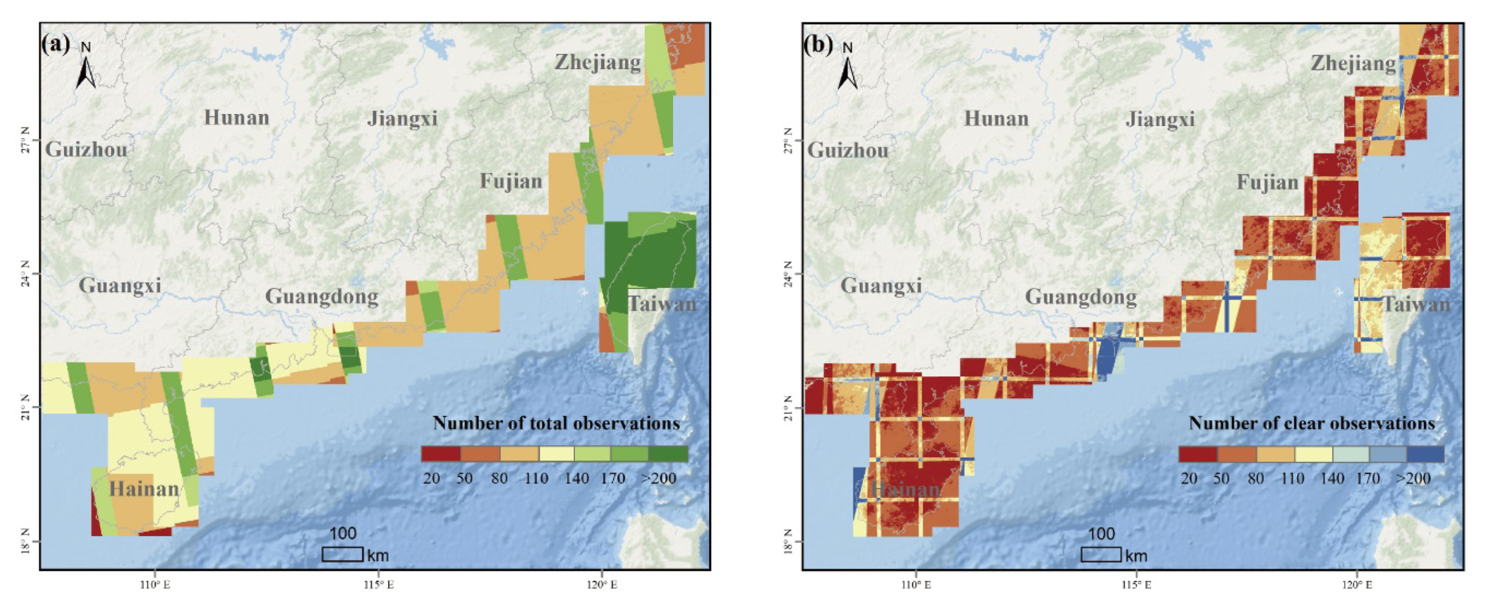
Sentinel-2 MSI imagery is easily contaminated by clouds, especially in tropical and subtropical regions where mangrove forests grow. The Level-1 product of Sentinel-2 provides a Quality Assessment (QA) band that labels cloud and cirrus pixels. By using this band, we discriminated and removed cloud and cirrus pixels from each image.

3.1.2. Spectral Indices Calculation

Spectral indices enhance the spectral properties of vegetation and water. Here, we adopted the seven spectral indices listed in

Table 3. Vegetation indices (VI) derived from Sentinel-2 imagery. $\rho$ stands for Top-of Atmosphere reflectance at a specified wavelength.

Vegetation Indices	Abbreviation	Equations	Reference
Normalized Difference Vegetation Index	NDVI	$\frac{{\rho }_{842\mathrm{nm}}-{\rho }_{665\mathrm{nm}}}{{\rho }_{842\mathrm{nm}}+{\rho }_{665\mathrm{nm}}}$	[37]
Normalized Difference Water Index	NDWI	$\frac{{\rho }_{842\mathrm{nm}}-{\rho }_{1610\mathrm{nm}}}{{\rho }_{842\mathrm{nm}}+{\rho }_{1610\mathrm{nm}}}$	[38]
Modified Normalized Difference Water Index	MNDWI	$\frac{{\rho }_{560\mathrm{nm}}-{\rho }_{1610\mathrm{nm}}}{{\rho }_{560\mathrm{nm}}+{\rho }_{1610\mathrm{nm}}}$	[39]
Plant Senescence Reflectance Index 1	${\mathrm{PSRI}}_1$	$\frac{{\rho }_{665\mathrm{nm}}-{\rho }_{490\mathrm{nm}}}{{\rho }_{705\mathrm{nm}}}$	[40]
Plant Senescence Reflectance Index 2	${\mathrm{PSRI}}_2$	$\frac{{\rho }_{665\mathrm{nm}}-{\rho }_{490\mathrm{nm}}}{{\rho }_{740\mathrm{nm}}}$	[40]
Plant Senescence Reflectance Index 3	${\mathrm{PSRI}}_3$	$\frac{{\rho }_{665\mathrm{nm}}-{\rho }_{490\mathrm{nm}}}{{\rho }_{783\mathrm{nm}}}$	[40]
Plant Senescence Reflectance Index 4	${\mathrm{PSRI}}_4$	$\frac{{\rho }_{665\mathrm{nm}}-{\rho }_{490\mathrm{nm}}}{{\rho }_{865\mathrm{nm}}}$	[40]

. Given that Sentinel-2 has both 10-m and 20-m bands, before calculating above spectral indices, we resampled all of the 20-m Sentinel-2 bands to data with the spatial resolution of 10 m.

3.1.3. Texture Information Extraction

Texture information, which is usually extracted based on a statistical method called the Grey-Level Co-Occurrence Matrix (GLCM), has been widely used in discriminating different land cover types with similar spectral features [41,42,43]. GLCM represents the co-occurrence probability for two neighboring pixels, which are separated by distance d with angle a, and with grey levels i and j [41,42,43]. There are several indices derived from second-order statistical of GLCM reflecting texture characteristics. In our study, we adopted three texture indices called Contrast (CON), Entropy (ENT), and Correlation (COR), which have been proven to be effective in identifying heterogeneous objects [43,44,45]. These three texture indices are determined by following equations:

$$\mathrm{CON}={\displaystyle \sum }_{i,j=1}^{N_g}{\left(i-j\right)}^2\mathrm{GLCM} \left(i,j\right),$$

(1)

$$\mathrm{ENT}={\displaystyle \sum }_{i,j=1}^{N_g}{\left(\mathrm{GLCM} \left(i,j\right)\right)}^2,$$

(2)

$$\mathrm{COR}={\displaystyle \sum }_{i,j=1}^{N_g}\frac{\left\{i\times j\right\}\times \mathrm{GLCM} \left(i,j\right)-\left\{{\mu }_x\times {\mu }_y\right\}}{{\sigma }_x\times {\sigma }_y},$$

(3)

where $N_g$ is the largest grey level, and ${\sigma }_x$, ${\sigma }_y$ and ${\mu }_x$, ${\mu }_y$ are the standard and mean deviation of GLCM along row x and column y [41,42].

The above indices were calculated for 10 original bands and 7 spectral indices of Sentinel-2 imagery, and two original bands of Sentine-1 C-band imagery.

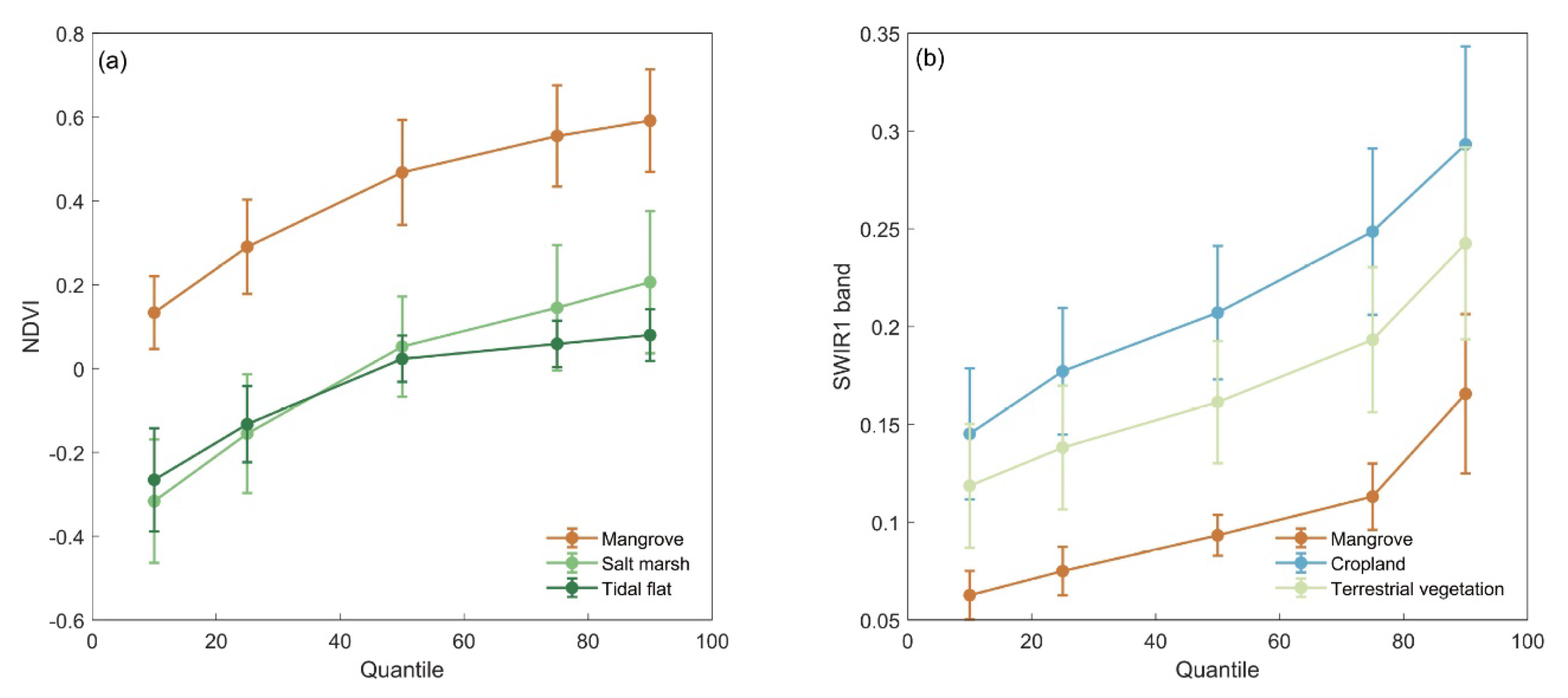
3.2. Spectral/Backscatter-Temporal Variability Features Extraction

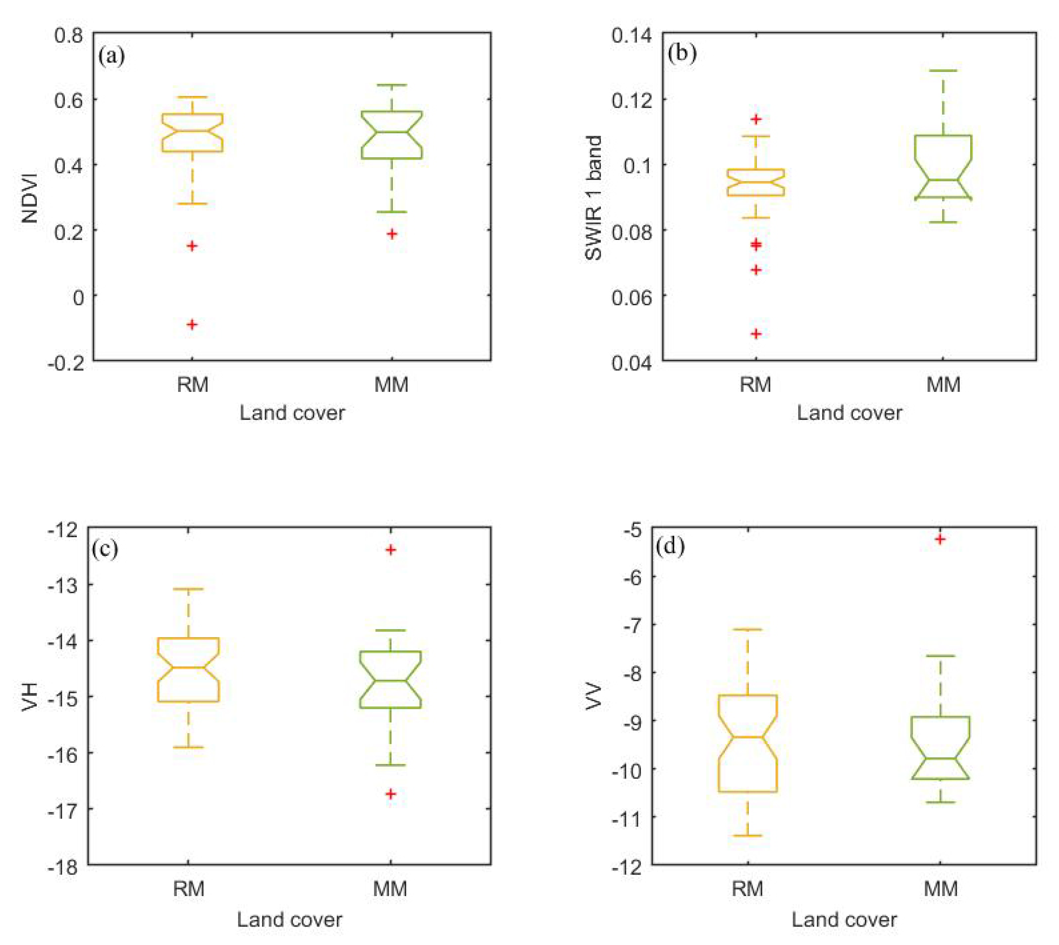
Previous studies have proven that the spectral/backscatter-temporal variability, generated by using remotely-sensed time-series data, could be used to effectively separate mangroves from other land cover types (e.g., salt marsh, tidal flats, cropland, and terrestrial vegetation) [27]. Here, we adopted five quantiles (10%, 25%, 50%, 75%, and 90%) of time-series imagery to quantitatively delineate the temporal profiles of spectral and backscatter signatures. The quantiles were calculated as follows: (1) combining all images during 2013 and 2018 into a multi-dimensional array; (2) for the pixels of each band, sorting all clear values from 2013 to 2018 and extracting quantiles requested. By employing the above five quantiles, it can be seen that mangroves show a remarkable difference from other land cover types. As shown in Figure 2, the quantile values of NDVI for mangroves are much higher than those for salt marsh and tidal flats, while the quantile values of the SWIR1 band for mangroves are much lower than those for cropland and terrestrial vegetation. Additionally, the Student’s t-test result also showed that the differences between the quantile values for mangroves and those for other land cover types are significant (significance level = 0.05).

The five metrics were generated for 10 spectral bands, 2 backscatter bands (VV, VH), 7 spectral indices bands (NDVI, NDWI, MNDWI, PSRI1, PSRI2, PSRI3) and 36 (3$\times \left(10+2\right)$) textural bands derived from 10 spectral bands, 2 backscatter bands, and 7 spectral indices. Finally, we in total identified 275 features per pixel.

3.3. Mapping Mangrove Forests with Random Forest

Random forest, a widely used machine learning algorithm, was applied to identify the mangrove forest, achieving a better accuracy of land cover map than any other algorithm [27,46]. This algorithm classifies the data by integrating votes from a mass of decision trees, which are built by fitting the features of training samples subsets generated randomly. There are three parameters governing the Random Forest algorithm: the number of trees (ntree), the minimum number of terminal seeds (nodesize), and the number of features (mtry) [47]. In our study, ntree was set to 200, since previous studies have found that if the number of decision trees is larger than 120, the accuracies of maps become more stable [27]. For the other two parameters, we adopted the default values (nodesize: 1; mtry: the square root of the number of all features). Finally, each classification result derived by using Random forest was recalculated using a $3\times 3$ spatial window [27].

To train the Random forest classifier, we collected 19378 training samples. The sample selection process contains two steps. (1) Picking sample sites. In our study, we manually selected sample sites (10 × 10 m, the size of Sentinel-2 pixel), which were evenly distributed and covered different land cover types (such as mangrove forest, water, cropland, terrestrial forest, or impervious surface) within the 10-km buffer zone along coastlines. (2) Interpreting samples as “mangrove forest” and “non-mangrove forest.” “Mangrove forest” was defined as areas in which the mangrove canopy cover is larger than 20%, while “non-mangrove forest” was defined as areas in which the area percentage of other land cover types (such as forests, shrubs, salt marshes, tidal flat, water, and cropland) is greater than 80%. For sample sites not distributed in the intertidal region, we interpreted them as “non-mangrove forest” because mangrove forests only grow in intertidal zone. For sample sites distributed in intertidal regions, we utilized Google Earth high-resolution imagery to determine whether an area was covered by mangrove forest, since, in Google Earth imagery, mangrove forests can be easily distinguished from other land cover types, such as salt marshes and tidal flat.

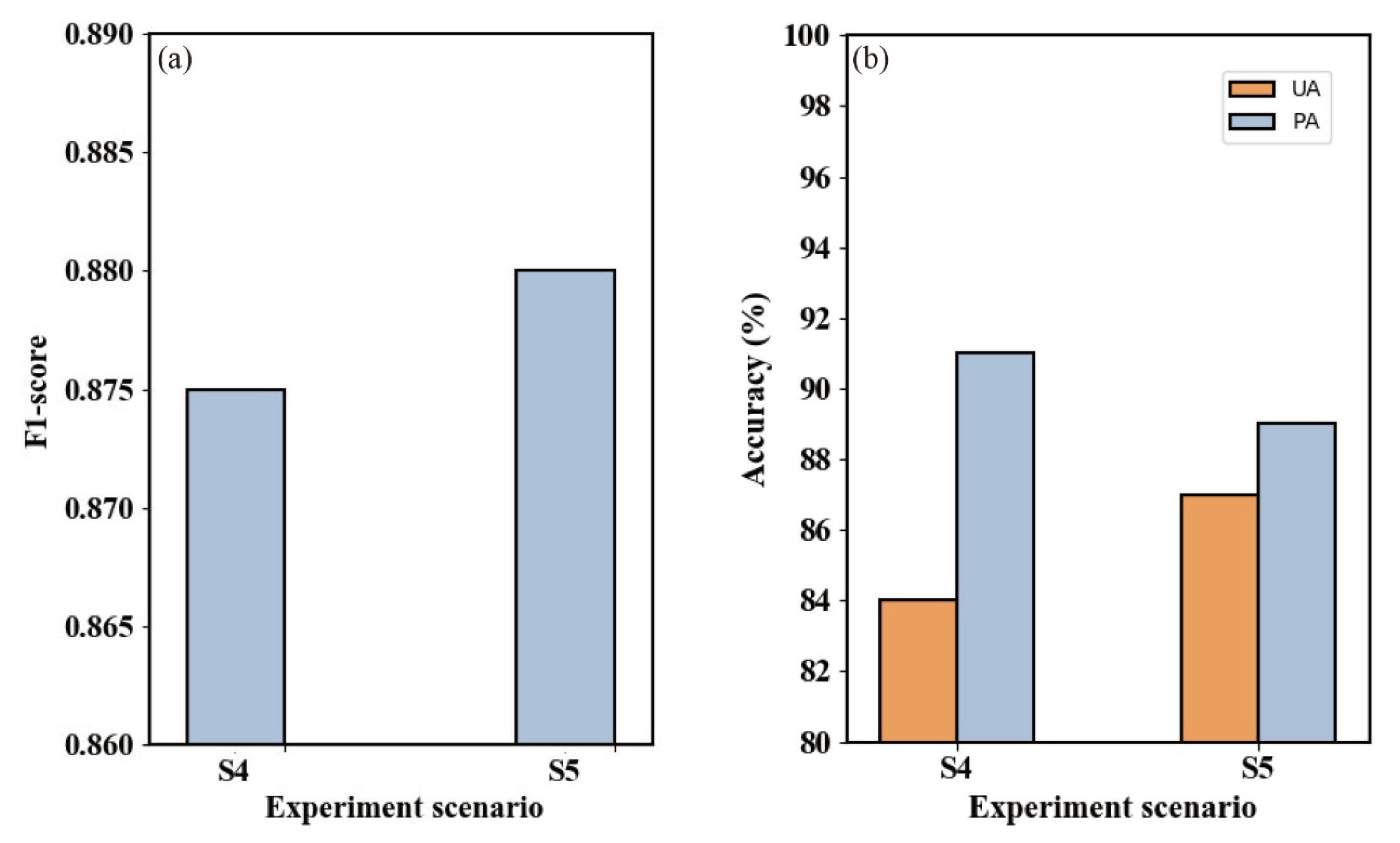
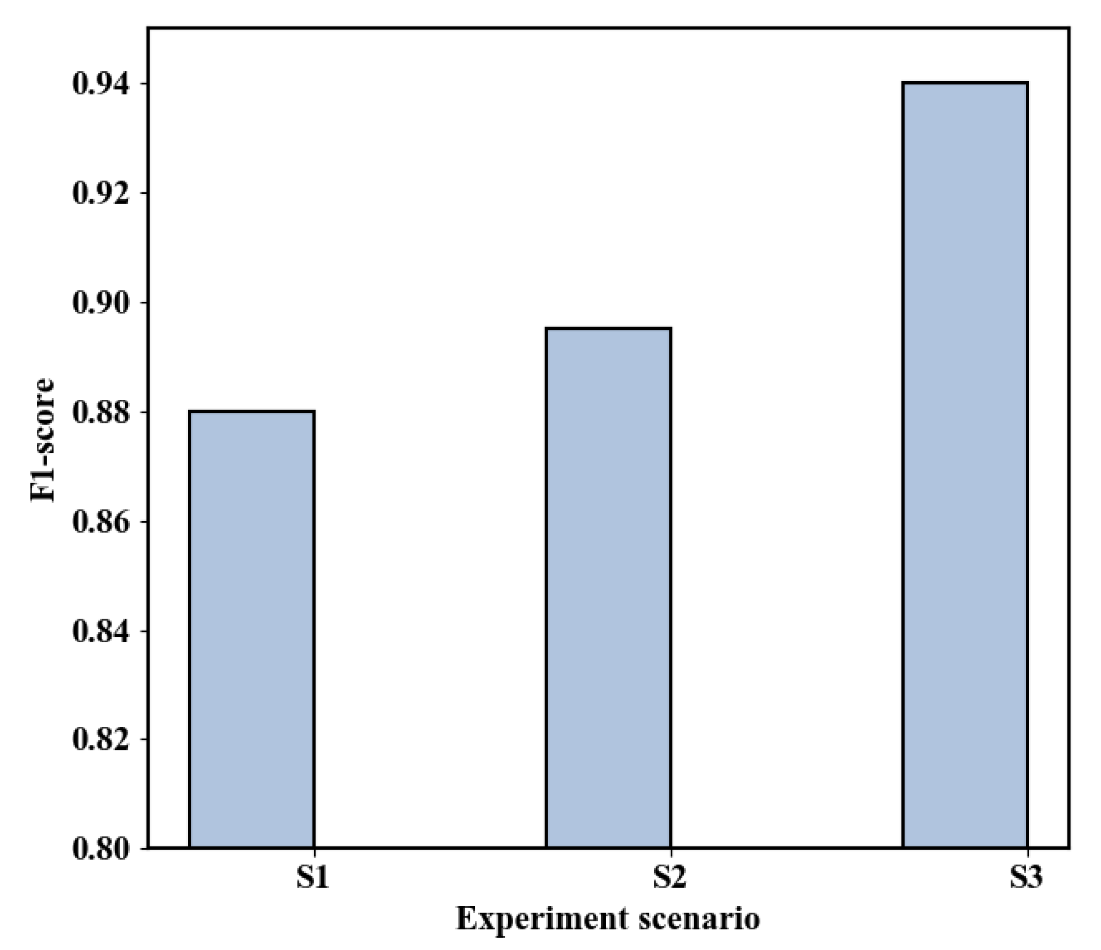
To explore an optimal combination of features from Sentinel-1 and Sentinel-2 time-series data for extracting mangroves, we conducted three experiments: (1) using Sentinel-1 data (S1 in

Table 4. Experiment designed in our study.

Scenario	Abbreviation	Input Features
1	S1	Backscatter-temporal features derived from Sentinel-1 SAR imagery (10%, 25%, 50%, 75%, and 90% quantiles of VV, VH; CON, ENT, and COR calculated from the above bands); Latitude and longitude; elevation, aspect, and slope derived from SRTM data
2	S2	Spectral-temporal features derived from Sentinel-2 MSI imagery (10%, 25%, 50%, 75%, and 90% quantiles of B2, B3, B4, B5, B6, B7, B8, B8A, B11, B12, NDVI, NDWI, MNDWI, PSRI1, PSRI2, PSRI3, and PSRI4; CON, ENT, and COR calculated from the above bands); Latitude and longitude; elevation, aspect, and slope derived from SRTM data
3	S3	Spectral/backscatter-temporal features derived from a combination of Sentinel-1 and Sentinel-2 data (10%, 25%, 50%, 75%, and 90% quantiles of B2, B3, B4, B5, B6, B7, B8, B8A, B11, B12, NDVI, NDWI, MNDWI, PSRI1, PSRI2, PSRI3, PSRI4, VV, and VH; CON, ENT, and COR calculated from all the above bands); Latitude and longitude; elevation, aspect, and slope derived from SRTM data

); (2) using Sentinel-2 data (S2 in Table 4); (3) using the combination of Sentinel-1 and Sentinel-2 data (S3 in Table 4).

3.4. Accuracy Estimation

The classification accuracy was quantitatively evaluated by applying validation samples. Based on a mangrove dataset integrating all results generated from all scenarios mentioned in Section 3.3, the locations of validation sample sites were determined by using a stratified random sampling. The interpretation method of these validation samples was the same as the method mentioned in Section 3.3. Finally, we got 1367 validation samples.

The above samples were applied to estimate producer’s accuracy, user’s accuracy, and F1-score of each mangrove forest map. The producer’s accuracy is the probability that a pixel was correctly classified as a given class [48]. The user’s accuracy is the probability that a pixel classified as a certain class in the map actually represents that class on the ground [48]. The F1-score is a useful index to assess class-level accuracy and is calculated from the harmonic mean between producer’s (PA) and user’s (UA) accuracy for mangroves as follows [49]:

$$\mathrm{F}1=\frac{2\times PA\times UA}{PA+UA}.$$

(4)

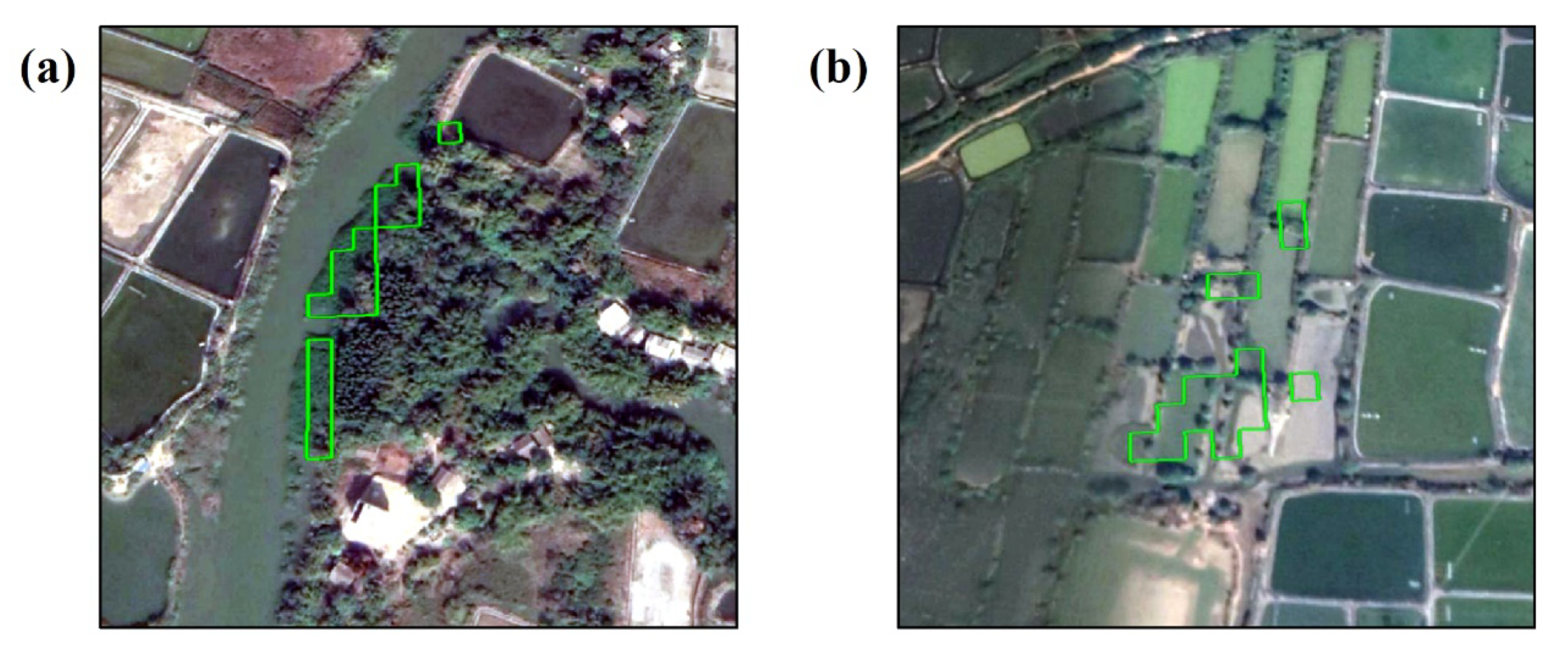
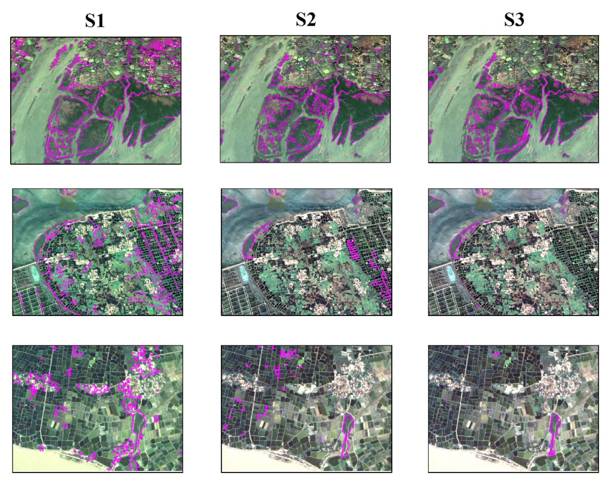
Additionally, we also qualitatively estimated the performance of our maps by overlaying them on high-resolution Google Earth imagery.

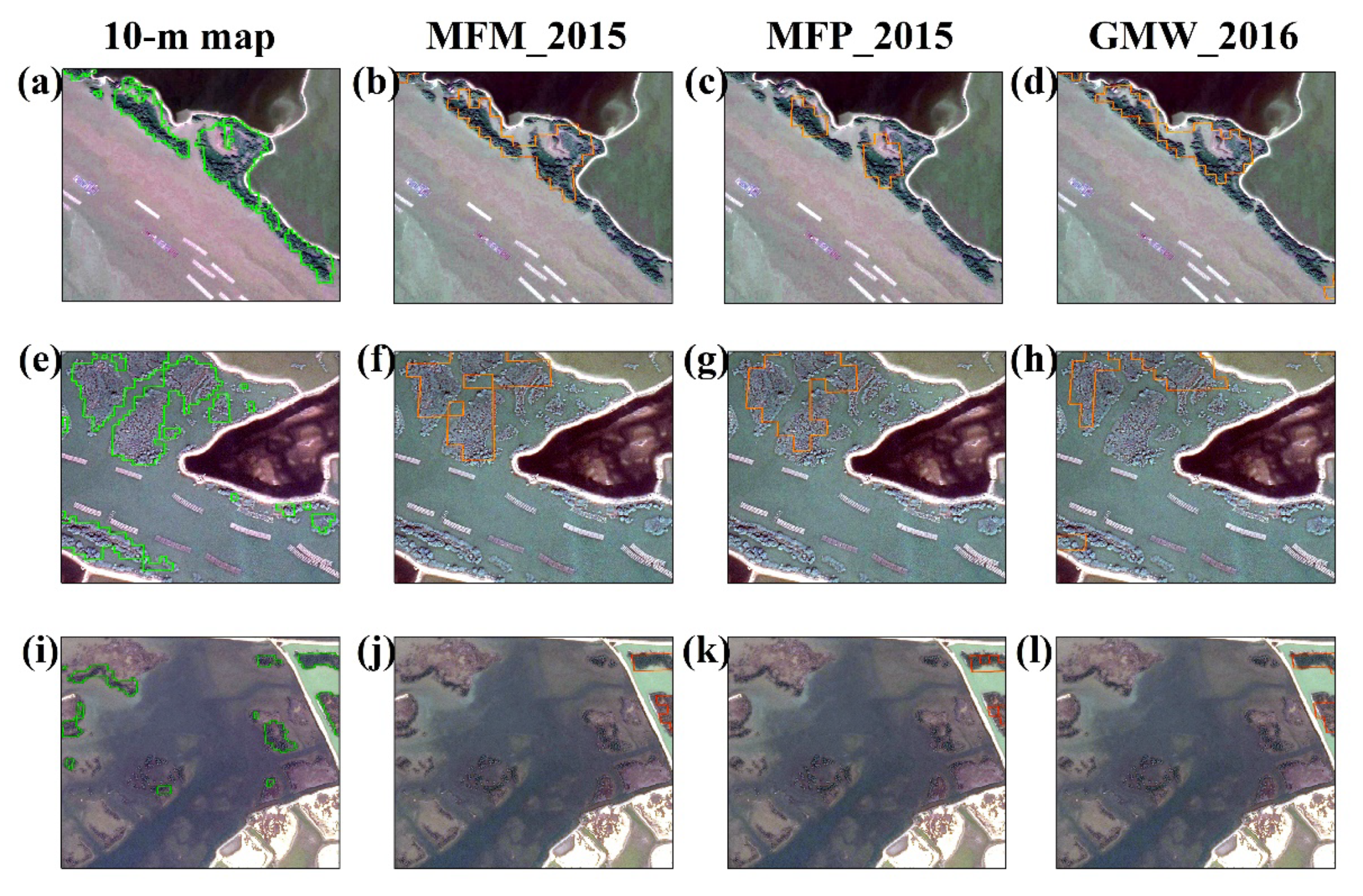
3.5. Comparison with Existing 30-m Mangrove Forests Products

Several regional and global mangrove products with 30-m spatial resolution have been generated from Landsat imagery. In this study, we mainly used three freely available products: (1) Mangrove forest map of China in 2015 by Chen et al. (2017) (MFM_2015) [22], which was mainly generated by using information of greenness, tidal inundation, and canopy coverage derived from time-series Landsat imagery. The map was downloaded from the website [50]. (2) Mangrove forest product of China in 2015 by Hu et al. (2018) (MFP_2015) [27], which was produced by adopting spectral-temporal variability metrics derived from time-series of Landsat imagery. This dataset was available from the website [51]. (3) Global mangrove watch in 2016 by Thomas et al. (2018) (GMW_2016) [23], which was derived from cloud-free Landsat mosaics and PALSAR data. 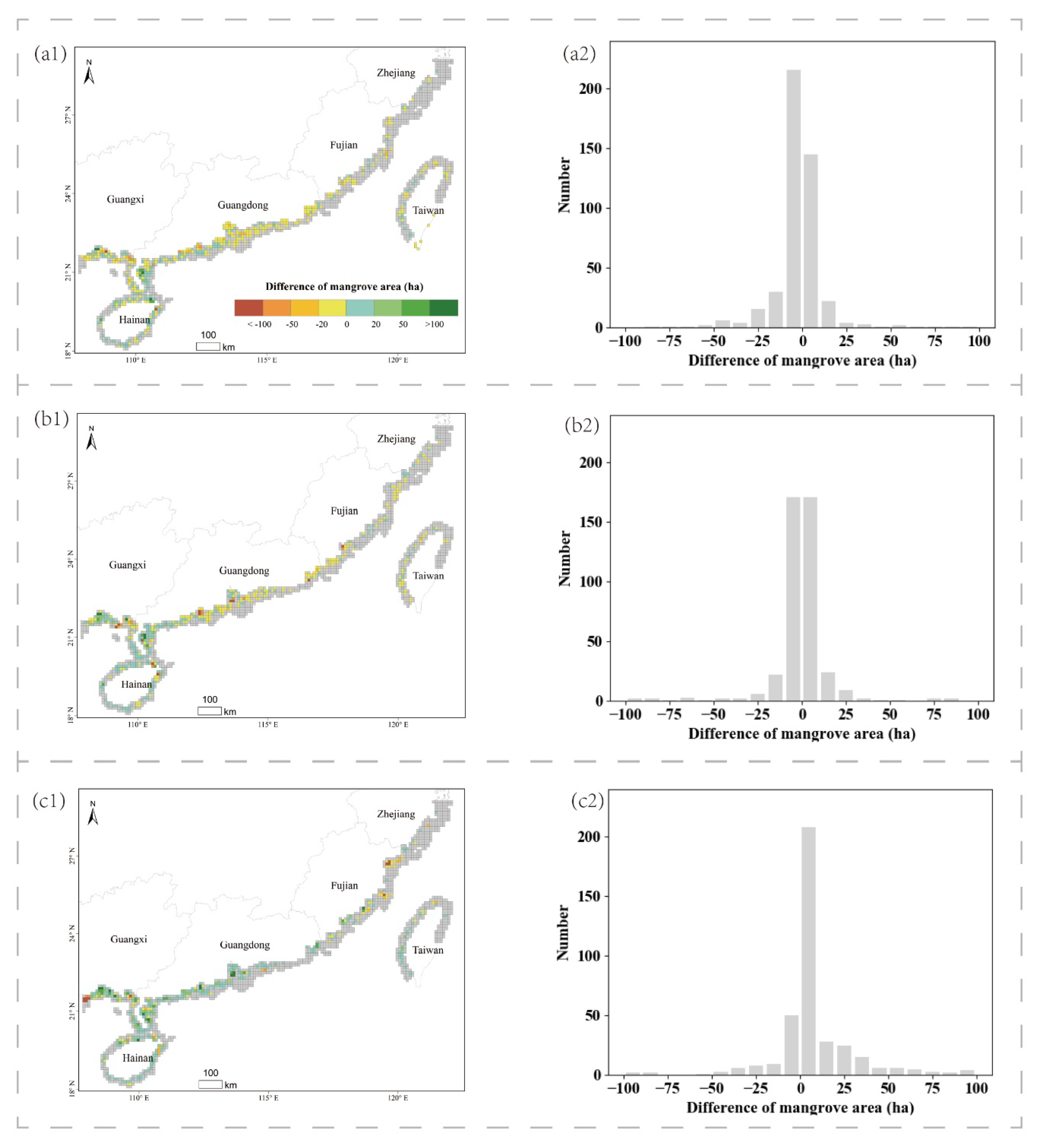We got this product from the website [52]. We aggregated all these maps to a common grid of 0.1° and calculated the area differences of mangrove forests between our 10-m map and the above 30-m products.

4. Results

4.1. Accuracy Assessment of Mangrove Forests Maps

Accuracy assessment of the mangrove forest maps derived from Sentinel-1 SAR imagery (S1), Sentinel-2 MSI imagery (S2), and a combination of Sentinel-1 and Sentinel-2 data (S3), was performed using 1367 validation samples, and the classification accuracy, including producer’s accuracy, user’s accuracy, and F1-score, were calculated. S1 and S2 yielded an F1-score of 0.88 and 0.895, respectively, while S3 had a higher F1-score (0.94) (Figure 3).

Table 5. The producer’s (PA) and user’s (UA) accuracy of Sentinel-1 (S1), Sentinel-2 (S2), and Sentinel-1/2 (S3) based mangrove maps.

	S1	S2	S3
PA (%)	87	90	94
UA (%)	89	89	94

shows the producer’s and user’s accuracy of S1, S2, and S3 used to generate the F1-score. Compared with S1 and S2, both the producer’s and user’s accuracies of S3 increased, indicating that combining Sentinel-1/2 data can effectively reduce mangrove map errors of commission (increased user’s accuracy) and omission (increased producer’s accuracy). Additionally, the producer’s accuracy of S1 was lower than that of S2 (Table 5), indicating that the Sentinel-2 derived map had a smaller overestimation of mangrove forests than Sentinel-1 derived maps.

Furthermore, based on Google Earth imagery, the performance of maps derived from S1, S2, and S3 was also evaluated. As shown in Figure 4, the S3 map showed an obvious improvement on mangrove extraction and error decrease, and the overestimation of the map derived from S1 was greater than that derived from S2, which is in accordance with the above accuracy assessment results.

4.2. Distribution of Mangroves in China in 2015 Derived from 10-m Map

4.2.1. Area and Spatial Distribution of Mangroves in China in 2015 Derived from 10-m Map

We applied the 10-m mangrove map derived by combining Sentinel-1/2 data to estimate the area and spatial distribution of mangroves in China circa 2015. In total, the mangrove forest area of China in 2015 was about 20003 ha. These mangroves are mainly distributed in the coastal zones of Guangxi (7000 ha), Guangdong (7786 ha), and Hainan (3927 ha) Province, which accounts for nearly 93.6% of the total mangrove area in China. The remaining mangroves in China are scattered in Hong Kong, Macao, Fujian, Zhejiang, and Taiwan. The spatial distribution of the above mangroves is shown in Figure 5 by aggregating mangrove areas to a common unit of 0.1°.

4.2.2. Area and Distribution of Small Mangrove Patches with Sizes Smaller than 1 Ha in China

Here, we defined the size of small mangrove patches, which are heterogeneous and disconnected with others, as being smaller than the minimum discriminating area (1 ha) of Landsat imagery. In general, the total area of small mangrove patches is 1741 ha, accounting for 8.7% of all the mangrove forests in China (Figure 6a), and the number (5646) of these small patches occupied a large percentage (74.5%) of total number of patches in China (Figure 6b). The spatial distribution of the above mangrove patches smaller than 1 ha is shown in Figure 7a by aggregating the number of these patches to a common unit of 0.1°. We found that Guangdong province, especially Zhanjiang region (Figure 7b), has a large number of small mangrove patches, and our 10-m map accurately identified them (Figure 7c,d).

Furthermore, we calculated the area of the small mangrove patches at the provincial level and their percentage in the total area of different provinces (

Table 6. The area of mangrove patches with size smaller than 1 ha in different regions.

	Area of Mangrove Patches (ha)	Percentage in Total Area of Small Mangrove Patches (%)	Percentage in the Whole Mangrove Area of Province (%)
Macao	0.7	0.04	8.8
Fujian	61.8	3.56	11.4
Guangdong	818.6	47	10.5
Guangxi	441.6	25.4	6.3
Hainan	344.3	19.8	8.8
Taiwan	47.4	2.7	16.7
Hong Kong	20.7	1.2	4.7
Zhejiang	6.0	0.3	46.9

). Similar to the above results (the number of small mangrove patches), Guangdong Province also occupies the largest area (819 ha) of small mangrove patches, and their percentage (47%) in the total area of small mangrove patches is nearly 50%. Additionally, we found that, in Fujian and Guangdong Provinces, the percentages of small mangrove patches in the total mangrove area are the highest (11.4%) and second (10.5%) highest, while the percentages in Hong Kong and Guangxi Province are the lowest (4.7%) and second (6.3%) lowest (Table 6). A large number of small patches in Guangdong and Fujian are likely to be caused by human disturbance, such as aquaculture and land reclamation [32].

4.3. Comparison of Sentinel-1/2 Derived Mangrove Forest Maps with Existing 30-m Products

We compared our 10-m map with existing 30-m products by calculating their differences of mangrove forest area at a grid of 0.1°. A positive value of area difference for a grid represents that the mangrove areas derived from our 10-m map are larger than those derived from 30-m products.

A substantial disagreement between the 10-m map and existing 30-m products was observed (Figure 8). For MFM_2015 (Figure 8a1,a2), the area difference values for 60.1% of the grids are negative. The number of grids whose area difference values are between −25 ha and 0 ha is the highest, and these grids are located over all the coastal zones with mangroves in China. Grids with positive area difference values, most of which are concentrated in the range of 0 ha and 25 ha, mainly occur in Guangxi, Hainan, and a few regions of Guangdong, such as the Zhanjiang region. For MFP_2015 (Figure 8b1,b2), the percentage of grids whose area difference values are larger than 0 ha (49.3%) is similar with those that are smaller than 0 ha (50.7%). The grids, whose area difference values are positive, are mainly distributed in the southwest coastal zones of China, including Guangxi, Hainan, and southwest of Guangdong, while these with negative values are located in the northeast coast of China, including Fujian, Zhejiang, Hong Kong, Macao, Taiwan, and northeast of Guangdong. For GMW_2016 (Figure 8c1,c2), the grids whose area difference values are larger than 0 ha are dominant (77.6%). The area difference values for most grids are between 0 ha and 25 ha and these grids occupy most regions with mangroves in China.

In addition, we also found that in the east coast of Zhanjiang, Guangdong Province, the area difference values for all the above 30-m products are larger than 100 ha. We compared the mangrove extraction results of the 10-m map with 30-m products (Figure 9). The comparison results show that in the Zhanjiang region, a lot of small mangrove patches (<1 ha) were not identified in any 30-m products, but were extracted in the 10-m map, indicating the necessity for generating a mangrove extent product with 10-m resolution. Furthermore, for all 30-m products, there also exists a few grids whose area difference values are smaller than −100 ha. The comparison results for subsets whose area difference values are smaller than −100 ha are shown in Figure 10. The 30-m products misclassified narrow rivers (Figure 10b,d) and salt marshes (Figure 10f) as mangroves, but the 10-m map accurately delineated the mangrove extent (Figure 10a,c,e).

5. Discussion

5.1. Whether Four Red Edge Bands in Sentinel-2 Data Improves the Capability of Msi Imagery on Extracting Mangrove Forest

Red edge bands are sensitive to the biophysical features (e.g., leaf chlorophyll and water content) of vegetation [53]. To explore the effect of four red edge bands in Sentinel-2 MSI on extracting the mangrove forest, we conducted two experiments: Scenario 4 (S4) and Scenario 5 (S5), and estimated their classification accuracies. The mangrove extraction result of S4 was derived by excluding four red edge bands, while that of S5 was generated by adding four red edge bands. Specifically, the input features of S4 and S5 are: (1) 10%, 25%, 50%, 75%, and 90% quantiles of B2, B3, B4, B8, B11, B12, NDVI, NDWI, MNDWI; Latitude, longitude, elevation, aspect, and slope; (2) 10%, 25%, 50%, 75%, and 90% quantiles of B2, B3, B4, B5, B6, B7, B8, B8A, B11, B12, NDVI, NDWI, MNDWI, PSRI1, PSRI2, PSRI3, PSRI4; Latitude, longitude, elevation, aspect, and slope.

The classification accuracy estimation results are shown in Figure 11. For S4 and S5, the F1-scores, reflecting the class-level accuracy, are nearly the same (0.875 VS. 0.88), and the producer’s accuracy (UA) and user’s accuracy (PA), which separately represent the omission errors and commission errors of mangrove maps, are also similar (UA: 84% vs. 87%; PA: 91% vs. 89%). This indicates that the four red edge bands make little contribution to mangrove extraction.

5.2. Error Sources of 10-m Mangrove Map

Based on high-resolution Google Earth imagery, we explored the error sources of 10-m mangrove maps derived from a combination of Sentinel-1 SAR and Sentinel-2 MSI imagery. We found that pixels, which were a mixture of evergreen vegetation and yearlong water bodies (especially at the edge of rivers and aquaculture ponds), were the main error source (Figure 12) due to the similarity of spectral/backscatter variability between mangroves and misclassified pixels. As an example, in Figure 13, for mangroves and misclassified pixels, the median variation ranges of both spectral (such as NDVI and SWIR 1 in Figure 13a,b) and backscatter (VV and VH in Figure 13c,d) bands overlap, revealing that features used in this study cannot effectively separate mixing evergreen vegetation with water from mangroves. This source of error was also mentioned in 30-m mangrove maps derived from Landsat imagery [22,27]. Therefore, in the future, we should explore effective identification features to reduce the above errors.

5.3. Implications for Mangrove Ecosystems and Future Research

The 10-m mangrove map at a national scale generated from Sentinel imagery provides more detailed information than previous 30-m products about the spatial distribution and extent of mangroves, especially mangroves with small size. This information is valuable for research on estimating mangrove ecosystem functions and services. Firstly, the advanced mangrove map with 10-m resolution can contribute to the improvement of carbon storage estimation. Previous studies have shown that the spatial distribution and area of mangroves are the baseline for estimating carbon storage of mangroves at large scales, and the deficiency of the high-resolution mangrove forest map is one of the main reasons for the large uncertainty in carbon storage estimation [14,54]. Secondly, the 10-m map, which can identify small mangrove patches, is helpful to study the role of mangrove habitat connectivity in ecosystem services. Previous research has demonstrated that small mangrove patches can interconnect adjacent coastal marine ecosystems (such as salt marshes, and coral reefs), and allow for easier movement and dispersal for coastal species, contributing to the establishment and growth of ecosystems [55,56]. Thirdly, this 10-m map is also conducive in assessing the effectiveness of protection and restoration strategies on mangrove ecosystems [57]. Since 2000, Chinese government institutions have taken initiatives to plant and rehabilitate mangroves. These planted and regenerated mangroves with small size are difficult to observe in 30-m maps, but can be extracted in 10-m maps.

In addition, the approach (combining Sentinel-1/2 data) adopted in this study has been proven to be useful in detecting mangrove forests along the whole coastal zones of China, which are characterized by heterogeneity and complexity [27,32]. Therefore, it has potential to be transferable globally in the future.

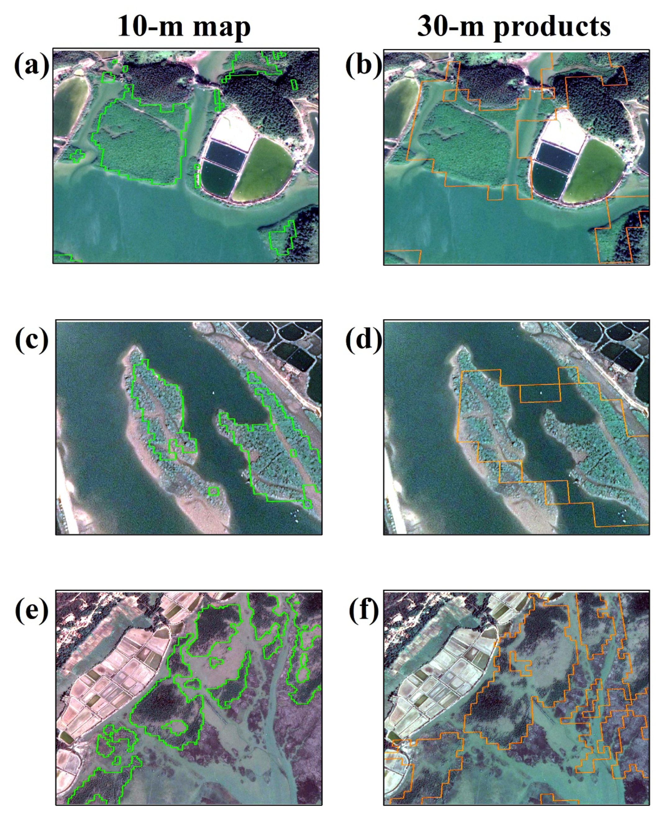
6. Conclusions

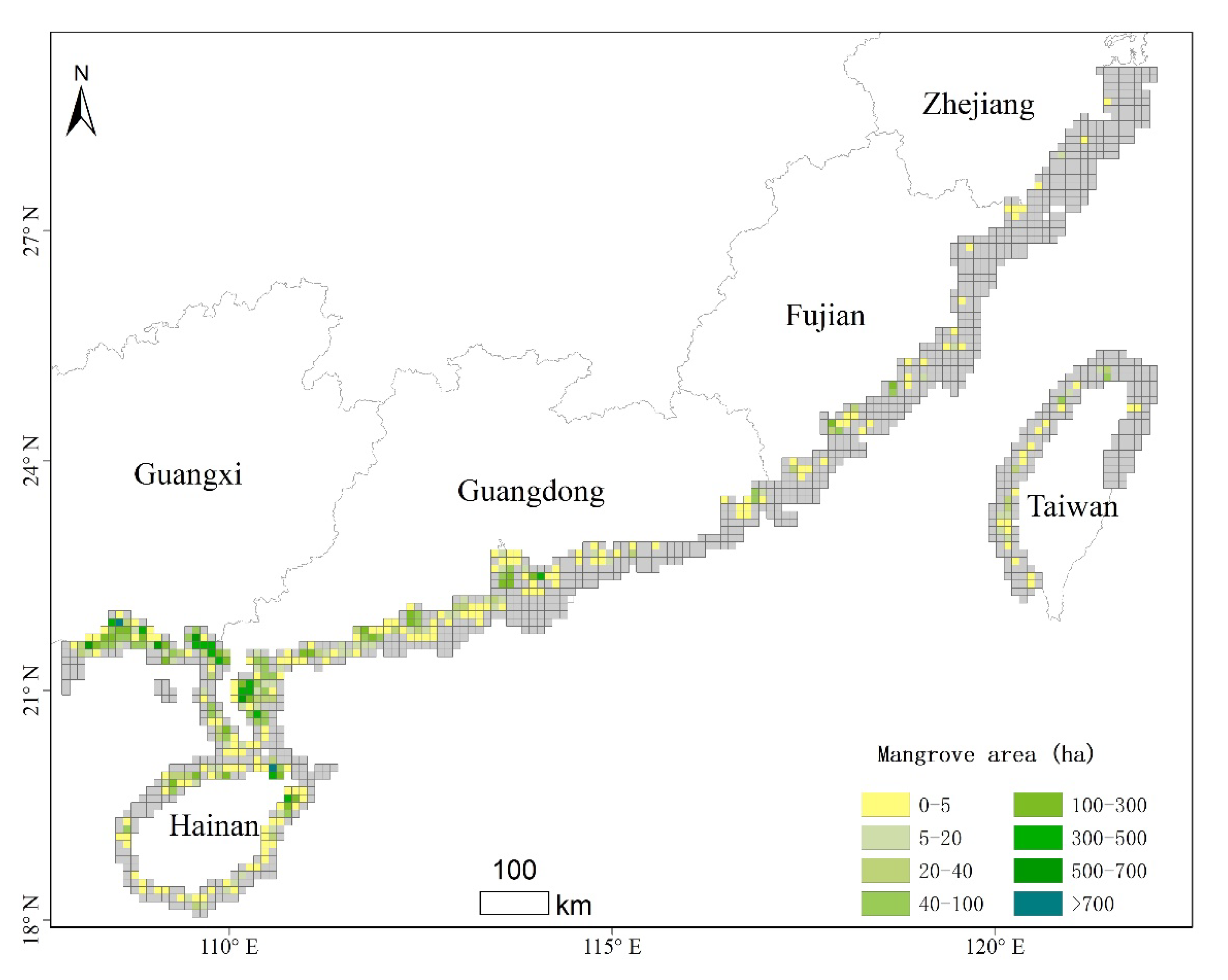
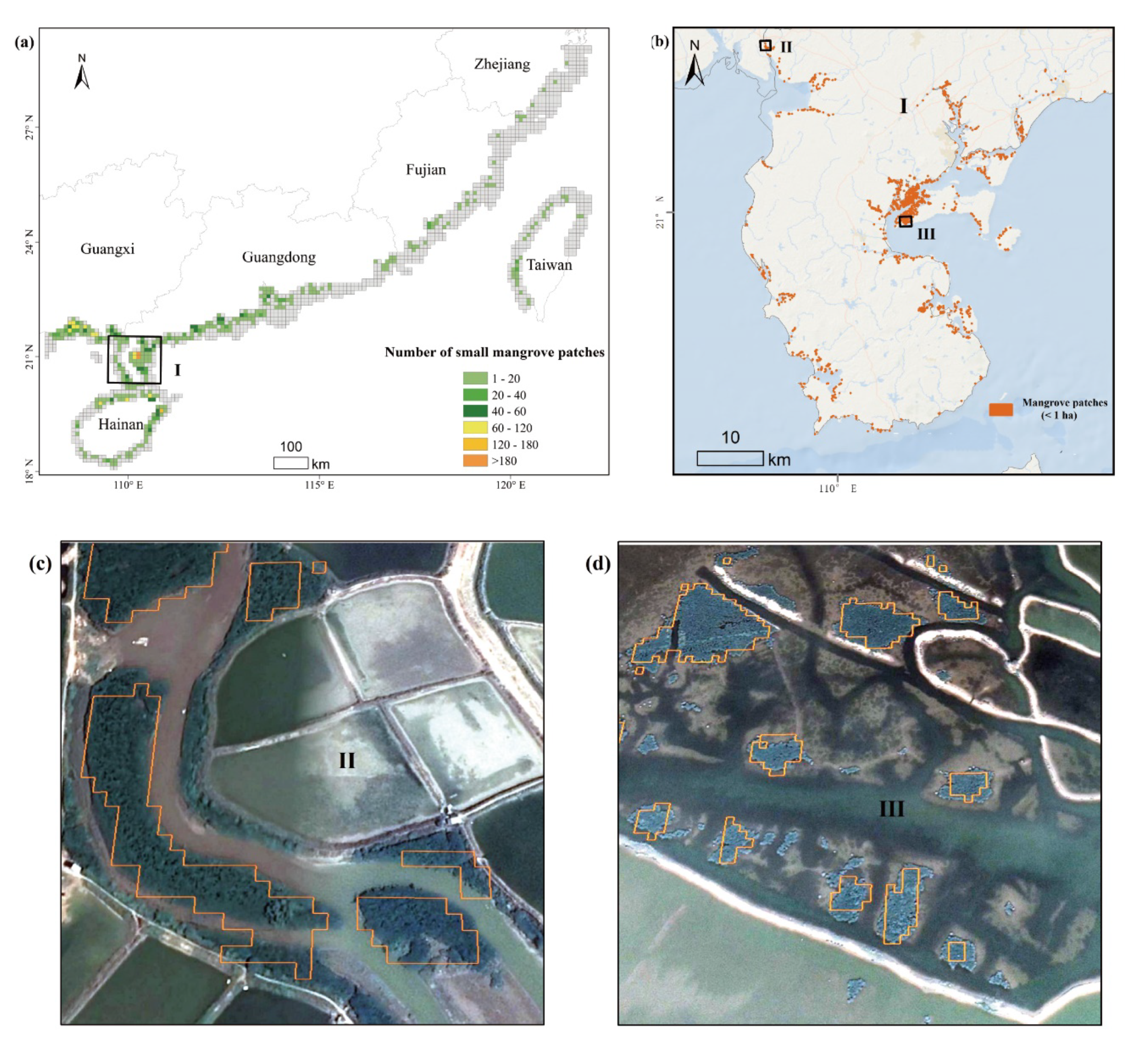
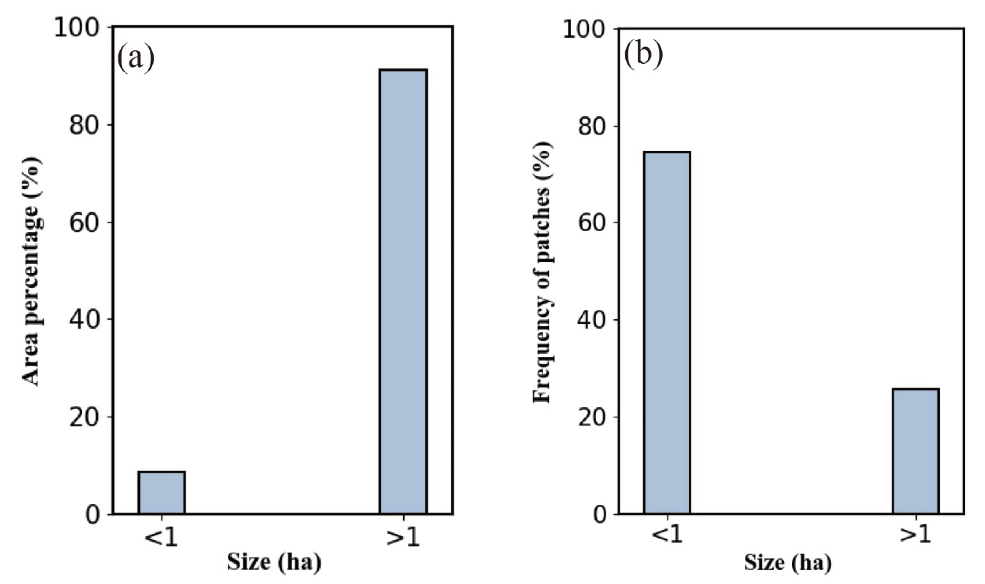
This study advances mangrove forest mapping in China by using time-series Sentinel-1 C-band SAR and Sentinel-2 MSI imagery based on GEE, and demonstrates that Sentinel imagery with 10-m resolution has the capability of accurately detecting national-scale mangrove forests. Small mangrove patches (<1 ha), which are difficult to extract using Landsat imagery with 30-m resolution, can be easily identified in the 10-m mangrove map. When applying Sentinel imagery to mapping national-scale mangroves, we found that the combination of Sentinel-1/2 time-series data is the optimal approach. In addition, we also found that the four red edge bands in Sentinel-2 make little contribution to mangrove extraction. Generally, the 10-m mangrove map, derived by combining Sentinel-1 and Sentinel-2 data, identified a total of 20,003 ha of mangrove forest in China. Among these, the total area of small mangrove patches (<1 ha) was 1741 ha, occupying 8.7% of the whole area of mangroves in China. At the provincial level, Guangxi, Guangdong, and Hainan account for nearly 93.6% of the total mangrove area in China. The largest area (819 ha) of small mangrove patches is located in Guangdong Province, and in Fujian, the percentage of small mangrove patches in the total mangrove area is the highest (11.4%). The above 10-m mangrove dataset in China can be used to analyze landscape fragmentation, quantify the budget of coastal carbon, and take effective steps to protect mangroves and restore degradation. In addition, the approach developed in our study could feasibly be used to map 10-m mangrove forests at continental and global scales based on the GEE.