Introducing an Improved GRACE Global Point-Mass Solution—A Case Study in Antarctica

Abstract

In the so-called point-mass modeling, surface densities are represented by point masses, providing only an approximated solution of the surface integral for the gravitational potential. Here, we propose a refinement for the point-mass modeling based on Taylor series expansion in which the zeroth-order approximation is equivalent to the point-mass solution. Simulations show that adding higher-order terms neglected in the point-mass modeling reduces the error of inverted mass changes of up to 90% on global and Antarctica scales. The method provides an alternative to the processing of the Level-2 data from the Gravity Recovery and Climate Experiment (GRACE) mission. While the evaluation of the surface densities based on improved point-mass modeling using ITSG-Grace2018 Level-2 data as observations reveals noise level of approximately 5.77 mm, this figure is 5.02, 6.05, and 5.81 mm for Center for Space Research (CSR), Goddard Space Flight Center (GSFC), and Jet Propulsion Laboratory (JPL) mascon solutions, respectively. Statistical tests demonstrate that the four solutions are not significant different (95% confidence) over Antarctica Ice Sheet (AIS), despite the slight differences seen in the noises. Therefore, the estimated noise level for the four solutions indicates the quality of GRACE mass changes over AIS. Overall, AIS shows a mass loss of −7.58 mm/year during 2003–2015 based on the improved point-mass solution, which agrees with the values derived from mascon solutions.

1. Introduction

The observations acquired by the time-resolved satellite gravimetry namely Gravity Recovery and Climate Experiment (GRACE) have provided essential information on the global mass changes since April 2002 [1]. For instance, the monthly fields of mass changes inverted from GRACE observations have been used in monitoring ice sheet and glacier mass balance as well as for understanding their contributions to sea level changes (e.g., Reference [2]). GRACE monthly solutions of the time-varying Earth’s gravity field are usually expressed in terms of spherical harmonic coefficients called Level-2 data. The Level-2 products are freely distributed by the centers identified in the GRACE Science Data System (SDS). These centers are the University of Texas Center for Space Research (CSR, [3]), the NASA Jet Propulsion Laboratory (JPL, [4]), and the German Research Centre for Geosciences (GFZ, [5]). Likewise, other institutions have provided independent solutions for Level-2 data based on alternative approaches (see, e.g., References [6,7,8,9,10,11,12]). Moreover, the recently established International Combination Service for Time-variable Gravity Fields (COST-G) generates combined monthly Level-2 data using the individual solutions of different analysis centers (cf. References [13,14]). However, the GRACE Level-2 data suffer from poor observability of east-west gradients [15] manifested as “stripes” in the derived maps of mass changes [16]. These stripes are conventionally removed using isotropic (degree-dependent) and anisotropic (degree- and order-dependent) filters associated with an anisotropic decorrelation procedure (see, e.g., References [16,17,18]).

As an alternative to the spherical harmonic representation of surface densities, the use of mass concentration (mascon) solutions allows for convenient applications of a priori information to reduce the striping since the basis functions are represented locally rather than globally. Mascon solutions use GRACE observations (e.g., K-band range-rate, KBR) accumulated over the entire month to invert for a global solution (e.g., Reference [19]), in which the surface densities of single layers are the unknown parameters for the gravity field. Many mascon approaches using GRACE KBR data have been presented (see, e.g., References [15,20,21,22,23,24,25]), at which analysis centers such as CSR [25], JPL [15], and the Goddard Space Flight Center (GSFC, [20]) provide solutions to the public. Unconstrained mascon and unfiltered spherical harmonic solutions are somewhat similar since their respective signal variances show almost the same power at different frequencies (cf. Reference [26,27]). Consequently, the choice of one or another solution generally will depend on the users’ experience and needs. The constrained mascon solutions, forwarded as Level-3 data (e.g., gridded mass changes), might be the best choice for most users since Level-2 data (i.e., spherical harmonic coefficients) require a handful of post-processing procedures (see, e.g., References [16,28,29]).

The mascon representation of surface densities can also be fitted to the GRACE Level-2 rather than to the original GRACE Level-1b data (see, e.g., References [30,31,32]). This procedure represents a post-processing method for the Level 2 data [15] in which the anisotropic de-correlation (e.g., Reference [16]) can be omitted to improve the sampling characteristics of the recovered surface masses (see Reference [31] for details). Furthermore, the synthesized residual gravitational attraction, projected at GRACE’s altitude, can also be used as a form of Level-2 processing/post-processing by applying inverse modeling parametrized by surface densities of single layer (e.g., Reference [33]) or point-mass modeling (e.g., Reference [34]). Inverse point-mass modeling as a post-processing of GRACE Level-2 data has been used to estimate ice mass changes in Greenland [34,35,36,37] and Antarctica [37,38], as well as to reveal groundwater storage changes in Yangtze River basin [39]. However, as the gravitational potential (or its radial derivative that provides the gravitational attraction) is defined by Newton’s integral, which is an elliptic integral of the first kind when expressed in terms of geocentric coordinates, point-mass modeling is just an approximate solution.

Therefore, the question of whether the deviations of the point-mass solution from the original Newton’s integral are negligible needs to be addressed, which has not been considered in previous works [34,35,36,37,38,39]. To investigate this is important because the inverse point-mass modeling approach has been shown as a feasible method for post-processing GRACE Level-2 data as concluded by Baur & Sneeuw [36], and it has been used to estimate Antarctica ice mass changes and associated contribution to sea-level rise (cf. Reference [38]), which is a global concern. To this end, the objectives of this study are tripartite: (i) to investigate the inverse modeling using point-mass solution; (ii) to present an improved solution for the point-mass representation, and (iii) to estimate mass changes of Antarctica using the improved point-mass method. The approach to improve the point-mass modeling is based on Taylor series expansions of the kernel function of Newton’s integral related to the gravitational effects of so-called tesseroids [40]. Tesseroids are elementary bodies resulting from the subdivision of the sphere (or ellipsoid) into elements bounded by geographical grid lines and surfaces of constant height. The procedure proposed in this paper is a reduction of the 3-D spherical tesseroid approach [40] to the 2-D case. Noteworthy, the use of original formulae referring to 3-D bodies would add inconveniences because the inverse modeling would contain nonlinear terms.

The subsequent sections of the study are structured as follows: Section 2 presents a description of the datasets and methods. The results are presented in Section 3 followed by their discussions in Section 4. The conclusions of the study are provided in Section 5.

2. Material and Methods

2.1. Methodology

2.1.1. The Improved Point-Mass (IPM) Solution

Considering that the static gravity field of the Earth has been removed, the time variable residual gravitational potential as sensed by the satellite gravimetry can be seen as a column from the satellite’s altitude to the center of the Earth due to large-scale mass variations. If hydrological mass variations are in the focus of interest, the other contributions from atmosphere and ocean mass variations, polar motion, solid and oceanic tides, and solid Earth variations (e.g., due to glacial isostatic adjustment—GIA—and mass loadings), can be reduced using background models and assumptions of a deformable Earth, respectively. Thus, Newton’s integral for the residual gravitational potential ($\delta V$) due to surface densities, which are assumed to be concentrated on a virtual layer of water thickness $\mathsf{\Delta }r$ (equivalent water height—hereafter abbreviated as e.w.h.) on Earth’s surface, is given as:

$$\begin{array}{cc}\hfill \delta V(r,\phi ,\lambda )=& \frac{1}{2}G{\varrho }_{\mathrm{w}}\sum _k\left\{\underset{{\lambda }_1}{\overset{{\lambda }_2}{\int }}\underset{{\phi }_1}{\overset{{\phi }_2}{\int }}\right[\ell (r^{\prime }+3rcos\psi )+r^2(3{cos}^2\psi -1)\hfill \\ \hfill & \times ln(\ell +r^{\prime }-rcos\psi ){]}_{r^{\prime }=R}^{r^{\prime }=R+\mathsf{\Delta }r}cos{\phi }^{\prime }{\phi }^{\prime }{\lambda }^{\prime }{\}}_k,\hfill \end{array}$$

(1)

which was discretized for each panel k. In Equation (1), G is the Newtonian constant of gravitation ($G=6.67408\times {10}^{-11}$ m${}^3$kg${}^{-1}$s${}^{-2}$, cf. Reference [41]), ${\varrho }_{\mathrm{w}}$ is the density of fresh water (position-dependent, which can be considered constant $\sim 1000$ kg/m${}^3$). The Euclidean distance (ℓ) between the (attracted) computation point $P(r,\phi ,\lambda )$ and the running integration (attracting) point $Q(r^{\prime },{\phi }^{\prime },{\lambda }^{\prime })$ is given by the al-Kāshi theorem:

$$\ell =\sqrt{r^2+{r^{\prime }}^2-2r{r}^{\prime }cos\psi },$$

(2)

with $\psi$ being the spherical distance as:

$$cos\psi =sin\phi sin{\phi }^{\prime }+cos\phi cos{\phi }^{\prime }cos(\lambda -{\lambda }^{\prime }).$$

(3)

Furthermore, $\mathsf{\Delta }r=r_2-r_1$ is the e.w.h. in meters, which is assumed to generate the residual gravitational potential $\delta V$ at the satellite gravimetry.

The integral in Equation (1) is an elliptic integral in terms of the geocentric spherical coordinates (${\phi }^{\prime },{\lambda }^{\prime }$) and, as such, it is not integrable in elementary terms. Taking the first-order approximation of the kernel in Equation (1) into account, that is, neglecting $\mathcal{O}\left(\mathsf{\Delta }{r}^2\right)$, which gives $2\mathsf{\Delta }r{R}^2/{\ell }^{″}$ (see Equation (A10) in Appendix A), the resulting integral

$$\begin{array}{c}\hfill \delta V(r,\phi ,\lambda )=G{\varrho }_{\mathrm{w}}\sum _k\mathsf{\Delta }{r}_k\{\underset{{\lambda }_1}{\overset{{\lambda }_2}{\int }}\underset{{\phi }_1}{\overset{{\phi }_2}{\int }}\frac{R^{2}cos{\phi }^{\prime }}{{\ell }^{″}}\mathsf{d}{\phi }^{\prime }\mathsf{d}{\lambda }^{\prime }+\mathcal{O}\left(\mathsf{\Delta }{r}^2\right){\}}_k,\end{array}$$

(4)

becomes an elliptic integral of the first kind. In Equation (4), ${\ell }^{″}$ is the Euclidean distance given by (A9), and the Landau symbol $\mathcal{O}\left(\mathsf{\Delta }{r}^2\right)$ indicates that the second-order terms in $\mathsf{\Delta }r$ are omitted. Given the first-order approximation of the kernel appearing in the surface integral in Equation (4), and considering the surface density $\mu$ given by ${\varrho }_{\mathrm{w}}·\mathsf{\Delta }r$, the remain integral becomes equivalent to the potential of a single layer (or density layer, simple layer). The so-called mascon solutions represent the time-varying gravity field as the potential of a single layer [21]. Such solutions assume that the mass changes take place at the Earth’s surface [42]. This assumption is somewhat valid since the time-varying signals mainly reflect the superficial processes such as the water cycle given that the non-surficial sources such as GIA have been removed. Consequently, the challenges due to the non-uniqueness of the inversion of the volume integral to find a unique distribution of masses enclosed by a body given the external potential as observations are overcome when considering the surface integral for the Earth’s surface, of which the inversion is unique [42].

Since elliptic integrals occur in Equation (4), it cannot be solved by elementary integration. Therefore, it is proposed to perform a Taylor series expansion of the integrand in Equation (4), that is, the kernel function, and its subsequent integration. Noteworthy, this has already been suggested for the volume integral by, for example, Heck & Seitz [40], Wild-Pfeiffer [43], and Grombein et al. [44]. The solution presented by these authors has been proposed in the context of the forward modeling of the gravity field due to the topographic masses, and it would become a nonlinear problem in the present context. Nevertheless, the kernel of the integral given in Equation (4) (that is, second-order and higher terms in $\mathsf{\Delta }r$ were not considered) can be formulated in Taylor series as:

$$\begin{array}{cc}\hfill K(R,{\phi }^{\prime },{\lambda }^{\prime })& =\frac{R^{2}cos{\phi }^{\prime }}{{\ell }^{″}}\hfill \\ \hfill & =\sum _{i,j=0}^{\infty }{K}_{i,j}\frac{{({\phi }^{\prime }-{\phi }_0)}^i}{i!}\frac{{({\lambda }^{\prime }-{\lambda }_0)}^j}{j!},\hfill \end{array}$$

(5)

where the coefficients $K_{i,j}$ are the partial derivatives of the integral kernel K defined by

$$K_{i,j}:={\left.\frac{{\partial }^{i+j}}{\partial {{\phi }^{\prime }}^i\partial {{\lambda }^{\prime }}^j}K(R,{\phi }^{\prime },{\lambda }^{\prime })\right|}_{({\phi }^{\prime },{\lambda }^{\prime })=({\phi }_0,{\lambda }_0)}.$$

(6)

The coefficients $K_{i,j}$ in Equation (6) depend on the relative positions of the computation point $P(r,\phi ,\lambda )$ at satellite altitude and the geometric center $Q_0(R,{\phi }_0,{\lambda }_0)$ of the spherical panel (i.e., the Taylor point defined by ${\phi }_0=({\phi }_1+{\phi }_2)/2$ and ${\lambda }_0=({\lambda }_1+{\lambda }_2)/2$). In this case, the zeroth-order coefficient $K_{0,0}$ results in

$$K_{0,0}=\frac{R^{2}cos{\phi }_0}{{{\ell }^{″}}_0},$$

(7)

where ${{\ell }^{″}}_0$ is given by Equation (A9) at which $\psi ={\psi }_0$ (center of the panel). The second-order coefficients $K_{2,0}$ and $K_{0,2}$, computed by means of Equation (6), are given as

$$\begin{array}{cc}\hfill K_{2,0}=& \frac{R^2}{{{\ell }^{″}}_0^5}\{-cos{\phi }_0(r^2+R^2)\left[r^2+R^2-rRsin\phi sin{\phi }_0\right]\hfill \\ \hfill & +r^2{R}^{2}cos{\phi }_0\left[{sin}^2\phi (3-{sin}^2{\phi }_0)-{cos}^2\phi (2-{sin}^2{\phi }_0){cos}^2(\lambda -{\lambda }_0)\right]\hfill \\ \hfill & +rRcos\phi (3-{sin}^2{\phi }_0)\left[r^2+R^2-2Rsin\phi sin{\phi }_0\right]cos(\lambda -{\lambda }_0)\},\hfill \end{array}$$

(8)

and

$$\begin{array}{cc}\hfill K_{0,2}=& -\frac{r{R}^{3}cos\phi {cos}^2{\phi }_0}{{{\ell }^{″}}_0^5}\left[{{\ell }^{″}}_0^{2}cos(\lambda -{\lambda }_0)-3rRcos\phi cos{\phi }_0{sin}^2(\lambda -{\lambda }_0)\right],\hfill \end{array}$$

(9)

respectively. Note that in the context presented here, where $R<r$, no singularities can occur in Equations (7)–(9) when $\psi =0^{\circ }$.

Considering a Taylor series expansion up to degree 3, the gravitational potential according to the discretization presented in Equation (4) can be expressed by

$$\begin{array}{cc}\hfill \delta V(r,\phi ,\lambda )=& G{\varrho }_{\mathrm{w}}\mathsf{\Delta }\phi \mathsf{\Delta }\lambda \sum _k{\mathsf{\Delta }r}_k{\left[K_{0,0}+\frac{1}{24}(K_{2,0}\mathsf{\Delta }{\phi }^2+K_{0,2}\mathsf{\Delta }{\lambda }^2)+\mathcal{O}\left({\mathsf{\Delta }}^4\right)\right]}_k,\hfill \end{array}$$

(10)

where $\mathsf{\Delta }\phi ={\phi }_2-{\phi }_1$ and $\mathsf{\Delta }\lambda ={\lambda }_2-{\lambda }_1$ denote the horizontal dimensions of a spherical panel k. In Equation (10), $\mathcal{O}\left({\mathsf{\Delta }}^4\right)$ indicates that the fourth-order terms in $\mathsf{\Delta }\phi$ and $\mathsf{\Delta }\lambda$ are omitted. That is, Equation (10) is approximate (accurate) up to third-order terms. Due to the specific choice of the Taylor point $Q_0$, only the terms with even powers of i and j in the series expansion remain after integration. In the case of ${\phi }^{\prime }$, the same holds for ${\lambda }^{\prime }$, the remaining even power can be verified by inserting Equation (5) into Equation (4), which provides:

$$\begin{array}{cc}\hfill \underset{{\phi }_1}{\overset{{\phi }_2}{\int }}{K}_{i,0}\frac{{({\phi }^{\prime }-{\phi }_0)}^i}{i!}\mathsf{d}{\phi }^{\prime }& =\underset{-{}^{\mathsf{\Delta }\phi }/{}_2}{\overset{+{}^{\mathsf{\Delta }\phi }/{}_2}{\int }}{K}_{i,0}\frac{{\left({\phi }^{*}\right)}^i}{i!}{\phi }^{*}\hfill \\ \hfill & =K_{i,0}\frac{\mathsf{\Delta }\phi \left[{\left(\mathsf{\Delta }\phi \right)}^i+{(-\mathsf{\Delta }\phi )}^i\right]}{2^{i+1}\mathsf{\Gamma }(i+2)}\hfill \\ \hfill & =\left\{\begin{array}{cc}0\hfill & \mathrm{if}i\mathrm{odd}\\ K_{i,0}\frac{{\left(\mathsf{\Delta }\phi \right)}^{i+1}}{2^i\mathsf{\Gamma }(i+2)}\hfill & \mathrm{if}i\mathrm{even}\end{array}\right.\hfill \end{array}$$

(11)

where $\mathsf{\Gamma }$ is the gamma function, which for an integer i the function relates with factorial as $\mathsf{\Gamma }(i+1)=i!$. Hence, the odd-order terms in i or j in the Taylor series in Equation (5) cancel out after subsequent integration as per Equation (4) and only terms with even-order remain.

The zeroth-order approximation of Equation (10), that is, neglecting first-order terms and higher, provides the so-called point-mass solution (hereafter referred to as “original point-mass” solution and abbreviated as “OPM”). Therefore, considering higher-order terms in Equation (10) represents the refinement of the original point-mass solution (henceforward referred to as “improved point-mass” solution and abbreviated as “IPM”), which was specified as objective (ii) in Section 1. Thus, the OPM solution only provides an approximate solution of the surface integral appearing in Equation (4), where the linear approximation of its integrand, which provides $1/{\ell }^{″}$, is considered to be constant over each panel. Furthermore, it is the functional model for the inverse modeling, which relates the observations (residual gravitational potential) and the parameters (surface densities). It considers terms up to third-order and is the main contribution of the present work with regard to the solution used in previous studies (cf. References [34,35,36,37,38,39]). Equation (10) has an advantage w.r.t. the formulation presented by Heck & Seitz [40] since there are no nonlinear terms in the mathematical model of type $G\left(m\right)=d$. For comparison with a 3-D tesseroid approach, please refer to the contribution of Grombein et al. [45].

2.1.2. The Surface Integral Considering the Exact Kernel

In Section 2.1.1, it was presented the zeroth-order (i.e., OPM solution) and third-order (i.e., IPM solution) approximations of Equation (1), and both require assessment. Therefore, it is necessary to find a solution for the gravitational potential that is superior and independent to both, IPM $\mathcal{O}\left({\mathsf{\Delta }}^4\right)$ and OPM $\mathcal{O}\left({\mathsf{\Delta }}^1\right)$ solutions. The kernel in the integral in Equation (1) can be rewritten as

$$\begin{array}{cc}\hfill I({\phi }^{\prime },{\lambda }^{\prime },r^{\prime })=& cos{\phi }^{\prime }[\ell (r^{\prime }+3rcos\psi )+r^2(3{cos}^2\psi -1)ln(\ell +r^{\prime }-rcos\psi )]{|}_{r^{\prime }=R}^{r^{\prime }=R+\mathsf{\Delta }r},\hfill \end{array}$$

(12)

which, when evaluated at the Taylor point $Q_0$, gives:

$$\begin{array}{cc}\hfill I_{0,0}=& cos{\phi }_0[{\ell }_0(r^{\prime }+3rcos{\psi }_0)+r^2(3{cos}^2{\psi }_0-1)ln\left({\mu }_0\right)]{|}_{r^{\prime }=R}^{r^{\prime }=R+\mathsf{\Delta }r}\hfill \end{array},$$

(13)

where ${\ell }_0$ is the same as defined for Equation (1) at which $\psi ={\psi }_0$.

The partial derivatives are:

$$\begin{array}{cc}\hfill I_{2,0}=& -2r{K}_{{\phi }_0}sin{\phi }_0\left[6{\ell }_0+6rcos{\psi }_{0}ln\left({\mu }_0\right)-2\left(\frac{r^2+2{r^{\prime }}^2}{{\ell }_0}+\frac{r^{3}cos{\psi }_0}{{\ell }_0{\mu }_0}\right)\right]\hfill \\ \hfill & -I_{0,0}+rcos{\phi }_0\{6r(K_{{\phi }_0}^2-{cos}^2{\psi }_0)ln\left({\mu }_0\right)-6{\ell }_{0}cos{\phi }_0\hfill \\ \hfill & -2\left[\frac{r^{\prime }}{{\ell }_0}(8K_{{\phi }_0}^{2}r-2r^{\prime }cos{\psi }_0-r)+\frac{r^3}{{\ell }_0{\mu }_0}(2K_{{\phi }_0}^2-1)\right]\hfill \\ \hfill & -2r^2{K}_{{\phi }_0}^2\left(\frac{4{r^{\prime }}^{2}cos{\psi }_0}{{\ell }_0^3}+\frac{r^3}{{\ell }_0^3{\mu }_0}+\frac{r^3}{{\ell }_0^2{\mu }_0^3}\right)\}{|}_{r^{\prime }=R}^{r^{\prime }=R+\mathsf{\Delta }r},\hfill \end{array}$$

(14)

with

$${\mu }_0={\ell }_0+r^{\prime }-rcos{\psi }_0$$

(15)

$$K_{{\phi }_0}:={\left.\frac{\partial (cos\psi )}{\partial {\phi }^{\prime }}\right|}_{Q_0}=sin\phi cos{\phi }_0-cos\phi sin{\phi }_{0}cos(\lambda -{\lambda }_0),$$

(16)

and

$$\begin{array}{cc}\hfill I_{0,2}=& rcos{\phi }_0\{6r(K_{\lambda }^2+K_{\lambda \lambda }cos{\phi }_0)ln\left({\mu }_0\right)+6{\ell }_0{K}_{\lambda \lambda }\hfill \\ \hfill & -2\left[\frac{1}{{\ell }_0^3}\left[8K_{\lambda \lambda }^{2}r{r}^{\prime }+K_{\lambda \lambda }(r^2+2{r^{\prime }}^2)\right]+\frac{r^3}{{\ell }_0}\frac{2K_{\lambda }^2+K_{\lambda \lambda }cos{\psi }_0}{{\ell }_0+r^{\prime }-rcos\psi }\right]\hfill \\ \hfill & -2r^2{K}_{\lambda }^2\left(\frac{4{r^{\prime }}^{2}cos{\psi }_0}{{\ell }_0^3}+\frac{r^3}{{\ell }_0^3{\mu }_0}+\frac{r^3}{{\ell }_0^2{\mu }_0^2}\right)\}{|}_{r^{\prime }=R}^{r^{\prime }=R+\mathsf{\Delta }r},\hfill \end{array}$$

(17)

with

$$K_{\lambda }:={\left.\frac{\partial (cos\psi )}{\partial {\lambda }^{\prime }}\right|}_0=cos\phi cos{\phi }_{0}sin(\lambda -{\lambda }_0)$$

(18)

$$K_{\lambda \lambda }:={\left.\frac{{\partial }^2(cos\psi )}{\partial {{\lambda }^{\prime }}^2}\right|}_0=-cos\phi cos{\phi }_{0}cos(\lambda -{\lambda }_0).$$

(19)

Thus, considering the above developments, the potential in Equation (1) can be written as

$$\begin{array}{cc}\hfill \delta V(r,\phi ,\lambda )=& \frac{1}{2}G{\rho }_{\mathrm{w}}\mathsf{\Delta }\phi \mathsf{\Delta }\lambda \sum _k{\left[I_{0,0}+\frac{1}{24}\left(I_{2,0}\mathsf{\Delta }{\phi }^2+I_{0,2}\mathsf{\Delta }{\lambda }^2\right)+\mathcal{O}\left({\mathsf{\Delta }}^4\right)\right]}_k,\hfill \end{array}$$

(20)

where the terms with odd orders and the mixed partial derivatives vanished after integration as shown in Equation (11). Within the solutions provided by Equation (20), singularities occur when $\psi =0$ and $r\ge r^{\prime }$. For satellite geodesy applications, as in the current case, $r>r^{\prime }$. Therefore, when $\psi =0$, the argument of the natural logarithm (${\mu }_0$) is zero. Equation (20) is superior to Equation (10) since the radial integration was analytically performed, see the kernels of the integrals in Equation (1) and Equation (4), which differ by $\mathcal{O}\left(\mathsf{\Delta }{r}^2\right)$. Equation (20) is used to evaluate the inverse modeling employing the OPM and IPM solutions as the functional models for recovering the surface densities at the Earth’s surface.

2.2. GRACE Products

2.2.1. GRACE Level-2 Data

The ITSG-Grace2018 monthly gravity field solutions generated by the Institute of Geodesy of the Graz University of Technology (see References [8,46] for further details) were used up to degree and order (d/o) 120 to synthesize the gravitational potential (residual). The ITSG-Grace2018 data is available at www.tugraz.at/institutes/ifg/home/. The degree-1 coefficients ($C_{1,0}$, $C_{1,1}$, and $S_{1,1}$), which represent the changes in the geocenter, and the degree-2 coefficient ($C_{2,0}$), which is associated with the oblate shape of the geopotential, were replaced with those computed from the methodologies of Swenson et al. [47] and Cheng & Tapley [48], respectively. They are also based on Release 06 (RL06), which uses new background models and were retrieved from https://grace.jpl.nasa.gov/. The GIA contribution to the secular changes of GRACE inferred surface densities was removed using the model provided by A et al. [49], which is available at https://grace.jpl.nasa.gov/. However, signals due to large earthquakes have not been considered; hence, the analysis of water mass gain/loss must be treated with caution in regions near large earthquakes.

2.2.2. GRACE Level-3 Data

For the purpose of the assessment of the results based on the IPM modeling (Section 2.1.1), GRACE mascon solutions provided by CSR (CSR mascon, abbreviated as CSR-M, Release 06, References [25,50]) available at http://www2.csr.utexas.edu/grace/, JPL (JPL mascon, abbreviated as JPL-M, Release 06, References [15,51,52]) available at https://grace.jpl.nasa.gov/, and GSFC (GSFC mascon, abbreviated as GSFC-M, v02.4, Reference [24]) retrieved from https://earth.gsfc.nasa.gov/geo/data/grace-mascons were used. These Level-3 products are based on the same correction model for GIA contributions published by A et al. [49] and they refer to the period of January 2003 to December 2015 for comparisons purposes.

2.3. Experimental Design

At this stage, it is necessary to investigate the OPM solution, as wished-for in objective (i), and to validate the IPM solution, as per objective (ii). Furthermore, an application of GRACE Level-2 data to assess the mass changes over Antarctica, as proposed in objective (iii), is carried out. Firstly, an experiment is advised to validate both original and improved point-mass solutions in closed-loop simulation. Secondly, as to apply the proposed improved method in the context of GRACE Level-2 data, it is performed the inversion of global residuals of the gravitational potential into mass changes expressed as e.w.h. Figure 1 presents the main steps of the experimental procedure.

The first experiment is based on inverse modeling in a closed-loop scheme (Figure 1). However, in this experiment, it is necessary to know the residual gravitational potential, which has to be superior and independent of Equation (10). Hence, the monthly residuals of the gravitational potential are computed employing Equation (20) at 500 km altitude (approximately the GRACE’s altitude) using the respectively monthly fields of e.w.h. from the GSFC-M (Section 2.2.2). Next, inverse modeling is conducted using the forwarded gravitational potentials as the observations and the zeroth- and third-order approximations of Equation (10), that is, the OMP and IPM solutions, respectively, as the functional models. The parameters are a set of equal-area panels covering the whole Earth. The choice of spatial sampling using panels with a constant area equivalent to the area of 1-by-1 arc-degree quadrangle at the equator (approximately 12,390 km${}^2$) is to characterize better the units (e.g., basin and regions) and the coastlines. The partitioning of the sphere into equal-area panels used here is precisely the one used for GSFC-M, as shown in Figure 2, in which further details can be found in Luthcke et al. [24]. Albeit the inversions using GSFC-M as synthetic data are carried out at a global scale, the analyses of the different inversion results are also considered for Antarctica Ice Sheet (AIS). The outcomes from these experiments are presented in Section 3.1.

Finally, a case study over the AIS is carried out using global monthly synthesized residual gravitational potentials at 500 km altitude. The residual gravitational potentials are computed from the ITSG-Grace2018 Level-2 data up to d/o 120, and they are then used as observations in the inversion, which the third-order approximation of Equation (10) is taken as the functional model. The mass change time series are averaged over AIS considering its limits given by the grounding line (Figure 2). The AIS’ delimitations are those according to Rignot et al. [53] as provided by NASA National Snow and Ice Data Center [54]. The outcomes from these experiments are presented in Section 3.2.

3. Results

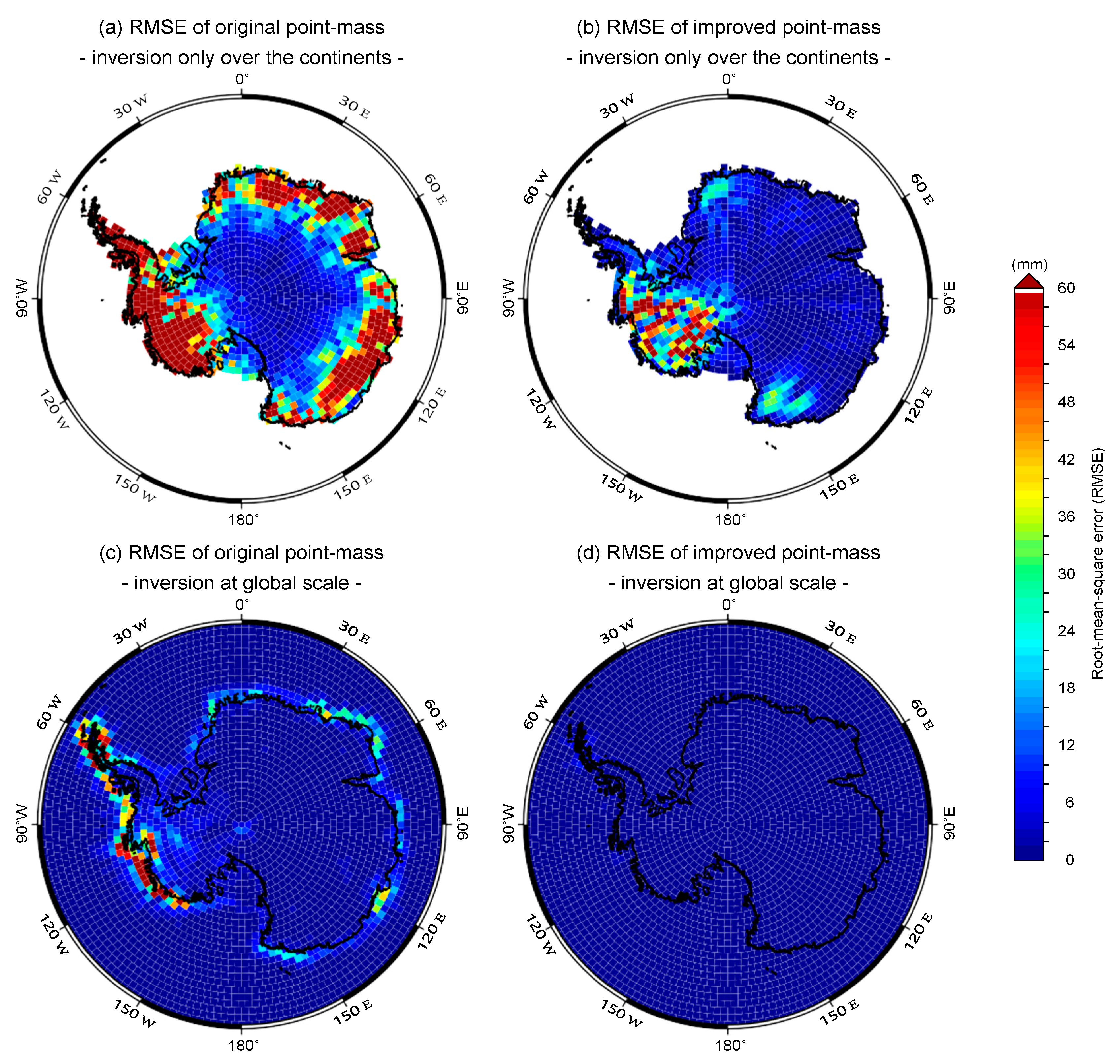
3.1. Assessment of OPM and IPM by Means of a Closed-Loop Simulation

One of the goals of this study is to validate the original point-mass (OPM) modeling since it has been identified as a viable methodology for processing GRACE Level-2 data (cf. Reference [36]) and applied in many relevant studies (e.g., References [34,35,36,37,39]). In this context, a closed-loop simulation is performed to assess the point-mass solution. In this section it is presented the evaluation of the zeroth- and third-order approximations of Equation (10) in a closed-loop scenario considering the GSFC-M e.w.h. fields as inputs.

The seasonal variations in GSFC-M e.w.h. fields from January 2003 to December 2015 (142 months, there are missing periods) were summarized in terms of the root-mean-square (RMS) of the mass changes series at each of the 41,168 equal-area cells (Figure 3a).

The monthly e.w.h. fields were used with Equation (20) to forward the respective gravitational potentials at an altitude of 500 km with a spatial resolution of $1^{\circ }$ in $\mathsf{\Delta }\phi$ and varying $\mathsf{\Delta }\lambda$ per latitude-band, totalizing 41,168 points. Figure 3b summarizes the respective gravitational potentials in terms of the RMS values. The use of the integral in Equation (20) to forward the gravitational potential at GRACE’s altitude is assumed to be an independent and superior solution for the gravitational potential regarding Equation (10). This forward modeling, which aims to find the gravitational potential at 500 km altitude given the water masses on the Earth’s surface, is essentially an upward continuation. The upward continuation works as a low-pass filter, as can be seen in Figure 3b, where the gravity field weakens with altitude, and short wavelengths are more attenuated than longer ones. Similar to Figure 3a, the spatial patterns of the gravitational potential shown in Figure 3b illustrate the long-wavelength features of the water masses, where the changes over South America and the tropical wet and dry regions of Africa remain evident. Noteworthy, the values of the gravitational potential over Greenland and West AIS are shown higher than central South America, specifically at Amazon basin. These values over West AIS are due to the ice melting rather than the seasonality due to the accumulation and oblation variations over AIS. (The simulated mass changes represented by the GSFC-M were not de-trended.)

Inverse modeling was performed to estimate the surface densities as the parameters ($\mathbf{m}$), expressed as e.w.h. $\mathsf{\Delta }r$, on the spherically approximated Earth’s surface with radius 6378 km with the gravitational potential fields at 500 km altitude taken as observations. This was performed in two different ways. First, the gravitational potential values at 41,168 bins with altitude equals 500 km were computed through Equation (20) due to the 11,930 mass change panels from GSFC-M covering only the continents (i.e., the oceans were masked out). Second, the gravitational potential values at 41,168 bins at an altitude of 500 km were also computed through Equation (20) due to the 41,168 mass change panels from GSFC-M covering whole Earth. Noteworthy, the use of GSFC-M mass changes and Equation (20) is to ensure independent observations ($\mathbf{d}$) in a closed-loop scenario to evaluate Equation (10) in its zeroth- (OPM) and third-order (IPM) approximations. Equation (10) become a linear matrix equation as $\mathbf{d}=\mathbf{G}\mathbf{m}$, where the coefficient matrix $\mathbf{G}\in {\mathbb{R}}^{n\times m}$, has a dimension of 41,168-by-11,930 considering only continents, and 41,168-by-41,168 given the entire Earth. Such a system is rank-deficient, which produces an infinite number of solutions. Consequently, the inverse problem was solved by using the Tikhonov-regularized least-squares at which the regularization parameter for each inversion was found using the L-curve criterion (see Reference [55] for details). The inversions through January 2003 to December 2015 (142 months) were performed using the respective zeroth- and third-order approximations of Equation (10), that is, OPM and IPM formulations, as the functional models. The results are summarized in Figure 4 in terms of RMS of the errors (RMSE) regarding the initial mass changes inputs.

In general, the OPM solution (zeroth-order approximation) presents larger RMSE values of the inverted masses regarding the IPM (third-order approximation), as summarized in

Table 1. Summary of quantitative statistics for the assessment of OPM (zeroth-order approximation) and IPM (third-order approximation) solutions based on a closed-loop experiment.

Domain of the Inversion	Solution	Domain of the Evaluation
		Land		Global		Antarctica
		RMSE (mm)	RSR (Unitless)	RMSE (mm)	RSR (Unitless)	RMSE (mm)	RSR (Unitless)
Land	OPM	23.82	0.29	-	-	58.94	0.52
	IPM	2.90	0.03	-	-	9.46	0.08
Global	OPM	2.41	0.03	1.68	0.04	3.83	0.03
	IPM	0.16	0.00	0.13	0.00	0.21	0.00

. The IPM solution presented an area-weighted averaged RMSE of 2.90 mm against 23.82 mm for the original point-mass (reduction of approximately 87%) considering the recovered masses over the continents (i.e., the oceans were masked out in the forward and inverse modeling). For the OPM solution, large RMSEs concentrate at the coastlines, as can be seen, for example, at the Antarctica region (Figure 4a). Such patterns are not apparent in the RMSE values of surface densities recovered by the IPM modeling (Figure 4b). Furthermore, the evaluation only over the Antarctica region presents an RMSE value of 58.94 mm and 9.46 mm for OPM and IPM solutions, respectively (Table 1). Despite the high RMSE values over Antarctica, yet the OPM presents a good performance based on the ratio of the RMSE to the standard deviation of the observed data (RSR, cf. Reference [56]). (RSR values less than 0.60 are seen as indicators of good performance as discussed in Reference [56]).

However, edge effects are apparent in the inversion targeting only the continents as seen in Figure 4a (the same holds at the global scale, which has not been shown here). In order to reduce the edge effects, it was also performed an investigation by considering the parameters covering the whole Earth, which gives a total of 41,168 parameters in comparison with the initial 11,930 parameters over the continents. The edge effects shown in Figure 4a were substantially reduced at which the occurrences of the patterns are less and with lower amplitudes, as shown in Figure 4c in the case of the OPM solution. The RMSE values changed from 23.82 mm to 2.41 mm, considering the evaluation only over the landmasses (Table 1). Nevertheless, the IPM modeling still performs better than the OPM formulation in recovering the signals with almost no noise (0.16 mm), as shown in Figure 4d. Furthermore, the weighted RMSE values considering the whole Earth are 1.68 mm and 0.13 mm for OPM and IPM solutions, respectively. The averaged (weighted) RMSE values over Antarctica presented very good performance as depicted by the RSR in Table 1 for both solutions.

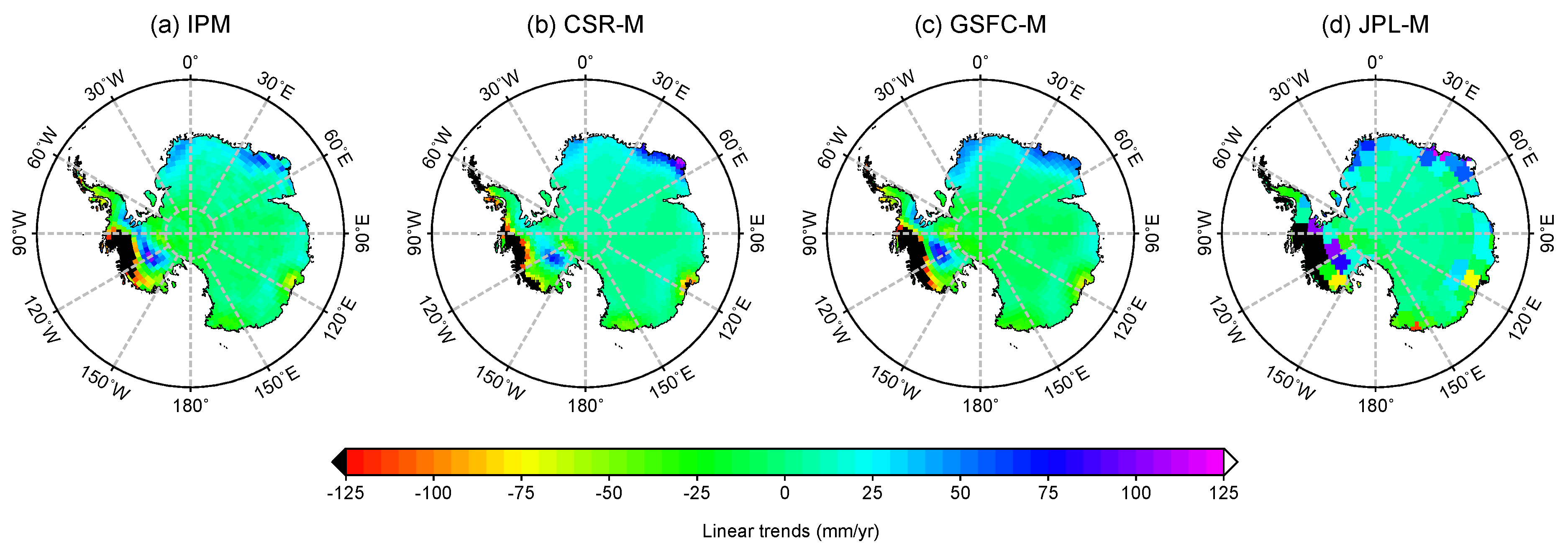
3.2. Inversion of GRACE Level-2 Data Using the IPM Modeling

The feasibility of the IPM formulation based on a closed-loop simulation showed that it delivered better results than the OPM modeling (Section 3.2). Thereby, in this section, only IPM is considered to provide a practical application as a post-processing alternative for the GRACE Level-2 product (see Figure 1). The monthly ITSG-Grace2018 solutions (Section 2.2.1) were used to synthesize the respective monthly residual gravitational potential fields from Jan 2003 to Dec 2015. Monthly regional grids of gravitational potential were synthesized at 500 km altitude with spatial resolutions of 1${}^{\circ }$-by-1${}^{\circ }$ given 64,800 bins as monthly observations. Each set of monthly fields formed the observations required in the inversion of Equation (10), in which the parameters (mass changes) were estimated. The mass changes were parametrized by the surface density values of 41,168 distributed, equal-area spherical panels, which were the unknown parameters ($\mathbf{m}$). Figure 5a shows the resulting summary of the spatial distribution of the linear trends of e.w.h. series for each equal-area panel over whole AIS. The linear trends refer to the best fit of the series considering constant, linear trend, annual, semi-annual, and 161-days components regarding the period from January 2003 to December 2015. The spatial patterns of the estimated linear trends based on the IPM and those from mascon solutions generally agree within the AIS (Figure 5). The trends from all four solutions present mass loss over the West AIS, specifically north of Ellsworth Land and Marie Byrd Land, at which JPL-M (Figure 5d) shows broader signals relative to the other solutions.

The GRACE monthly solutions can be better used at a basin- or region-level time series analysis. Hence, the areal-weighted series for the different solutions over the AIS were estimated to characterize the individual performance of the different solutions (Figure 6a). The AIS-level time series for the CSR-M and JPL-M solutions show close seasonal behaviors and long-term trends, while the GSFC-M presents the highest and lowest amplitudes characterized by a steep slope relative to the others. On the other hand, the time series for the IPM lies to a certain degree between the range of the other solutions. For instance, the linear trends of mass change series shown in Figure 6a are −5.57, −10.78, −7.45, and −7.58 mm per year (mm/year) for CSR-M, GSFC-M, JPL-M and IMP, respectively.

A multiple-comparison test [57] was considered to determining the similarities (if any) of the monthly series presented in Figure 6a. A nonparametric Kruskal-Wallis test [58] at a 95% confidence interval was applied to the monthly series of the four solutions to determine whether there were statistically significant differences among them. Figure 6b shows the box plots for the respective solutions at which their notches overlap, indicating that the actual medians of the mass changes series do not differ at 95% confidence. Subsequently, a follow-up test was conducted to identify which solution presented monthly values of mass changes resulting from a different distribution. The relative performance of the four solutions using the multiple-comparison test, based on the Tukey-Kramer procedure, indicated that there is no significant difference among the series. While the series of the four solutions are not significant different (Figure 6b), this may imply that they have the same level of accuracy over the AIS. Nevertheless, validation of the GRACE solutions in terms of e.w.h. requires independent datasets, which are not available.

However, attempts in evaluating the different GRACE solutions have been proposed based on selecting a region with minimal mass variations, like Sahara desert [7], the analysis of the de-trended and de-seasoned residuals [59], the ensemble prediction and inter-comparison analysis [60], and the noise decoupling problem [61]. The assessment suggested by Groh et al. [59] was carried out to evaluate the four time series shown in Figure 6a. Specifically, the residuals of the de-trended and de-seasoned series (already discussed) were smoothed using a 13-month moving average, and the differences between both (original and filtered residuals) as shown in Figure 6c were used to assess the noise level of the solutions. The high-pass filtered residuals shown in Figure 6c present low correlation (autocorrelation). This indicates that more noise dominates the high-pass filtered residuals of the respective solutions. Figure 6d shows the box plots summarizing the high-pass filtered residuals at which the RMSEs are 5.02, 6.05, 5.81, and 5.77 mm, for CSR-M, GSFC-M, JPL-M, and IPM, respectively. That is, IPM ranks second best among the four solutions.

4. Discussion

Two of the main goals of this experiment were (i) investigating the point-mass modeling, and (ii) proposing an improved alternative solution. Thus, a refinement for the so-called point-mass solution was forwarded, which considers terms neglected in the integration of the surface integral (see Equation (4)) for the calculation of the gravitational potential. Because the surface integral cannot be solved in closed analytical form, a Taylor series expansion to its integrand was applied. By evaluating the series at a point equivalent to the geometric center ($Q_0$) of the spherical panels, the number of non-vanishing terms was reduced because only even terms remained after subsequent integration as shown by Equation (11). Furthermore, the zeroth-order term of the series corresponds to the OPM solution, and the additional higher-order terms represent the deviation of a panel from a point-mass. The results summarized in Table 1 show that the OPM modeling is within the range of the uncertainties expected for GRACE-derived e.w.h. fields. For example, Scanlon et al. [27] have reported uncertainties of GRACE-derived e.w.h. in the range of 5 to 40 mm for river basins larger than 100 × 10${}^3$ km${}^2$ (for smaller basins, these values are slightly higher). Groh et al. [59] have estimated uncertainties ranging from approx. 5.9 to 8.1 mm for AIS (considering AIS’s surface area as approx. 12 × 10${}^6$ km${}^2$). Although the differences in the period and release of the GRACE Level-2 datasets between the studies, the uncertainties of GRACE solutions seem to be less than 10 mm at AIS. However, artifacts can be detected in the global map of the RMSEs (not shown here) of the inverted mass changes regarding OPM. For instance, Figure 4a shows a pattern of the RMSEs where large values concentrate along the AIS’s coastlines (the same holds for all landmasses).

As the spatial patterns might be a consequence of edge effects in the inversion, computations considering parameters covering the whole Earth reduced the edge effects to a certain extent. For instance, the RMSE reduced in approximately 90% (Table 1) while solving the inverse problem using the OPM modeling considering the edge effects. Furthermore, considering higher-order terms in Equation (10), improve the point-mass (i.e., IPM) approach. For instance, considering terms up to third-order reduced the edge effects (Figure 4) as well as the RMSE values (Table 1). In this study, it was considered only a third-order expansion of the surface integral (Equation (10)), and the contribution of higher-order terms (if any) was not investigated. Nevertheless, analyzing the remainder of the series expansion of the kernel given by Equation (5), performed at the Appendix B (see Equation (A13)), it is shown that the relative error due to the fourth-order approximation in terms of forwarded gravitational potential is less than 0.01%. (These figures are approximated 0.10% and 0.02% for the zeroth- and second-order approximations, respectively.) Therefore, objectives (i) and (ii) proposed in Section 1 were met. Moreover, with or without accounting for edge effects, the IPM solution went one better than the OPM solution (Figure 4). The contribution of this exercise lies in the regional application of OPM modeling, for example, for estimating mass changes over Antarctica, which requires adding buffer zones in the inversion, which has not been discussed in the previous studies (e.g., Reference [38]).

Consequently, the IPM modeling provides an alternative procedure to recover AIS’s mass changes using synthesized gravitational potential fields projected at GRACE’s altitude as wished-for in objective (iii). Thus, in Section 3.2, it is presented the mass changes over AIS based only on IPM. At this stage, OPM was not considered in the inversion of Level-2 data since the comparison between both mass parametrizations would be necessary to apply a low-pass filter to the models in order to make them spectrally consistent with the synthesized residual gravitational potentials, which are band-limited up to d/o 120. This is important since OPM and IPM parametrizations could bias the short wavelengths of the estimated mass changes in different ways. It will be investigated in a follow-up study. In any case, the preliminary results depicted in Section 3.2 indicate that IPM ranks the second best with an RMSE of 5.77 mm. However, if CSR mascon solution (CSR-M) provides slightly better results over AIS (see Figure 6d), why should one consider the IPM modeling (the same holds for the OPM modeling) as a GRACE processing approach? Andrews et al. [26] and Scanlon et al. [27], among other authors, have shown that unconstrained mascon and unfiltered spherical harmonic solutions have the same variances at different frequencies. This might indicate that both solutions provide the same results for inverted mass changes, in which the differences are consequences of the constrain in the mascon solutions and filtering in the spherical harmonic solutions. Generally, when the whole time series of GRACE raw data are reprocessed in order to implement new corrections and/or reductions based on improved de-aliasing products, the first friendly solutions available to the public are Level-2 data. However, there is typically a large latency before new releases of corresponding mascon solutions are provided. Thus, as the IPM method is based directly on Level-2 data, users immediately benefit from new releases to obtain improvements in the estimated mass changes.

Furthermore, while there are three centers that provide mascon solutions to the public [15,20,25], there are numerous research groups (see, e.g., References [3,4,5,6,7,8,9,10,11,12,13,14]) from three continents that generate Level-2 data based on different approaches and methods in order to make the most out of the GRACE measurements. Additionally, the Level-2 data from the measurements of the state-of-art satellite gravimetry GRACE Follow-On (GRACE-FO) is already available, extending the legacy of the former GRACE mission. Mascon solutions based on GRACE-FO might show up anytime, and, meanwhile, the users can use GRACE-FO Level-2 data in the framework of IPM modeling (or the OPM if considered the edge effects) as a viable processing methodology akin to mascon solutions as shown for AIS (Figure 6d). The consistencies among the products are also depicted in the overall mass loss of AIS over the period from 2003–2015. The rates of −5.57, −10.78, −7.45, and −7.58 mm per year (mm/yr) for CSR-M, GSFC-M, JPL-M, and IMP, respectively are seen from Figure 6a. These values agree with the linear trends estimated by, for example, Groh et al. [59], who have estimated figures about −8.0 mm/yr.

The mass change estimations over AIS considered only the Level-2 dataset represented by the ITSG-Grace2018 solution. The reason for this was that the assessment of ITSG-Grace2018 conducted by Kvas et al. [8] has shown up 46% lower noise level than the Release 06 solutions produced by CSR, GFZ, and JPL over the quite ocean areas. Furthermore, these authors have investigated the performance of ITSG-Grace2018 over 33 river basins (basins at which the noise level does not affect the signal), and it has been reported that ITSG-Grace2018 exhibits the same signal content like CSR, GFZ, and JPL with variability at the range of ±2 mm. This indicates that the choice of one or another solution would not impact the finds in Section 3.2 up to a certain point. Nevertheless, the inversion using all (or most of them) Level-2 solutions produced by other processing centers and institutions could lead to a higher generalization of the results. Although this is a small study focusing on the entire AIS, the results in Section 3.2 cannot be generalized to the sub-domains of AIS, for example, West AIS (or other regions). Hence, a global assessment of the inversion of mass changes parameterized by IPM still necessary. To this end, the inversion at a global scale using Tikhonov-regularized least-squares may be computationally expensive for the most of users since it depends on the computation of the decomposition matrices. Solutions to the least-squares problem may be calculated very easily using conjugated gradient-like methods on the normal equations (e.g., Reference [62]). Alternatively, one could consider a regional application at which the parameters conveying the target region (or basin) plus a buffer zone could be estimated. Although the results presented here are based on Level-2 data, the IPM can be used in the same fashion way to invert Level-1b data as, for example, the approach used by JPL-M (cf. Reference [15]).

5. Conclusions

In this paper, it was investigated the overall performance of the original point-mass (OPM) formalism and proposed an improvement (IPM) as well. For instance, a closed-loop simulation using inverse modeling showed that the IPM solution outperformed the results based on OPM modeling at global and regional scales. The OPM is more susceptible to the edge effects in the inversion than IPM, which are concentrated along the coastlines. For example, the RMSE values along the coastal regions are reduced to a large extent while parametrizing the surface densities with IPM modeling. That is, considering the inversion over the entire Earth, it upgrades the OPM’s performance to the level of that of the IPM solution. This means that the application of OPM requires an extended area beyond the target region’s domain (for example, five arc-degrees). Regarding the AIS’s mass changes, the overall patterns of the linear trends of GRACE-era mass changes considering the IPM modeling were estimated at which a linear trend of −7.58 mm/year are in agreement with those of the mascon solutions (CSR-M, GSFC-M, and JPL-M). Noise assessment of the IPM solution has shown RMSE values at the same level as the mascon solutions. Therefore, it is concluded that all the variabilities of the different GRACE solutions analyzed here indicate the level of noise in GRACE data over AIS. Albeit mascon solutions are available for the public and being a friendly product for the most of users, the IPM associated with synthesized potential from Level-2 data can be seen as a fast and quick means to assess mass changes at regional or global scales.

References

1. Tapley, B.D.; Bettadpur, S.; Ries, J.C.; Thompson, P.F.; Watkins, M.M. GRACE measurements of mass variability in the Earth system. Science 2004, 305, 503–505. [Google Scholar] [CrossRef] [Green Version]
2. Tapley, B.D.; Watkins, M.M.; Flechtner, F.; Reigber, C.; Bettadpur, S.; Rodell, M.; Sasgen, I.; Famiglietti, J.S.; Landerer, F.W.; Chambers, D.P.; et al. Contributions of GRACE to understanding climate change. Nat. Clim. Chang. 2019, 9, 358–369. [Google Scholar] [CrossRef]
3. Bettadpur, S. UTCSR Level-2 Processing Standards Document: For Level-2 Product Release 0006; Center for Space Research, The University of Texas at Austin: Austin, TX, USA, 2018. [Google Scholar]
4. Watkins, M.M.; Yuan, D.N. JPL Level-2 Processing Standards Document for Level-2 Product Release 05.1; Jet Propulsion Laboratory–JPL, California Institute of Technology: Pasadena, CA, USA, 2014. [Google Scholar]
5. Dahle, C.; Flechtner, F.; Murböck, M.; Michalak, G.; Neumayer, K.; Abrykosov, O.; Reinhold, A.; König, R. GRACE 327–743 (Gravity Recovery and Climate Experiment): GFZ Level-2 Processing Standards Document for Level-2 Product Release 06 (Rev. 1.0, 26 October 2018); Scientific Technical Report str—Data; GFZ German Research Centre for Geosciences: Potsdam, Germany, 2018. [Google Scholar] [CrossRef]
6. Lemoine, J.; Bruinsma, S.; Gegout, P.; Biancale, R.; Bourgogne, S. Release 3 of the GRACE gravity solutions from CNES/GRGS. In Geophysical Research Abstracts; European Geoscience Union: Vienna, Austria, 2013; Volume 15, p. EGU2013-11123. [Google Scholar]
7. Liu, X.; Ditmar, P.; Siemes, C.; Slobbe, D.C.; Revtova, E.; Klees, R.; Riva, R.; Zhao, Q. DEOS Mass Transport model (DMT-1) based on GRACE satellite data: Methodology and validation. Geophys. J. Int. 2010, 181, 769–788. [Google Scholar] [CrossRef] [Green Version]
8. Kvas, A.; Behzadpour, S.; Ellmer, M.; Klinger, B.; Strasser, S.; Zehentner, N.; Mayer-Gürr, T. ITSG-Grace2018: Overview and Evaluation of a New GRACE-Only Gravity Field Time Series. J. Geophys. Res. Solid Earth 2019, 124, 9332–9344. [Google Scholar] [CrossRef] [Green Version]
9. Meyer, U.; Jäggi, A.; Jean, Y.; Beutler, G. AIUB-RL02: An improved time-series of monthly gravity fields from GRACE data. Geophys. J. Int. 2016, 205, 1196–1207. [Google Scholar] [CrossRef] [Green Version]
10. Chen, Q.; Shen, Y.; Zhang, X.; Hsu, H.; Chen, W.; Ju, X.; Lou, L. Monthly gravity field models derived from GRACE Level 1B data using a modified short-arc approach. J. Geophys. Res. Solid Earth 2015, 120, 1804–1819. [Google Scholar] [CrossRef]
11. Naeimi, M.; Koch, I.; Khami, A.; Flury, J. IfE monthly gravity field solutions using the variational equations. In Geophysical Research Abstracts; European Geoscience Union: Vienna, Austria, 2018; Volume 20. [Google Scholar]
12. Chen, W.; Luo, J.; Ray, J.; Yu, N.; Li, J.C. Multiple-data-based monthly geopotential model set LDCmgm90. Sci. Data 2019, 6, 228. [Google Scholar] [CrossRef] [Green Version]
13. Jean, Y.; Meyer, U.; Jäggi, A. Combination of GRACE monthly gravity field solutions from different processing strategies. J. Geod. 2018, 92, 1313–1328. [Google Scholar] [CrossRef] [Green Version]
14. Meyer, U.; Jean, Y.; Kvas, A.; Dahle, C.; Lemoine, J.M.; Jäggi, A. Combination of GRACE monthly gravity fields on the normal equation level. J. Geod. 2019, 93, 1645–1658. [Google Scholar] [CrossRef] [Green Version]
15. Watkins, M.M.; Wiese, D.N.; Yuan, D.N.; Boening, C.; Landerer, F.W. Improved methods for observing Earth’s time variable mass distribution with GRACE using spherical cap mascons. J. Geophys. Res. Solid Earth 2015, 120, 2648–2671. [Google Scholar] [CrossRef]
16. Swenson, S.; Wahr, J. Post-processing removal of correlated errors in GRACE data. Geophys. Res. Lett. 2006, 33, L08402. [Google Scholar] [CrossRef]
17. Swenson, S.; Wahr, J. Methods for inferring regional surface-mass anomalies from Gravity Recovery and Climate Experiment (GRACE) measurements of time-variable gravity. J. Geophys. Res. 2002, 107, 2193. [Google Scholar] [CrossRef] [Green Version]
18. Kusche, J. Approximate decorrelation and non–isotropic smoothing of time-variable GRACE-type gravity field models. J. Geod. 2007, 81, 733–749. [Google Scholar] [CrossRef] [Green Version]
19. Rowlands, D.D.; Luthcke, S.B.; Klosko, S.M.; Lemoine, F.G.R.; Chinn, D.S.; McCarthy, J.J.; Cox, C.M.; Anderson, O.B. Resolving mass flux at high spatial and temporal resolution using GRACE intersatellite measurements. Geophys. Res. Lett. 2005, 32, L04310. [Google Scholar] [CrossRef]
20. Luthcke, S.B.; Zwally, H.J.; Abdalati, W.; Rowlands, D.D.; Ray, R.D.; Nerem, R.S.; Lemoine, F.G.; McCarthy, J.J.; Chinn, D.S. Recent Greenland ice mass loss by drainage system from satellite gravity observations. Science 2006, 314, 1286–1289. [Google Scholar] [CrossRef] [PubMed] [Green Version]
21. Klees, R.; Liu, X.; Wittwer, T.; Gunter, B.C.; Revtova, E.A.; Tenzer, R.; Ditmar, P.; Winsemius, H.C.; Savenije, H.H.G. A Comparison of Global and Regional GRACE Models for Land Hydrology. Surv. Geophys. 2008, 29, 335–359. [Google Scholar] [CrossRef] [Green Version]
22. Rowlands, D.D.; Luthcke, S.B.; McCarthy, J.J.; Klosko, S.M.; Chinn, D.S.; Lemoine, F.G.; Boy, J.P.; Sabaka, T.J. Global mass flux solutions from GRACE: A comparison of parameter estimation strategies—Mass concentrations versus Stokes coefficients. J. Geophys. Res. 2010, 115, B01403. [Google Scholar] [CrossRef]
23. Sabaka, T.J.; Rowlands, D.D.; Luthcke, S.B.; Boy, J.P. Improving global mass flux solutions from Gravity Recovery and Climate Experiment (GRACE) through forward modeling and continuous time correlation. J. Geophys. Res. 2010, 115, 1–20. [Google Scholar] [CrossRef]
24. Luthcke, S.B.; Sabaka, T.; Loomis, B.; Arendt, A.; McCarthy, J.; Camp, J. Antarctica, Greenland and Gulf of Alaska land-ice evolution from an iterated GRACE global mascon solution. J. Glaciol. 2013, 59, 613–631. [Google Scholar] [CrossRef]
25. Save, H.; Bettadpur, S.; Tapley, B.D. High-resolution CSR GRACE RL05 mascons. J. Geophys. Res. Solid Earth 2016, 121, 7547–7569. [Google Scholar] [CrossRef]
26. Andrews, S.B.; Moore, P.; King, M.A. Mass change from GRACE: A simulated comparison of Level-1B analysis techniques. Geophys. J. Int. 2014, 200, 503–518. [Google Scholar] [CrossRef] [Green Version]
27. Scanlon, B.R.; Zhang, Z.; Save, H.; Wiese, D.N.; Landerer, F.W.; Long, D.; Longuevergne, L.; Chen, J. Global evaluation of new GRACE mascon products for hydrologic applications. Water Resour. Res. 2016, 52, 9412–9429. [Google Scholar] [CrossRef]
28. Wahr, J.; Molenaar, M.; Bryan, F. Time variability of the Earth’s gravity field: Hydrological and oceanic effects and their possible detection using GRACE. J. Geophys. Res. 1998, 103, 30205. [Google Scholar] [CrossRef]
29. Klees, R.; Zapreeva, E.A.; Winsemius, H.C.; Savenije, H.H.G. The bias in GRACE estimates of continental water storage variations. Hydrol. Earth Syst. Sci. 2007, 11, 1227–1241. [Google Scholar] [CrossRef] [Green Version]
30. Tiwari, V.M.; Wahr, J.; Swenson, S. Dwindling groundwater resources in northern India, from satellite gravity observations. Geophys. Res. Lett. 2009, 36, L18401. [Google Scholar] [CrossRef] [Green Version]
31. Jacob, T.; Wahr, J.; Pfeffer, W.T.; Swenson, S. Recent contributions of glaciers and ice caps to sea level rise. Nature 2012, 482, 514–518. [Google Scholar] [CrossRef]
32. Schrama, E.J.; Wouters, B.; Rietbroek, R. A mascon approach to assess ice sheet and glacier mass balances and their uncertainties from GRACE data. J. Geophys. Res. Solid Earth 2014, 119, 6048–6066. [Google Scholar] [CrossRef]
33. Ran, J.; Ditmar, P.; Klees, R.; Farahani, H.H. Statistically optimal estimation of Greenland Ice Sheet mass variations from GRACE monthly solutions using an improved mascon approach. J. Geod. 2018, 92, 299–319. [Google Scholar] [CrossRef] [Green Version]
34. Forsberg, R.; Reeh, N. Mass change of the Greenland Ice Sheet from GRACE. In Gravity Field of the Earth—1st Meeting of the International Gravity Field Service; Dergisi, H., Ed.; Springer: Berlin/Heidelberg, Germany, 2007; pp. 1–5. [Google Scholar]
35. Sørensen, L.S.; Forsberg, R. Greenland Ice Sheet Mass Loss from GRACE Monthly Models. In Gravity, Geoid and Earth Observation; Mertikas, S.P., Ed.; Springer: Berlin/Heidelberg, Germany, 2010; pp. 527–532. [Google Scholar]
36. Baur, O.; Sneeuw, N. Assessing Greenland ice mass loss by means of point-mass modeling: A viable methodology. J. Geod. 2011, 85, 607–615. [Google Scholar] [CrossRef]
37. Barletta, V.R.; Sørensen, L.S.; Forsberg, R. Scatter of mass changes estimates at basin scale for Greenland and Antarctica. Cryosphere 2013, 7, 1411–1432. [Google Scholar] [CrossRef] [Green Version]
38. Forsberg, R.; Sørensen, L.; Simonsen, S. Greenland and Antarctica Ice Sheet Mass Changes and Effects on Global Sea Level. Surv. Geophys. 2017, 38, 89–104. [Google Scholar] [CrossRef] [Green Version]
39. Ferreira, V.; Yong, B.; Tourian, M.; Ndehedehe, C.; Shen, Z.; Seitz, K.; Dannouf, R. Characterization of the hydro-geological regime of Yangtze River basin using remotely-sensed and modeled products. Sci. Total Environ. 2020, 718, 137354. [Google Scholar] [CrossRef] [Green Version]
40. Heck, B.; Seitz, K. A comparison of the tesseroid, prism and point-mass approaches for mass reductions in gravity field modelling. J. Geod. 2007, 81, 121–136. [Google Scholar] [CrossRef]
41. Mohr, P.J.; Newell, D.B.; Taylor, B.N. CODATA Recommended Values of the Fundamental Physical Constants: 2014. J. Phys. Chem. Ref. Data 2016, 45, 043102. [Google Scholar] [CrossRef] [Green Version]
42. Chao, B.F. Caveats on the equivalent water thickness and surface mascon solutions derived from the GRACE satellite-observed time-variable gravity. J. Geod. 2016, 90, 807–813. [Google Scholar] [CrossRef]
43. Wild-Pfeiffer, F. A comparison of different mass elements for use in gravity gradiometry. J. Geod. 2008, 82, 637–653. [Google Scholar] [CrossRef]
44. Grombein, T.; Seitz, K.; Heck, B. Optimized formulas for the gravitational field of a tesseroid. J. Geod. 2013, 87, 645–660. [Google Scholar] [CrossRef]
45. Grombein, T.; Seitz, K.; Awange, J.L.; Heck, B. Detection of hydrological mass variations by means of an inverse tesseroid approach. In Geophysical Research Abstracts; European Geoscience Union: Vienna, Austria, 2012; Volume 14, p. EGU2012-7548. [Google Scholar]
46. Mayer-Gürr, T.; Behzadpur, S.; Ellmer, M.; Kvas, A.; Klinger, B.; Strasser, S.; Zehentner, N. ITSG-Grace2018—Monthly, Daily and Static Gravity Field Solutions from GRACE. Available online: https://www.tugraz.at/institute/ifg/downloads/gravity-field-models/itsg-grace2018/ (accessed on 13 March 2020).
47. Swenson, S.; Chambers, D.; Wahr, J. Estimating geocenter variations from a combination of GRACE and ocean model output. J. Geophys. Res. 2008, 113, 1–12. [Google Scholar] [CrossRef] [Green Version]
48. Cheng, M.; Tapley, B.D. Variations in the Earth’s oblateness during the past 28 years. J. Geophys. Res. 2004, 109, B09402. [Google Scholar] [CrossRef]
49. A, G.; Wahr, J.; Zhong, S. Computations of the viscoelastic response of a 3-D compressible Earth to surface loading: An application to Glacial Isostatic Adjustment in Antarctica and Canada. Geophys. J. Int. 2013, 192, 557–572. [Google Scholar] [CrossRef]
50. Save, H. CSR GRACE RL06 Mascon Solutions. Texas Data Repository Dataverse, V1. Available online: https://disc.gsfc.nasa.gov/datasets/GLDAS_NOAH10_M_V2.1/summary (accessed on 23 October 2019).
51. Wiese, D.N.; Landerer, F.W.; Watkins, M.M. Quantifying and reducing leakage errors in the JPL RL05M GRACE mascon solution. Water Resour. Res. 2016, 52, 7490–7502. [Google Scholar] [CrossRef]
52. Wiese, D.N.; Yuan, D.N.; Boening, C.; Landerer, F.W.; Watkins, M.M. JPL GRACE Mascon Ocean, Ice, and Hydrology Equivalent Water Height Release 06 Coastal Resolution Improvement (CRI) Filtered Version 1.0. Ver. 1.0. Available online: https://grace.jpl.nasa.gov/data/get-data/jpl_global_mascons/ (accessed on 16 March 2019).
53. Rignot, E.; Jacobs, S.; Mouginot, J.; Scheuchl, B. Ice-Shelf Melting Around Antarctica. Science 2013, 341, 266–270. [Google Scholar] [CrossRef] [Green Version]
54. Mouginot, J.; Scheuchl, B.; Rignot, E. MEaSUREs Antarctic Boundaries for IPY 2007–2009 from Satellite Radar, Version 2. Available online: https://nsidc.org/data/nsidc-0709 (accessed on 12 July 2020).
55. Hansen, P.C. The L-Curve and its Use in the Numerical Treatment of Inverse Problems. In Computational Inverse Problems in Electrocardiology, Advances in Computational Bioengineering; Johnston, P., Ed.; WIT Press: Southampton, UK, 2000; Volume 4, pp. 119–142. [Google Scholar]
56. Moriasi, D.N.; Arnold, J.G.; Liew, M.W.V.; Bingner, R.L.; Harmel, R.D.; Veith, T.L. Model Evaluation Guidelines for Systematic Quantification of Accuracy in Watershed Simulations. Trans. ASABE 2007, 50, 885–900. [Google Scholar] [CrossRef]
57. Hochberg, Y.; Tamhane, A.C. Multiple Comparison Procedures; Wiley Series in Probability and Statistics; John Wiley & Sons, Inc.: Hoboken, NJ, USA, 1987. [Google Scholar] [CrossRef] [Green Version]
58. Kruskal, W.H.; Wallis, W.A. Use of Ranks in One-Criterion Variance Analysis. J. Am. Stat. Assoc. 1952, 47, 583–621. [Google Scholar] [CrossRef]
59. Groh, A.; Horwath, M.; Horvath, A.; Meister, R.; Sørensen, L.S.; Barletta, V.R.; Forsberg, R.; Wouters, B.; Ditmar, P.; Ran, J.; et al. Evaluating GRACE Mass Change Time Series for the Antarctic and Greenland Ice Sheet–Methods and Results. Geosciences 2019, 9, 415. [Google Scholar] [CrossRef] [Green Version]
60. Sakumura, C.; Bettadpur, S.; Bruinsma, S. Ensemble prediction and intercomparison analysis of GRACE time-variable gravity field models. Geophys. Res. Lett. 2014, 41, 1389–1397. [Google Scholar] [CrossRef]
61. Ferreira, V.G.; Montecino, H.D.C.; Yakubu, C.I.; Heck, B. Uncertainties of the Gravity Recovery and Climate Experiment time-variable gravity-field solutions based on three-cornered hat method. J. Appl. Remote. Sens. 2016, 10, 015015. [Google Scholar] [CrossRef]
62. Paige, C.C.; Saunders, M.A. LSQR: An Algorithm for Sparse Linear Equations and Sparse Least Squares. ACM Trans. Math. Softw. 2002, 8, 43–71. [Google Scholar] [CrossRef]
63. Bronstein, I.; Semendjajew, K.; Musiol, G.; Mühlig, H. Taschenbuch Der Mathematik, 4th ed.; Verlag Harri Deutsch: Frankfurt am Main, Germany, 1999. [Google Scholar]
Figure 1. Flow chart showing the experiment used for assessing the original (zeroth-order) and improved point-mass (third-order) solutions as per Equation (10) as well as a study case over Antarctica using GRACE Level-2 data as given by ITSG-Grace2018.
Remotesensing 12 03197 g001
Figure 2. The map shows the division of the Antarctica Ice Sheet (AIS) into the ice front (defines the coastlines) and grounding line (defines the landmasses) with the limits established by Rignot et al. [53]. The AIS base map also shows the partitioning of the sphere into equal-area spherical panels used in GSFC-M as defined by Luthcke et al. [24], in which the respective geometrical centers (red circles) depict the Taylor points Q 0 . The insert illustrates the geometry of an individual equal-area spherical panel in view of the equations presented in Section 2.1.1 and Section 2.1.2.
Remotesensing 12 03197 g002
Figure 3. (a) Spatial patterns of the root-mean-square (RMS) of the series of each one of the 41,168 equivalent water height panels from GSFC-M based on the period of January 2003 to December 2015. (b) Spatial patterns of the RMS of the forwarded gravitational potential at 500 km altitude according to the radial integral in Equation (20) using the GSFC-M monthly fields of equivalent water height.
Remotesensing 12 03197 g003
Figure 4. Root-mean-square errors (RMSEs) between the input mass changes from GSFC-M and those inverted from the OPM and IPM solutions over Antarctica. The panels (a,b) shows the RMSE regarding the recovering of mass changes only over the continents for OPM and IPM solutions, respectively. Similarly, to panels (a,b), panels (c,d) show the summary considering the results of the inversion accounting for a global set of mass changes.
Remotesensing 12 03197 g004
Figure 5. Linear trends derived from the mass changes referring to the best fit of the series considering constant, linear trend, annual, semi-annual, and 161-days components regarding the period from January 2003 to December 2015. Panels (ad) show results based on improved point-mass (IPM) and mascon solutions from CSR (CSR-M), GSFC (GSFC-M), and JPL (JPL-M), respectively.
Remotesensing 12 03197 g005
Figure 6. (a) The areal-weighted average time series of mass changes for the AIS for the different solutions expressed as equivalent water height (e.w.h.) in mm. (b) The box plots summaries of e.w.h. series in panel (a) at which the whiskers indicate the maximum and minimum range of e.w.h. (c) Time series of the error noise defined as the residuals of the de-trended and de-seasoned series minus low-pass filtered residuals (i.e., the high-pass filtered residuals). (d) The same as panel (b), however, for the error noises. The boxes show the interquartile (first and third quartile) ranges of variation of the values, the segments inside the respective boxes sow the median of the values, and the crosses indicate the outliers.
Remotesensing 12 03197 g006