Improving the Classification Accuracy of Annual Crops Using Time Series of Temperature and Vegetation Indices

Abstract

Accurate cropland classification is important for agricultural monitoring and related decision-making. The commonly used input spectral features for classification cannot be employed to effectively distinguish crops that have similar spectro-temporal features. This study attempted to improve the classification accuracy of crops using both the thermal feature, i.e., the land surface temperature (LST), and the spectral feature, i.e., the normalized difference vegetation index (NDVI), for classification. To amplify the temperature differences between the crops, a temperature index, namely, the modified land surface temperature index (mLSTI) was built using the LST. The mLSTI was calculated by subtracting the average LST of an image from the LST of each pixel. To study the adaptability of the proposed method to different areas, three study areas were selected. A comparison of the classification results obtained using the NDVI time series and NDVI + mLSTI time series showed that for long time series from June to November, the classification accuracy when using the mLSTI and NDVI time series was higher (85.6% for study area 1 in California, 96.3% for area 2 in Kansas, and 91.2% for area 3 in Texas) than that when using the NDVI time series alone (82.0% for area 1, 94.7% for area 2, and 90.9% for area 3); the same was true in most of the cases when using the shorter time series. With the addition of the mLSTI time series, the shorter time series achieved higher classification accuracy, which is beneficial for timely crop identification. The sorghum and soybean crops, which exhibit similar NDVI feature curves in this study, could be better distinguished by adding the mLSTI time series. The results demonstrated that the classification accuracy of crops can be improved by adding mLSTI long time series, particularly for distinguishing crops with similar NDVI characteristics in a given study area.

1. Introduction

Early studies used spectral features of single-date remote sensing images for the classification of crops. However, different crops may have similar spectral attributes in a given time period [1]; therefore, it is not always possible to capture sufficient differences for classification using a single-date image [2]. Different crops can be best discriminated at different stages; consequently, multi-temporal images have been widely used in crop classification studies [3,4,5,6]. Vieira et al. studied the spectro-temporal response for the multi-temporal classification of agricultural crops and found that multi-temporal images yield better classification accuracy than single-date images [7]. Zhang et al. investigated the effectiveness of multi-temporal images for crop identification and found that multi-temporal Landsat data can help discriminate crops in regions with high farmland fragmentation [8]. Kussul et al. studied regional-scale crop mapping using multi-temporal satellite imagery [9]. Celik et al. identified cotton and corn using multi-temporal SPOT6 normalized difference vegetation index (NDVI) images [10]. Further research showed that the time series of multi-temporal images arranged in a time sequence during growth can effectively reflect the phenological characteristics of crops, and classification based on such a time series can yield better results [11,12,13,14,15,16]. For example, using the MODIS time series, Conrad et al. improved the crop classification accuracy in Central Asian irrigation systems by 6–7% [17]. However, some issues remain unresolved. For example, using all the images of the entire growing season for crop-type mapping cannot support timely crop management at the early stages of crop growth [18]. Moreover, some crops have similar spectro-temporal changes, which affect the ability to use the spectrum features for classification [19]. Therefore, it is necessary to develop an approach using shorter time series to attain a higher classification accuracy and to better distinguish crops that exhibit similar spectro-temporal features.

Studies suggest that there are differences between the evapotranspiration of different plant types during different development stages [20] and that the evapotranspiration of crops is influenced by crop species [21]. When energy is consumed for evaporating water, the canopy temperature decreases [22], and high rates of evapotranspiration can result in the cooling of the canopy below the ambient air temperature [23]. Meier and Scherer estimated the spatio-temporal variability in the canopy temperature and concluded that the canopy temperature of urban trees depends on species-specific properties [24]. Blum et al. discovered that the canopy temperature is related to the land surface temperature (LST) in places where canopy covers most of the surface [25]. Considering the differences in the canopy temperature between different plant species and the correlation between canopy temperature and LST, this paper proposes a new approach wherein the LST is incorporated to improve the accuracy of crop classification.

In this study, we first analyzed whether incorporating a modified land surface temperature index (mLSTI) could improve the classification accuracy and its effect on timely crop identification. Subsequently, we studied the effect of adding mLSTI time series on differentiating crops with similar NDVI characteristics. Finally, we analyzed the reasons for varying accuracy after adding mLSTI.

2. Materials and Methods

2.1. Study Area

To study the feasibility and adaptability of the proposed method, we selected three study areas in this study. Firstly, we selected an area in Kansas in the central United States as the study area because it is known as an agriculturally-dominated state with diverse crop types and large crop areas. Secondly, in order to study the applicability of this method to different regions and to different crop types, we chose a study area in Texas, which is located in a belt of different crops and in California, which is particularly rich in agricultural crop varieties. Thus, study area 1 is in California, USA (Figure 1a), study area 2 is in Kansas, USA (Figure 1b), and study area 3 is in Texas, USA (Figure 1c). Figure 1 shows the latitude and longitude coordinates of the study areas. The images in Figure 1c are Landsat 8 satellite images of the three study areas that were taken in July of different years.

Table 1. Average temperature of the study areas.

	Average Temperature of Study Area 1 (°C)	Average Temperature of Study Area 2 (°C)	Average Temperature of Study Area 3 (°C)
June	24.7	25.1	23
July	28.0	26.5	26.1
August	27.1	24.5	27.5
September	23.7	21.4	23.9
October	18.7	16.0	11.8
November	14.0	9.1	6.2

lists the monthly average temperatures of the study areas. Crops that cover more than 1% of the study area are considered target crops. The target crops in study area 1 are winter wheat, grape, alfalfa, and almond [26]. The target crops in study area 2 are corn, sorghum, soybeans, winter wheat, and alfalfa [27]. The target crops in study area 3 are corn, cotton, sorghum, and winter wheat [28].

2.2. Data

The data used to calculate the features included the Landsat 7 surface reflectance product, Landsat 8 surface reflectance product, and the LST product. The National Cropland Data Layer (CDL) from the United States Department of Agriculture was used as the crop-type ground truth data. To study the adaptability of the proposed method in different years, we selected data from different years for the different study areas. The crop season in the study area is from April to November. Considering the time of planting and unearthing crops, we selected images from June to November. The dates of the cloud-free Landsat images taken during the growing period are listed in

Table 2. Date of images used in the study area.

	Study Area 1 (2017) (WRS Path 43, Rows 34)	Study Area 2 (2016) (WRS Path 29, Rows 33)	Study Area 3 (2019) (WRS Path 30, Rows 36)
June	23th	2nd	26th
July	25th	20th	4th
August	26th	21th	29th
September	11th	6th	14th
October	13th	8th	8th
November	14th	25th	9th

.

Landsat 7 Collection 2 surface reflectance products are generated at 30 m spatial resolution on a Universal Transverse Mercator (UTM) and can be downloaded from EarthExplorer (https://earthexplorer.usgs.gov/). The Landsat 8 surface reflectance product is generated at a spatial resolution of 30 m and is available at LandsatLook Viewer (https://landsatlook.usgs.gov/) [29]. The LST data came from the Landsat Provisional Surface Temperature product, which is included in the U.S. Landsat Analysis Ready Data (ARD) product bundle and is available for download at EarthExplorer. The data were processed to a spatial resolution of 30 m in the Albers equal area (AEA) projection using World Geodetic System 1984 (WGS84) datum [30,31].

The CDL, which is a raster, geo-referenced, crop-specific land cover data layer with a ground resolution of 30 m, is widely accepted as a crop-type reference data layer in crop classification studies [32,33,34,35]. The CDL program was developed by the US Department of Agriculture (USDA), National Agricultural Statistics Service (NASS) [36]. We randomly selected training and validation data from the CDL. Based on the reported accuracy of the CDL, agricultural training and validation data from the CDL were obtained from the Farm Service Agency (FSA) Common Land Unit (CLU) Program. In the CDL product manual, the user accuracy of the crops in the study areas is higher than 70%.

2.3. Methods

Figure 2 shows the research process. First, the NDVI values were calculated using the surface reflectance data, and the mLSTI was built as described in Section 2.3.2. Second, the CDL ground reference data were randomly divided into two parts: training samples and validation samples. Third, we constructed multiple time series as the training features, including mLSTI time series and NDVI time series. The random forest classifier was used for supervised classification. Finally, the overall accuracy and the producer and user accuracy were used to assess the classification accuracy.

2.3.1. NDVI Calculation

The NDVI is a spectral feature that is mostly used to represent the physical characteristics of crops, which can be used for classification [37]. Therefore, we used the NDVI time series as the classification feature. The NDVI was calculated using the Landsat 8 surface reflectance product, via Equation (1).

$$\mathrm{NDVI}=\frac{{\mathsf{\rho }}_{\mathrm{NIR}}-{\mathsf{\rho }}_{\mathrm{R}}}{{\mathsf{\rho }}_{\mathrm{NIR}}+{\mathsf{\rho }}_{\mathrm{R}}}$$

(1)

where ${\mathsf{\rho }}_{\mathrm{NIR}}$ is the reflectance of the near-infrared (NIR), and ${\mathsf{\rho }}_{\mathrm{R}}$ is the reflectance of the visible red band (R).

2.3.2. Temperature Index mLSTI

To maximize the temperature difference, a temperature index, called the mLSTI, was built using the following steps. First, the mean LST of each image was calculated. Second, the index of each pixel was generated by extracting the mean LST of the entire image from the LST value of each pixel (Equation (2)).

$${\mathrm{mLSTI}}_{\left(\mathrm{x},\mathrm{y}\right)}={\mathrm{LST}}_{\left(\mathrm{x},\mathrm{y}\right)}-\frac{{{\displaystyle \sum }}_{\mathrm{i}=1}^{\mathrm{N}}{\mathrm{LST}}_{\left(\mathrm{x},\mathrm{y}\right)}}{\mathrm{N}}$$

(2)

where LST (x,y) is the LST value of the pixel at the position coordinate (x,y) in the image, i is the number of pixels, and N is the total number of pixels in the image.

2.3.3. Multiple Time Series Construction

To study the improvement in the accuracy owing to the introduction of the mLSTI, we constructed NDVI long time series and NDVI + mLSTI long time series from June to November using the data shown in Table 2. In addition, to analyze the effectiveness of adding mLSTI for timely crop classification over different temporal lengths, we gradually shortened the time series by removing a monthly image and constructed four short NDVI and NDVI + mLSTI time series based on the time series listed in

Table 3. Four short time series.

Images	Combination of Months
Time series 1	June, July, August, September, October
Time series 2	June, July, August, September
Time series 3	June, July, August
Time series 4	June, July

.

2.3.4. Random Forest Classifier

The random forest algorithm is one of the most commonly used ensemble learning approaches and has been widely used in research on remote sensing classification [38,39]. Random forests are a combination of tree predictors, where each tree depends on the values of a random vector sampled independently, with the same distribution for all trees in the forest [40,41]. The random forest algorithm has become popular because it has several advantages including its non-parametric characteristic and high classification accuracy [42]. Therefore, we used the random forest classifier for supervised classification. The classifications were performed using the random forest classification extensions for ENVI. The two most important parameters of the random forest algorithm are the number of trees (n), which we defined as 100, and the number of features required to split the nodes, which we defined as the square root of the total number of input features.

2.3.5. Accuracy Assessment and Analysis

The classification accuracy was evaluated using the following indicators: the overall accuracy, producer accuracy, and user accuracy [43]. The overall accuracy (Prod. OA.) is calculated from the ratio of all correctly classified pixel numbers to the total number of pixels. The producer accuracy (Prod. Acc.) is the ratio of the number of correctly classified pixels in a class to the total number of real references in that class. The user accuracy (User Acc.) is the ratio of the total number of correctly classified pixels in a class to the total number of pixels sorted into the class.

The Landsat Provisional Actual Evapotranspiration (ETa) science product is obtained by solving the surface energy balance equation for the latent heat flux and is generated by the U.S. Geological Survey (USGS). As the ETa product provides a per-pixel estimate of daily water for crops, and considering the relationship between temperature and evapotranspiration mentioned in the introduction, we used the evapotranspiration of the study area to discuss the reason for varying accuracy after adding the mLSTI. The ETa product is generated at the 30 m spatial resolution and is available on-demand via the USGS EROS Center Science Processing Architecture (ESPA) interface.

3. Results

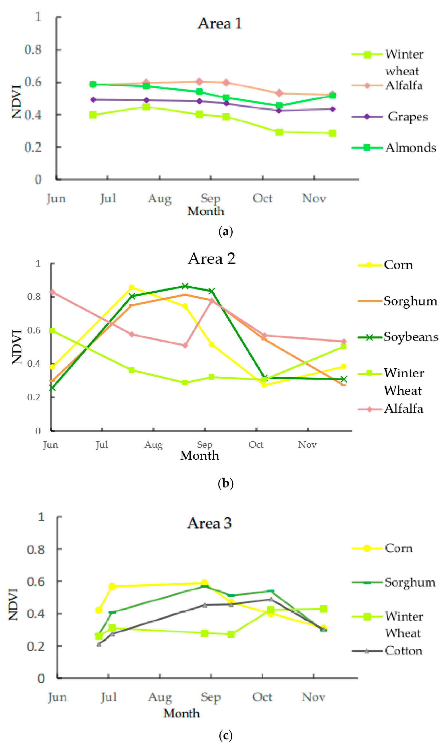
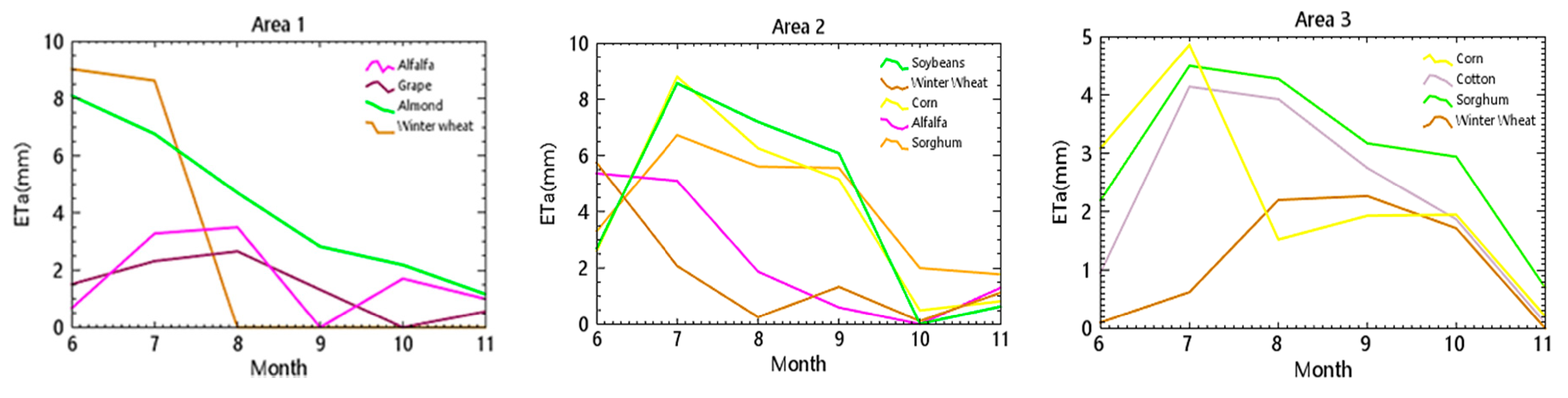
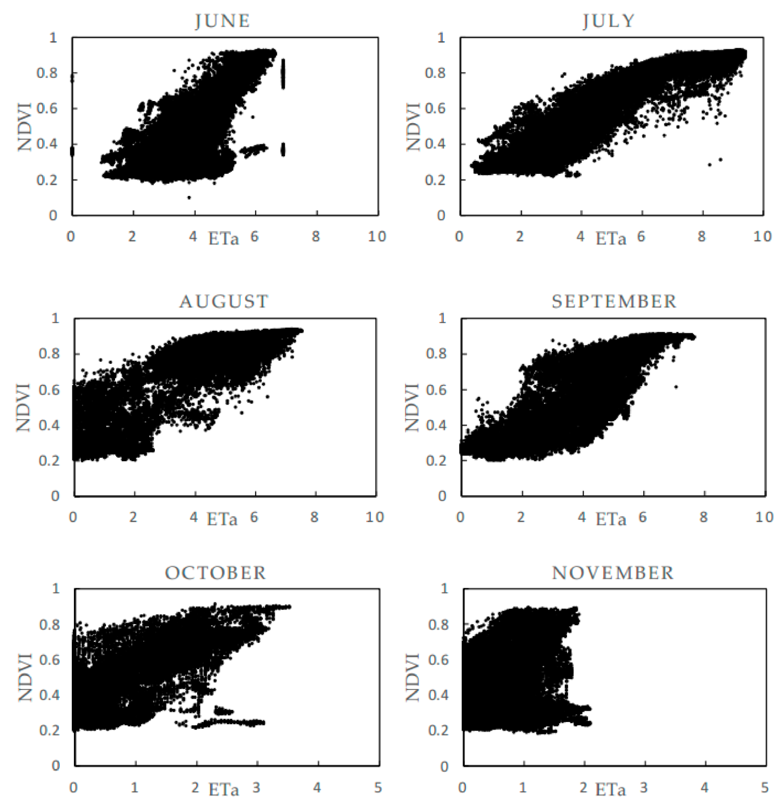
3.1. NDVI and mLSTI of Each Study Area

First, we calculated the average NDVI of the crops, and the NDVI curves of the crops from June to November are shown in Figure 3. There is a clear distinction between winter wheat and other crops in Figure 3a. However, grapes and almonds have a similar growing season. In Figure 3b, there is a clear distinction between corn, alfalfa, and winter wheat; however, the growing season for sorghum and soybeans is similar, which adds to the difficulty in distinguishing sorghum and soybeans. In Figure 3c, there is a similar trend in the NDVI curve changes for sorghum and cotton.

The LST curves and mLSTI curves of the three study areas are shown in Figure 4. The temperature differences between the crops are more evident in the mLSTI curves than in the LST curves. For crops with similar NDVI time series curves in Figure 2, the mLSTI curves show more differences. For example, there are evident differences in the mLSTI curves of grapes and almonds in Figure 3a, sorghum and soybeans in Figure 3b, and sorghum and cotton in Figure 3c.

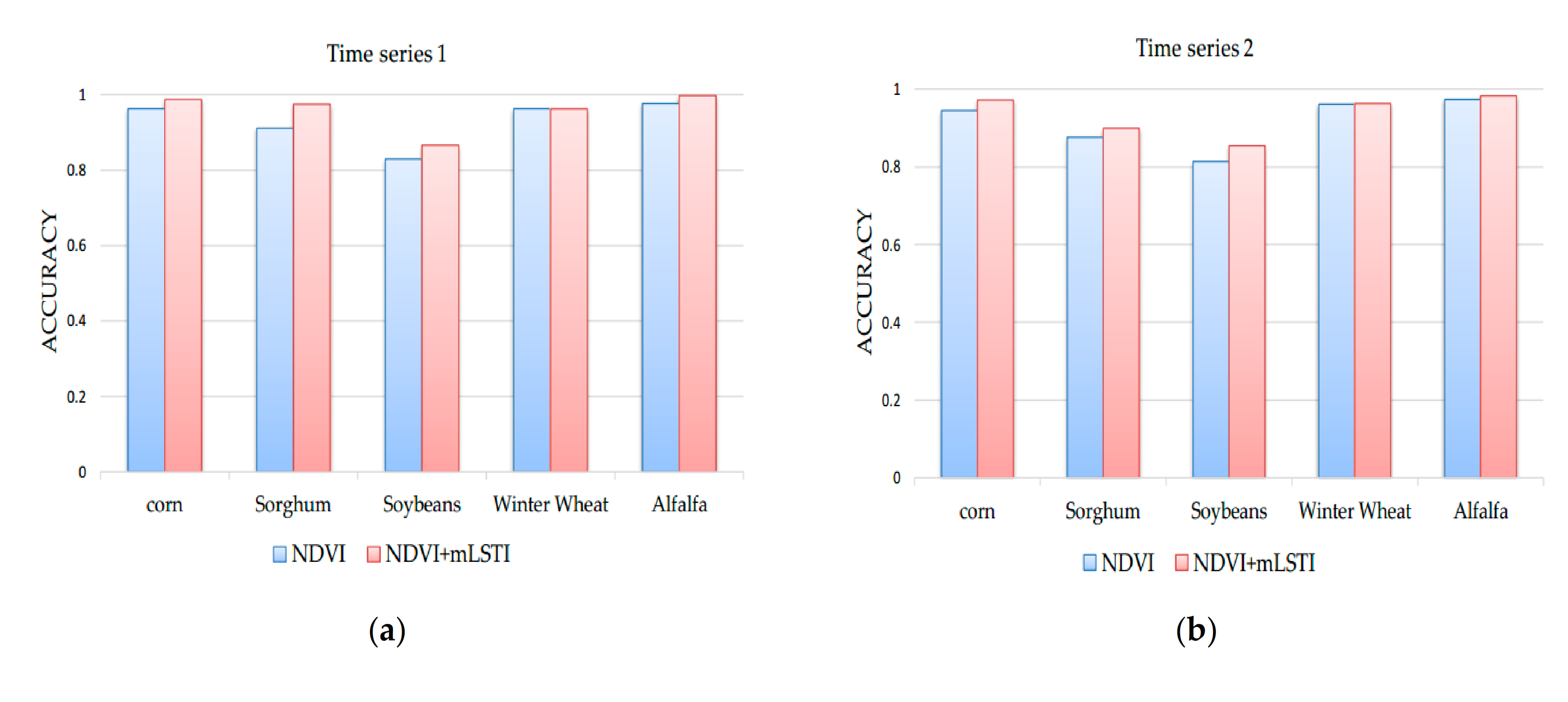
3.2. Classification Results Based on NDVI + mLSTI Long Time Series

Figure 5 shows the results of the crop classification map based on the NDVI + mLSTI long time series from June to November.

The overall classification accuracies for the study areas are listed in

Table 4. Classification accuracy based on the NDVI + mLSTI long time series.

	OA. (%) (NDVI)	OA. (%) (NDVI + mLSTI)
Study area 1	82.0	85.6
Study area 2	94.7	96.3
Study area 3	90.9	91.2

. The high classification accuracy can be attributed to the combined use of the mLSTI and NDVI data.

3.3. Classification Results Based on Short Time Series Feature

The classification accuracies for the four short time series listed in Table 3 are listed in

Table 5. Classification accuracy using different short time series.

	OA. (%) (NDVI) Area 1	OA. (%) (NDVI + mLSTI) Area 1	OA. (%) (NDVI) Area 2	OA. (%) (NDVI + mLSTI) Area 2	OA. (%) (vNDVI) Area 3	OA. (%) (NDVI + mLSTI) Area 3
Times Series 1	80.7	82.7	93.6	96.2	89.4	88.9
Times Series 2	82.1	82.3	92.4	94.0	87.9	87.0
Times Series 3	70.6	81.9	85.5	90.1	86.1	87.4
Times Series 4	66.8	77.5	75.3	80.0	64.7	69.7

. For the different time series, adding the mLSTI time series to the classification process improved the accuracy in most of the cases.

4. Discussion

4.1. Effect of Adding mLSTI on Classification Accuracy

When using long time series from June to November, the overall classification accuracy after adding the mLSTI increased by 3.6% for area 1, 1.6% for area 2, and 0.3% for area 3. For the four shorter time series, after adding the mLSTI time series, the classification accuracy improved in most of the cases, as shown in Figure 6.

For areas 1 and 2, the classification accuracy based on the four short time series improved after adding mLSTI. For area 3, in the case of time series 3 and 4, the accuracy improved significantly, and the accuracy in the case of time series of 1 and 2 decreased slightly. We will analyze this later in this study. The classification accuracy decreased with a decrease in the time length used for the classification, as listed in Table 5. However, compared with the NDVI + mLSTI, the classification accuracy reaches a higher value earlier than using the NDVI. For example, for area 1, when the temporal length of the used data is three months, the classification accuracy is above 80% based on NDVI + mLSTI. However, to reach the same level of accuracy based on NDVI, data from four months is required. For area 2, when the temporal length of the used data is more than three months, the classification accuracy reaches 90% when using the NDVI. However, in the case of three months, the classification accuracy is above 90% when using NDVI + mLSTI. With the addition of the mLSTI time series, shorter time series can be used to achieve a higher classification accuracy, and adding the mLSTI time series is beneficial for timely crop classification.

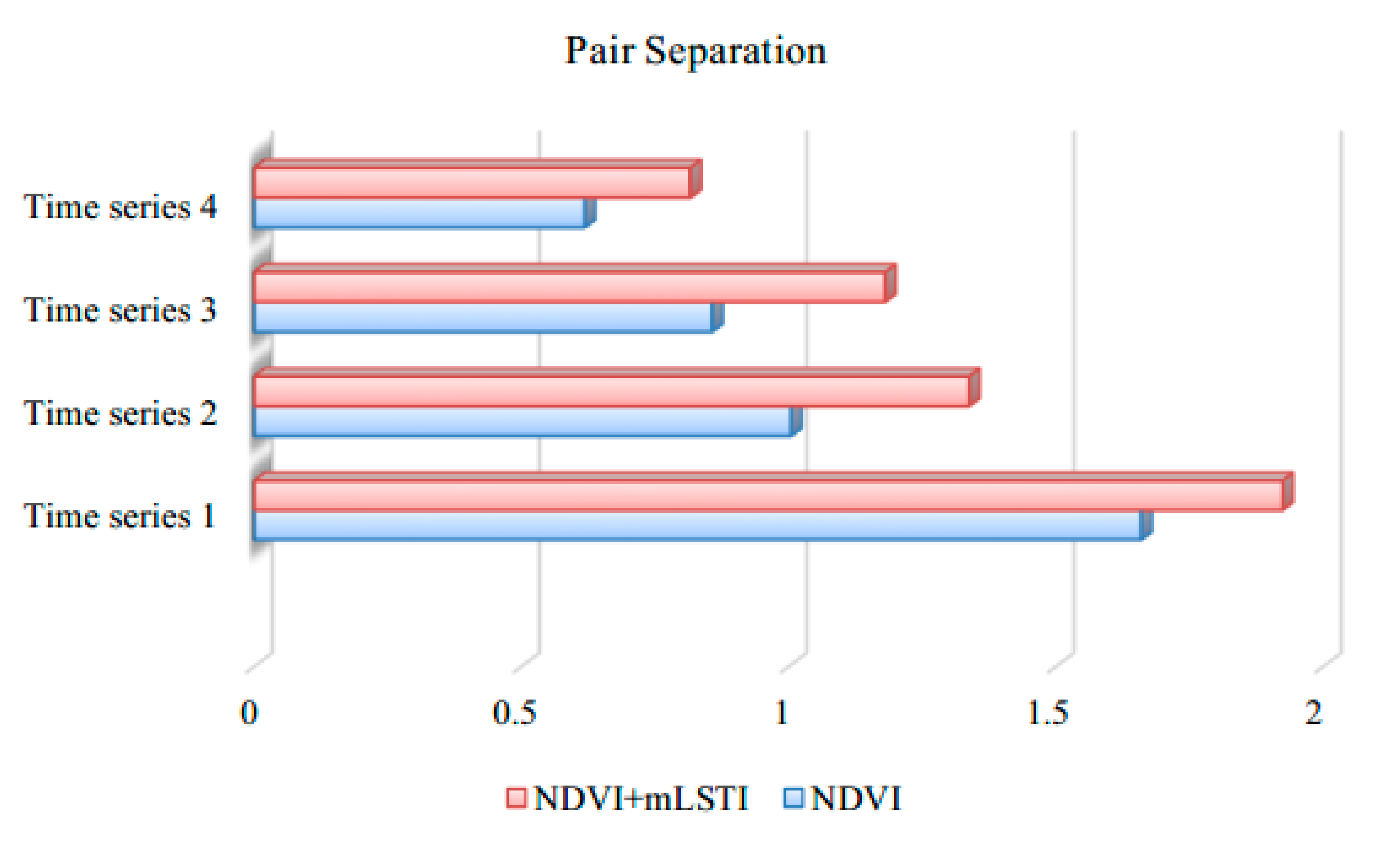
4.2. Effect of Adding mLSTI Time Series on Differentiating Crops

Here, we take study area 2, which has more types of crops, as an example for analysis. For the five crop classes, the classification accuracy is highest when using the NDVI + mLSTI long time series, as shown in

Table 6. Classification accuracies of different crops based on long time series.

	Corn	Sorghum	Soybeans	Winter Wheat	Alfalfa
Prod. Acc. (NDVI) (%)	94.68	92.07	92.94	98.25	91.62
Prod. Acc. (NDVI + mLSTI) (%)	95.89	96.03	96.81	98.55	91.77
User Acc. (NDVI) (%)	95.82	95.32	82.75	96.27	98.71
User Acc. (NDVI + mLSTI) (%)	98.64	97.16	87.90	96.50	98.96

. This demonstrates that the mLSTI time series can help improve the accuracy of differentiating the crops.

For the differentiation of crops using shorter times series, the effects of adding the mLSTI time series to the classification of each crop were compared, as shown in Figure 7. The classification accuracy of various crops after adding the mLSTI is significantly improved. However, we note that there are different degrees of improvement in the classification of the different crops. The classification accuracy of winter wheat is not improved much, as shown in Figure 7. Since the NDVI curve of the winter wheat is quite different from those of the other four crops, the classification accuracy is consistently high for this crop. Therefore, the addition of the mLSTI has little effect on its classification accuracy. The improvements in the classification accuracy of corn, sorghum, and soybeans are more significant. As shown in Figure 3b, the NDVI curves of sorghum and soybeans are similar, since they are both sown in the study area in mid-May. This similarity makes it difficult to distinguish these crops. Nevertheless, the differences in the mLSTI curves can help differentiate soybeans and sorghum.

To further investigate the differentiation of sorghum and soybeans, we studied the separation of sorghum and soybeans using four short time series. We used the Jeffries–Matusita (JM) distance to measure the separability of the crops. The JM distance ranges from 0 to 2, with a higher value indicating a high level of separability [44]. From the results shown in Figure 8, the separation of sorghum and soybeans is significantly improved by 0.13 for time series 1, 0.26 for time series 2, 0.33 for time series 3, and 0.32 for time series 4 after adding the mLSTI time series. The results demonstrate that the NDVI + mLSTI time series has better discrimination ability than NDVI for sorghum and soybeans.

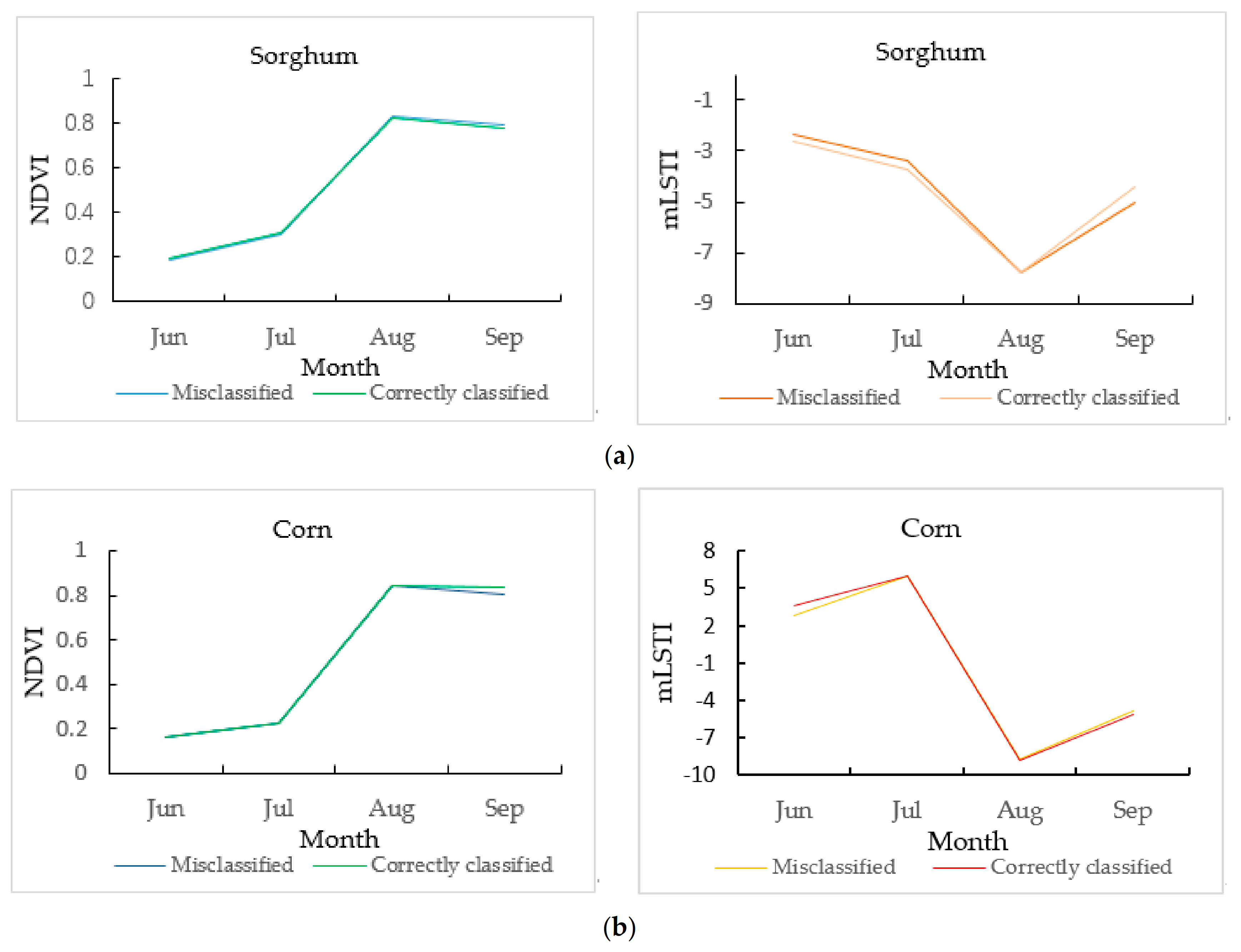
4.3. Analysis of the Reasons for Varying Accuracy after Adding mLSTI

In the samples of the three study areas, we selected an area that includes all of the crop types, and the crops in the selected areas were adjacent to each other. Subsequently, we plotted the mean curves of the ETa for each crop (Figure 9). There are evident differences in the ETa curves of the different crops depicted in Figure 9.

We took study area 2, which has more types of crops, as an example for the analysis. We studied the relationship between mLSTI, ETa, and NDVI for each month. Figure 10 shows the scatter plots of the ETa and mLSTI. The results indicate a good agreement between the ETa and the mLSTI.

Then we studied the scatter plots of the ETa and NDVI for each month (Figure 11). Unlike the clear correlation between the mLSTI and the ETa scatter plots, the NDVI and ETa have no such obvious regular distribution. As mentioned in the introduction, different plant types have different evapotranspiration. The mLSTI and ETa show good correlation (determination coefficient 0.86 for June, 0.99 for July, 0.97 for August, 0.98 for September, 0.80 for October and 0.87 for November), as can be seen in Figure 10, implying that they can reflect the difference in ETa in long time series. However, the relationship between ETa and NDVI is different for different months (the determination coefficient is 0.48 for June, 0.87 for July, 0.85 for August, 0.78 for September, 0.58 for October and 0.04 for November), as shown in Figure 11, so, the NDVI cannot reflect the changing trend of ETa in long time series. Therefore, the addition of mLSTI provides information that cannot be provided by the NDVI.

Figure 6 shows that adding the mLSTI feature to study area 3 is helpful for improving the accuracy in the case of time series 3 (June to August). However, for time series 2 (June to September), the classification accuracy is slightly reduced. Therefore, we focused on the classification difference based on the NDVI and NDVI + mLSTI time series 2.

Table 7. Confusion matrix of study area 3 based on NDVI time series 3.

	Corn	Sorghum	Soybeans	Winter Wheat
Corn (%)	84.3	2.38	18.79	1.17
Sorghum (%)	2.22	92.82	20.44	2.60
Soybeans (%)	13.49	0.60	54.84	1.23
Winter Wheat (%)	0.00	4.20	5.93	94.99

and

Table 8. Confusion matrix of study area 3 based on NDVI + mLSTI time series 3.

	Corn	Sorghum	Soybeans	Winter Wheat
Corn (%)	80.08	1.95	25.27	1.01
Sorghum (%)	2.85	92.86	17.14	2.46
Soybeans (%)	17.05	1.44	51.92	0.52
Winter Wheat (%)	0.03	3.76	5.66	96.01

show the confusion matrix in these two cases. The classification accuracy of corn and sorghum is declining. After adding the mLSTI, corn was more mistakenly classified as sorghum, and sorghum was more mistakenly classified as corn. By examining the misclassified corn and sorghum, we find that the misclassification occurred for areas where the two crops were mixed together. For example, we selected an area where the samples were correctly classified based on the NDVI but misclassified based on the NDVI + mLSTI. We then compare the curves of the misclassified samples and the correctly classified samples in Figure 12. For sorghum, the NDVI curves are very similar; however, there is a significant difference in the mLSTI in September, leading to a misclassification. For corn, although the mLSTI curves are very similar, there is a significant difference in the NDVI in September, leading to a misclassification. The decrease in the accuracy is related to the small planting area and high mixing of the crops. In the above case, it is difficult to use the temperature characteristics to improve the classification.

5. Conclusions

We developed a new approach wherein NDVI and mLSTI time series were combined for the classification of crops in three different areas. The classification accuracy was improved by incorporating the mLSTI time series for most of the classifications.

We analyzed the effect of mLSTI on improving the classification accuracy. First, when using the long time series from June to November, the overall accuracy increased for the three study areas. For the long time series, adding the mLSTI index helped improve the accuracy of crop classification in this study. Second, the proposed approach gave better results compared to those obtained when using only the NDVI for short time series, in most of the cases. Adding the mLSTI feature was found to be beneficial for the timely crop mapping in study areas 1 and 2. For study area 3, when using the short time series, the accuracy was slightly reduced. Through analysis, we found that such a decline occurs in areas where two crops are severely mixed, which indicates that the addition of mLSTI has a limited ability to distinguish severely mixed crops. Third, for differentiating crops that exhibit similar spectro-temporal features, such as soybeans and sorghum in this study, adding the mLSTI time series to the classification provided better discrimination results between such crops. The temperature difference can be used as an auxiliary feature for the differentiation of crops with similar spectro-temporal features in the future.

This study is a first step in using the temperature index for crop classification, and the results suggested the possibility of using thermal information for crop classification. However, this method might be affected by the environment conditions. In the future work, we will focus on the applicability of this method in different climate regions and more follow-up studies should be conducted to supplement the findings.

References

1. Siachalou, S.; Mallinis, G.; Tsakiri-Strati, M. A hidden markov models approach for crop classification: Linking crop phenology to time series of multi-sensor remote sensing data. Remote Sens. 2015, 7, 3633–3650. [Google Scholar] [CrossRef] [Green Version]
2. Murthy, C.S.; Raju, P.V.; Badrinath, K.V.S. Classification of wheat crop with multi-temporal images: Performance of maximum likelihood and artificial neural networks. Int. J. Remote Sens. 2003, 24, 4871–4890. [Google Scholar] [CrossRef]
3. Turker, M.; Arikan, M. Sequential masking classification of multi-temporal Landsat7 ETM+ images for field-based crop mapping in Karacabey, Turkey. Int. J. Remote Sens. 2005, 26, 3813–3830. [Google Scholar] [CrossRef]
4. Ozdogan, M.; Gutman, G. A new methodology to map irrigated areas using multi-temporal MODIS and ancillary data: An application example in the continental US. Remote Sens. Environ. 2008, 112, 3520–3537. [Google Scholar] [CrossRef] [Green Version]
5. Kussul, N.; Lemoine, G.; Gallego, J.; Skakun, S.; Lavreniuk, M. Parcel based classification for agricultural mapping and monitoring using multi-temporal satellite image sequences. In Proceedings of the International Geoscience and Remote Sensing Symposium 2015 (IGARSS 2015), Milan, Italy, 26–31 July 2015; IEEE: New York, NY, USA, 2015. [Google Scholar]
6. Hao, P.; Niu, Z.; Wang, L. Crop classification using multi-temporal HJ satellite images: Case study in Kashgar, Xinjiang. In Proceedings of the Land Surface Remote Sensing II, Beijing, China, 13–16 October 2014; International Society for Optical Engineering: Bellingham, WA, USA, 2014; Volume 9260, p. 926005. [Google Scholar] [CrossRef]
7. Vieira, C.; Mather, P.; McCullagh, M. The spectral-temporal response surface and its use in the multi-sensor, multi- temporal classification of agricultural crops. Int. Arch. Photogramm. Remote Sens. Spat. Inf. Sci. ISPRS Arch. 2000, 33, 582–589. [Google Scholar]
8. Zhang, M.; Li, Q.; Wu, B. Investigating the capability of multi-temporal Landsat images for crop identification in high farmland fragmentation regions. In Proceedings of the International Conference on Agro-Geoinformatics, Shanghai, China, 2–4 August 2012; IEEE: New York, NY, USA; pp. 1–4. [Google Scholar] [CrossRef]
9. Kussul, N.; Skakun, S.; Shelestov, A.; Lavreniuk, M.; Yailymov, B.; Kussul, O. Regional scale crop mapping using multi-temporal satellite imagery. Int. Arch. Photogramm. Remote Sens. Spat. Inf. Sci. ISPRS Arch. 2015, 40, 45–52. [Google Scholar] [CrossRef] [Green Version]
10. Celik, Y.B.; Sertel, E.; Ustundag, B.B. Identification of corn and cotton fields using multi-temporal Spot6 NDVI data. In Proceedings of the 2015 Fourth International Conference on Agro-Geoinformatics, Istanbul, Turkey, 20–24 July 2015; IEEE: New York, NY, USA; pp. 23–26. [Google Scholar]
11. Jakubauskas, M.E.; Legates, D.R.; Kastens, J.H. Crop identification using harmonic analysis of time-series AVHRR NDVI data. Comput. Electron. Agric. 2003, 37, 127–139. [Google Scholar] [CrossRef]
12. Wardlow, B.D.; Egbert, S.L.; Kastens, J.H. Analysis of time-series MODIS 250 m vegetation index data for crop classification in the U.S. Central Great Plains. Remote Sens. Environ. 2007, 108, 290–310. [Google Scholar] [CrossRef] [Green Version]
13. Simonneaux, V.; Duchemin, B.; Helson, D.; Er-Raki, S.; Olioso, A.; Chehbouni, A.G. The use of high-resolution image time series for crop classification and evapotranspiration estimate over an irrigated area in central Morocco. Int. J. Remote Sens. 2008, 29, 95–116. [Google Scholar] [CrossRef] [Green Version]
14. Vintrou, E.; Desbrosse, A.; Bégué, A.; Traoré, S.; Baron, C.; Lo Seen, D. Crop area mapping in West Africa using landscape stratification of MODIS time series and comparison with existing global land products. Int. J. Appl. Earth Obs. Geoinf. 2012, 14, 83–93. [Google Scholar] [CrossRef]
15. Xinchuan, L.; Xingang, X.; Jihua, W.; Hongfeng, W.; Yansong, B. Crop classification recognition based on time-series images from hj satellite. Nongye Gongcheng Xuebao/Trans. Chin. Soc. Agric. Eng. 2013, 29, 2013. [Google Scholar] [CrossRef]
16. Piedelobo, L.; Hernández-López, D.; Ballesteros, R.; Chakhar, A.; Del Pozo, S.; González-Aguilera, D.; Moreno, M.A. Scalable pixel-based crop classification combining Sentinel-2 and Landsat-8 data time series: Case study of the Duero river basin. Agric. Syst. 2019, 171, 36–50. [Google Scholar] [CrossRef]
17. Conrad, C.; Colditz, R.R.; Dech, S.; Klein, D.; Vlek, P.L.G. Temporal segmentation of MODIS time series for improving crop classification in Central Asian irrigation systems. Int. J. Remote Sens. 2011, 32, 8763–8778. [Google Scholar] [CrossRef]
18. Hao, P.; Tang, H.; Chen, Z.; Liu, Z. Early-season crop mapping using improved artificial immune network (IAIN) and Sentinel data. PeerJ 2018, 1–30. [Google Scholar] [CrossRef]
19. De Souza, C.H.W.; Mercante, E.; Johann, J.A.; Lamparelli, R.A.C.; Uribe-Opazo, M.A. Mapping and discrimination of soya bean and corn crops using spectro-temporal profiles of vegetation indices. Int. J. Remote Sens. 2015, 36, 1809–1824. [Google Scholar] [CrossRef]
20. Stan, F.I.; Neculau, G.; Zaharia, L.; Ioana-Toroimac, G. Evapotranspiration variability of different plant types at romanian experimental evapometric measurement stations. Climatologie 2014, 11, 1962–1966. [Google Scholar] [CrossRef]
21. Al-Kaisi, M.M.; Broner, I. Crop water use and growth stages. Colo. State Univ. Ext. 2009, 4, 4–9. [Google Scholar]
22. DeJonge, K.C.; Taghvaeian, S.; Trout, T.J.; Comas, L.H. Comparison of canopy temperature-based water stress indices for maize. Agric. Water Manag. 2015, 156, 51–62. [Google Scholar] [CrossRef]
23. Siebert, S.; Webber, H.; Zhao, G.; Ewert, F. Heat stress is overestimated in climate impact studies for irrigated agriculture. Environ. Res. Lett. 2017, 12. [Google Scholar] [CrossRef]
24. Meier, F.; Scherer, D. Spatial and temporal variability of urban tree canopy temperature during summer 2010 in Berlin, Germany. Theor. Appl. Climatol. 2012, 110, 373–384. [Google Scholar] [CrossRef]
25. Blum, M.; Lensky, I.M.; Nestel, D. Estimation of olive grove canopy temperature from MODIS thermal imagery is more accurate than interpolation from meteorological stations. Agric. For. Meteorol. 2013, 176, 90–93. [Google Scholar] [CrossRef]
26. NASS, USDA. 2017 California Cropland Data Layer; USDA, NASS Marketing and Information Services Office: Washington, DC, USA, 2017. Available online: https://nassgeodata.gmu.edu/CropScape/ (accessed on 26 January 2018).
27. NASS, USDA. 2016 Kansas Cropland Data Layer; USDA, NASS Marketing and Information Services Office: Washington, DC, USA, 2016. Available online: https://nassgeodata.gmu.edu/CropScape/ (accessed on 30 January 2017).
28. NASS, USDA. 2019 Texas Cropland Data Layer; USDA, NASS Marketing and Information Services Office: Washington, DC, USA, 2019. Available online: https://nassgeodata.gmu.edu/CropScape/ (accessed on 3 February 2020).
29. Vermote, E.; Justice, C.; Claverie, M.; Franch, B. Preliminary analysis of the performance of the Landsat 8/OLI land surface reflectance product. Remote Sens. Environ. 2016, 185, 46–56. [Google Scholar] [CrossRef] [PubMed]
30. Cook, M.J.; Schott, J.R. Initial validation of atmospheric compensation for a Landsat land surface temperature product. In Algorithms and Technologies for Multispectral, Hyperspectral, and Ultraspectral Imagery XIX; International Society for Optics and Photonics: Bellingham, WA, USA, 2013; Volume 8743, p. 874314. [Google Scholar] [CrossRef]
31. Cook, M.; Schott, J.R.; Mandel, J.; Raqueno, N. Development of an operational calibration methodology for the Landsat thermal data archive and initial testing of the atmospheric compensation component of a land surface temperature (LST) product from the archive. Remote Sens. 2014, 6, 11244–11266. [Google Scholar] [CrossRef] [Green Version]
32. Howard, D.M.; Wylie, B.K.; Tieszen, L.L. Crop classification modelling using remote sensing and environmental data in the Greater Platte River Basin, USA. Int. J. Remote Sens. 2012, 33, 6094–6108. [Google Scholar] [CrossRef]
33. Li, Q.; Wang, C.; Zhang, B.; Lu, L. Object-based crop classification with Landsat-MODIS enhanced time-series data. Remote Sens. 2015, 7, 16091–16107. [Google Scholar] [CrossRef] [Green Version]
34. Hao, P.; Zhan, Y.; Wang, L.; Niu, Z.; Shakir, M. Feature selection of time series MODIS data for early crop classification using random forest: A case study in Kansas, USA. Remote Sens. 2015, 7, 5347–5369. [Google Scholar] [CrossRef] [Green Version]
35. Momm, H.G.; ElKadiri, R.; Porter, W. Crop-type classification for long-term modeling: An integrated remote sensing and machine learning approach. Remote Sens. 2020, 12, 449. [Google Scholar] [CrossRef] [Green Version]
36. Boryan, C.G.; Yang, Z.; Willis, P. US geospatial crop frequency data layers. In Proceedings of the Third International Conference on Agro-geoinformatics, Beijing, China, 11–14 August 2014; IEEE: New York, NY, USA. [Google Scholar] [CrossRef]
37. Ji, S.; Zhang, C.; Xu, A.; Shi, Y.; Duan, Y. 3D convolutional neural networks for crop classification with multi-temporal remote sensing images. Remote Sens. 2018, 10, 75. [Google Scholar] [CrossRef] [Green Version]
38. Rodriguez-Galiano, V.F.; Ghimire, B.; Rogan, J.; Chica-Olmo, M.; Rigol-Sanchez, J.P. An assessment of the effectiveness of a random forest classifier for land-cover classification. ISPRS J. Photogramm. Remote Sens. 2012, 67, 93–104. [Google Scholar] [CrossRef]
39. Liu, J.; Feng, Q.; Gong, J.; Zhou, J.; Liang, J.; Li, Y. Winter wheat mapping using a random forest classifier combined with multi-temporal and multi-sensor data. Int. J. Digit. Earth 2018, 11, 783–802. [Google Scholar] [CrossRef]
40. Breiman, L. ST4_Method_Random_Forest. Mach. Learn. 2001, 45, 5–32. [Google Scholar] [CrossRef] [Green Version]
41. Cutler, A.; Cutler, D.R.; Stevens, J.R. Random forests. Ensemble Mach. Learn. 2012. [Google Scholar] [CrossRef]
42. Jhonnerie, R.; Siregar, V.P.; Nababan, B.; Prasetyo, L.B.; Wouthuyzen, S. Random Forest Classification for Mangrove Land Cover Mapping Using Landsat 5 TM and ALOS PALSAR Imageries. Procedia Environ. Sci. 2015, 24, 215–221. [Google Scholar] [CrossRef] [Green Version]
43. Hay, A.M. Remote sensing letters the derivation of global estimates from a confusion matrix. Int. J. Remote Sens. 1988, 9, 1395–1398. [Google Scholar] [CrossRef]
44. Bruzzone, L.; Roli, F.; Serpico, S.B. An Extension of the Jeffreys-Matusita Distance to Multiclass Cases for Feature Selection. IEEE Trans. Geosci. Remote Sens. 1995, 33, 1318–1321. [Google Scholar] [CrossRef] [Green Version]
Figure 1. Location of the study sites: (a) Landsat 8 image of study area 1 in California taken on 25 July 2017, (b) Landsat 8 image of study area 2 in Kansas taken on 20 July 2016, and (c) Landsat 8 image of study area 3 in Texas taken on 4 July 2019.
Remotesensing 12 03202 g001
Figure 2. Flowchart of the research process.
Remotesensing 12 03202 g002
Figure 3. The normalized difference vegetation index (NDVI) curves of crops grown in (a) study area 1, (b) study area 2, and (c) study area 3.
Remotesensing 12 03202 g003
Figure 4. The land surface temperature (LST) and the modified land surface temperature index (mLSTI) curves of (a) study area 1, (b) study area 2, and (c) study area 3.
Remotesensing 12 03202 g004
Figure 5. Crop classification maps obtained using NDVI + mLSTI long time series of: (a) study area 1, (b) study area 2, and (c) study area 3.
Remotesensing 12 03202 g005
Figure 6. Improved classification accuracy in the study areas after adding mLSTI.
Remotesensing 12 03202 g006
Figure 7. Comparison of the classification accuracies of crops based on short time series: (a) time series 1, (b) time series 2, (c) time series 3, and (d) time series 4.
Remotesensing 12 03202 g007aRemotesensing 12 03202 g007b
Figure 8. Separation of sorghum and soybeans.
Remotesensing 12 03202 g008
Figure 9. Mean curves of the actual evapotranspiration (ETa) for each crop.
Remotesensing 12 03202 g009
Figure 10. Scatter plots of ETa and mLSTI.
Remotesensing 12 03202 g010
Figure 11. Scatter plots of ETa and NDVI.
Remotesensing 12 03202 g011
Figure 12. Mean NDVI and mLSTI curves of the selected area in area 2 for (a) sorghum, and (b) corn.
Remotesensing 12 03202 g012