Article

sUAS Remote Sensing of Vineyard Evapotranspiration Quantifies Spatiotemporal Uncertainty in Satellite-Borne ET Estimates

by
Michael Kalua
1,2,
Anna M. Rallings
1,2,
Lorenzo Booth
1,3,
Josué Medellín-Azuara
1,2,
Stefano Carpin
1,3 and
Joshua H. Viers
1,2,*
1
Center for Information Technology Research in the Interest of Society and the Banatao Institute, University of California, Merced, CA 95343, USA
2
Civil & Environmental Engineering, University of California, Merced, CA 95343, USA
3
Computer Science Engineering, University of California, Merced, CA 95343, USA
*
Author to whom correspondence should be addressed.
Remote Sens. 2020, 12(19), 3251; https://doi.org/10.3390/rs12193251
Submission received: 21 August 2020 / Revised: 24 September 2020 / Accepted: 25 September 2020 / Published: 7 October 2020
(This article belongs to the Special Issue Remote Sensing in Hydrology and Water Resources Management)

Abstract

:
Small Unmanned Aerial Systems (sUAS) show promise in being able to collect high resolution spatiotemporal data over small extents. Use of such remote sensing platforms also show promise for quantifying uncertainty in more ubiquitous Earth Observation System (EOS) data, such as evapotranspiration and consumptive use of water in agricultural systems. This study compares measurements of evapotranspiration (ET) from a commercial vineyard in California using data collected from sUAS and EOS sources for 10 events over a growing season using multiple ET estimation methods. Results indicate that sUAS ET estimates that include non-canopy pixels are generally lower on average than EOS methods by >0.5 mm day 1 . sUAS ET estimates that mask out non-canopy pixels are generally higher than EOS methods by <0.5 mm day 1 . Masked sUAS ET estimates are less variable than unmasked sUAS and EOS ET estimates. This study indicates that limited deployment of sUAS can provide important estimates of uncertainty in EOS ET estimations for larger areas and to also improve irrigation management at a local scale.

Graphical Abstract

1. Introduction

Global environmental change and anthropogenic activity have long stressed Earth’s hydrological cycle [1,2]. Evapotranspiration remains the least certain quantified component of the hydrological cycle [3], with implications for not only water resources planning and management, but also for human livelihoods and supporting ecosystems [4]. Globally, irrigated agriculture represents 70% of water withdrawn from surface and ground water supplies but estimates of actual consumptive loss (the largest component of the water balance in an agricultural region) through evapotranspiration (ET) remain coarse [5]. New advances in satellite remote sensing of ET via Earth Observation Systems (EOS) show promise in providing consistent and reliable quantitative estimates with global coverage and reasonable repeat cycles. However, the spatiotemporal resolution of EOS platforms and sensors may obscure finer spatial resolution phenomena or weather-related aberrations observed at finer time scales. Small Unmanned Aerial Systems (sUAS) operated under the Federal Aviation Administration (FAA) Part 107 licensing outfitted with optical sensors are increasingly used in vegetation remote sensing [6] and precision agriculture applications [7]. More recently, however, comparative studies of EOS and sUAS observations of crop water stress have shown significant spatiotemporal uncertainty in coarser EOS data [8,9].

1.1. Evapotranspiration in Water Management

Globally, freshwater withdrawals have increased five-fold over the past century [10]. While rain-fed agriculture is most widespread, representing approximately 78% of water use in agriculture, irrigated agriculture is most prevalent in arid and semi-arid parts of the globe, such as the Mediterranean biome that is characterized by cool, wet winters and dry, hot summers [11]. This region, extending beyond the Mediterranean basin to include portions of Australia, Chile, South Africa, and California (USA) is also characterized by expansive urbanization and high intensity agriculture [11]. The productivity of agriculture in such places, especially in California, is achieved in part because of the ideal growing conditions, resulting in hundreds of different agricultural commodities, but also because of expansive water development infrastructure built primarily to meet irrigation demand [12]. California is the most agriculturally productive region in the USA [13], but also one of the world’s most water stressed [14,15]. Like much of the Mediterranean biome, California is characterized by pronounced wet and dry periods, both intra- and inter-annually. More recently, however, extreme variation in precipitation has resulted in exceptionally wet events and prolonged dry droughts [16,17]. Managing California’s water has thus become more challenging [18], and therefore a better understanding agricultural consumptive water use (i.e., ET) is a critical need.
In a recent comprehensive study by Medellín-Azuara et al. [19], seven different ET calculation methods involving remotely sensed data, satellite imagery and ground level meteorological stations were evaluated for their performance in quantifying ET for the heavily cultivated Sacramento-San Joaquin Delta region of California over a period of two growing seasons (2015–2016). While there was general consensus between these seven methods, model results were only within 20% of the median estimate for total consumptive use. This high level of uncertainty has implications not only for broad water resources management decisions across California, but also limits local decision-making by individual growers if they are unable to know how much water is needed when and where. Improving reliability of coarse ET estimates, therefore, would improve water management decision-making more broadly by balancing demand with supply [20] and also could accelerate adoption of irrigation methods that leverage real-time information on crop water demand [21]. When coupled with localized monitoring, such as with sUAS remote sensing of evapotranspiration, these technologies have the potential to integrate other ecologically-friendly practices [22].

1.2. Remote Sensing of Evapotranspiration

Evapotranspiration has long been the focus of hydrological and agrometeorological studies [23,24]. Zhang et al. [25] reviewed the state of science in remote sensing of evapotranspiration (RSE), described its use to estimate and map ET at regional to continental scales, and highlighted existing major RSE estimation methods. Because so many studies and reviews have been conducted on ET measurements, modeling and RSE methods of retrieval, they are not repeated here. Rather, we focus on the fact that RSE from EOS provides relatively frequent, consistent, and spatially contiguous measurements for global estimation, monitoring, and mapping of ET flux; however, due to the relatively coarse granularity of such data at the field level, we explore how high spatiotemporal resolution data from sUAS could quantify inherent variability in such estimates.
In almost all cases, RSE relies on energy balance methods. Most RSE methods focused on energy balance are rooted in Surface Energy Balance Algorithm for Land (SEBAL) [26,27,28] an image-processing model to quantify surface energy balance components, at both local and regional scales using empirical relationships and physical parameterization. SEBAL requires digital imagery data collected by any satellite sensor measuring visible, near-infrared, and thermal infrared radiation, and their derivative products including surface temperature, normalized difference vegetation index (NDVI), and albedo. SEBAL was a methodological precursor to METRIC (Mapping EvapoTranspiration at high Resolution with Internalized Calibration), developed by Allen et al. [29], which is now a standard remote sensing estimation approach using Landsat 5, 7 and 8 EOS imagery (including thermal bands), local weather station data, and calibrated from either nearby alfalfa or pasture, and bare soil land cover types. Landsat-based METRIC, and other similar approaches are described in Irmak et al. [30].
More recently, a number of open-source methods have emerged as Google Earth Engine-based collaborative [31]. One such method includes EEFlux, a version of the METRIC model as developed by Morton et al. [31] employing algorithms by Irmak et al. [30]; EEFlux has been used because of expansive access to EOS imagery and computational assets, including built-in calibration using reference ET from the North America Land Data Assimilation System [32,33] and GridMET [34] for the contiguous United States. In implementation, however, RSE methods such as these are explicitly reliant upon thermal infrared sensors ( λ = 10,500–12,510 nm) onboard EOS platforms, which largely prohibits inclusion of field-deployed sUAS RSE methods of comparison because of the limited performance and calibration difficulty experienced by small thermal infrared sensors [35,36]. Full-scale incorporation of sUAS thermal-based RSE remains elusive to most practitioners due to the fact that transmissivity and atmospheric radiance vary dramatically throughout the day [37] and that most sUAS data collection missions can last several hours.
A more direct comparison of RSE between EOS and sUAS approaches, due in part to the prevalence of low-cost commercial multispectral sensors for sUAS, would provide practitioners a means by which to evaluate coarse EOS RSE estimates to finer resolution RSE estimates from local collections. For cross-platform RSE comparison, without inclusion of thermal measurements, it is necessary then to focus on methods that use photosynthetic productivity as a proxy for ET using available spectral response in the 400–900 nm domain (Figure 1). This transfer function approach to RSE is increasingly driven by studies of robust empirical relation between image-derived estimates of vegetation greenness (i.e., NDVI) and ET [38], wherein cellular light energy in red wavelengths is absorbed by chlorophylls and near-infrared light energy is reflected by plant lignin and cellulose. It should be noted here that robust comparisons between EOS data products requires harmonization techniques [39] not employed here. For the purposes of this study, we also explore the utility of OpenET NDVI-ET and SSEBop estimates as described in more detail below.

1.3. Research Questions

Given the importance of ET in water management generally, and the potential uncertainty of EOS ET estimation for large seemingly homogeneous cropping areas with temporal variance, we explored several research questions to help parameterize the spatiotemporal uncertainty of EOS ET estimation using sUAS RSE. Answers to these research questions can provide practitioners valuable qualifiers of uncertainty as EOS ET estimates are now more routinely used in determining irrigation volumes and scheduling. Through cross-platform comparisons, we asked:
  • Do EOS and sUAS ET estimates fundamentally differ over same period of time? In other words, over the course of the growing season, does either the mean or variance of sUAS and EOS ET estimates differ? While we expect that ET estimates to similarly track the growing season (e.g., peak ET demand in mid-summer), it remains unknown if the variance in ET estimates also track either the growing season or each other, sUAS compared to EOS. By using the fixed temporal domain of the growing season and coincident measurements, we can compare upscaled sUAS ET to EOS ET estimates to determine if temporal variance is uniformly distributed or varies across time.
  • Do EOS and sUAS ET estimates fundamentally differ over the same study domain and same period of time? While we expect that the mean ET should be comparable from pixel to pixel, it remains unknown if the variance will differ in either within an EOS pixel or across the pixel domain. By using the fixed spatial domain of the vineyard block and by comparing upscaled sUAS ET to EOS ET estimates within and across pixels, we can retain the spatial variance of sUAS to determine if sUAS spatial variance is greater than EOS pixel to pixel variance.
  • Do “mixed pixels” inherent in EOS data obscure important signals in ET estimation? Over the course of a growing season, biomass and leaf area index can change, altering reflectance and ultimately energy balance models. We evaluated the canopy fraction using high spatial resolution sUAS imagery and vineyard canopy structure to determine if unobscured plant reflectance values were better proxies for ET estimation.

2. Materials and Methods
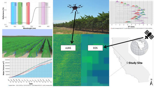
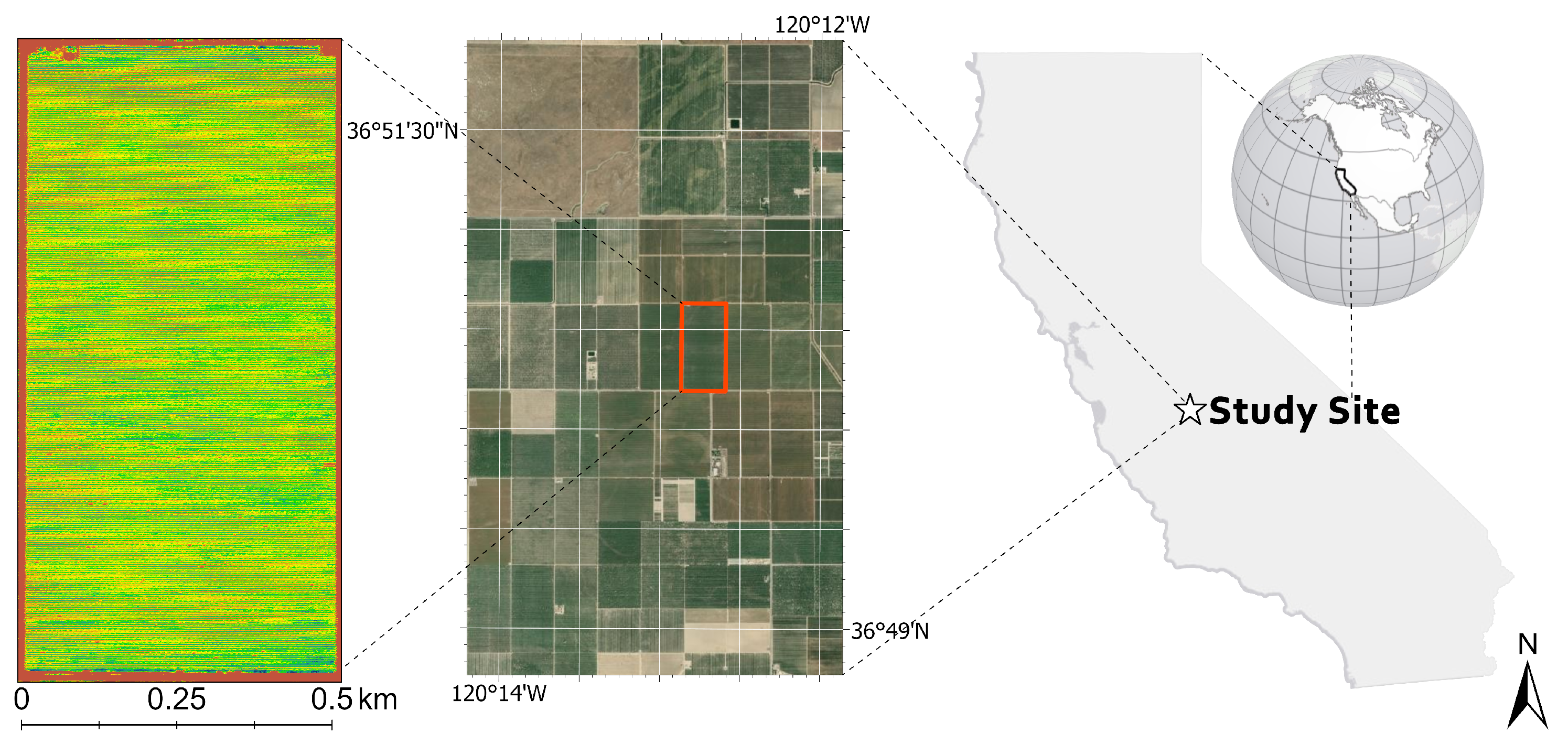
We evaluated cross-platform data products and methods to estimate ET in a high-yield commercial winegrape vineyard. We used small Unmanned Aerial Systems (sUAS) to capture high-spatiotemporal, multispectral imagery to compare to well-established EOS Landsat 8 (https://landsat.gsfc.nasa.gov/landsat-8/) and Sentinel 2 (https://sentinel.esa.int/web/sentinel/missions/sentinel-2) systems. We timed our sUAS field campaigns to coincide with EOS overpasses. We used EOS imagery to calculate ET using both a reflectance based NDVI approach and the emerging EEFlux approach. For EOS ET estimates, Sentinel 2 Bottom of Atmosphere reflectance imagery was used for the OpenET NDVI model and Landsat 8 was used for EEFlux. sUAS imagery was calibrated, stitched, and georeferenced to produce reflectance and structure-from-motion (SfM) surface model products. The OpenET NDVI model approach [31] was used to generate high resolution sUAS-based ET estimates from reflectance, and surface models were used to identify canopy and ground pixels to mask soil in subsequent analysis. As single date LiDAR collection was used to validate SfM canopy models. Each platform’s raster-based ET estimates were resampled to have consistent spatial origin, extent, resolution and index to track coincident pixel value and change throughout the season and across data source. We used a combination of Ardupilot Mission Planner (v.1.3.59), Pix4D Pix4DMapper (v.4.3.3), Phoenix LiDAR Systems SpatialFuser (v.3.5.1) and CloudCompare (v.2.11 alpha) for sUAS data collection and manipulation; ESA Snap Toolbox (v.6.0), OSGeo GDAL (v.2.3.2), Google Earth Engine Python API (v.0.1.217), Python (v.3.6) and ESRI ArcMap (v.10.5.1) for EOS data manipulation; and ESRI ArcGIS Pro (v.2.4) and R (v.3.5.3) for platform comparison and analysis.

2.1. Study Site

The study site was a commercial vineyard located in Ripperdan, Madera County, California, USA (Figure 2; 3650 24.39 N , 12012 43.29 W). The analysis evaluated a 31.23 hectare block, consisting of Chardonnay vines (Vitis vinifera) and planted in 2009 on 1103P rootstock and double vertical canopy trellising. Primary viticultural techniques included use of drip irrigation and annual cover-cropping with oats (45%), barley (45%), and mustard (10%). Site soils consisted of Dinuba-El Peco alkaline fine sandy loam for the majority of the vineyard block, and a Grangeville sandy loam distributed in what appears to be remnant stream bed coursing through the northwest corner. Data were collected on 10 site visits for the period of May–September 2018. Across the growing season, the air temperature ranged 5.2–40.1 °C, minimum to maximum daily measured hourly, and resulted in 2058 degree days. For the calendar year 2018, the site received 733 mm of rainfall. Site observations and agronomic records indicate uniformity of vine canopy growth, and hence soil exposure, for each date of site visitation and across the growing season.

2.2. Analytical Methods

2.2.1. Reference Evapotranspiration

Reference evapotranspiration describes the fraction of ET from a reference crop given measured weather conditions. In the METRIC energy balance method, reference ET (ET ref ) is typically based on the ratio of irrigated alfalfa, the reference crop, to ET o for grass. ET ref was collected from Spatial CIMIS [40], to obtain daily ET o for the study vineyard throughout the growing season. Spatial CIMIS renders ET o at a 2-km spatial resolution by coupling daily solar radiation from NOAA GOES satellite with the Heliosat-II method [41] and interpolating air temperature T, relative humidity RH, and wind speed u 2 from CIMIS stations. ET o is calculated using a modified ASCE–Penman Montieth equation for clipped grass reference from [42] (Equation (1)):
E T o = 0.408 Δ ( R n G ) + γ 900 T + 273 u 2 ( e s e a ) Δ + γ ( 1 + 0.34 u 2 )
where ET o is reference crop evapotranspiration (mm day 1 , R n is net radiation at the crop surface (MJ m 2 day 1 , G is soil heat flux density at the soil surface (MJ m 2 day 1 , T is the daily mean air temperature at 2 m (ms 1 , u 2 is wind speed at 2 m, the difference e s e a is the saturation vapor pressure deficit (kPa), γ is the psychrometric constant ( 66 Pa K 1 , and Δ is the slope of the saturation vapor pressure-temperature curve (kPa °C 1 ).

2.2.2. Earth Engine Flux

Earth Engine Flux (EEFlux) is an implementation of METRIC [29] in Google Earth Engine for Landsat or MODIS imagery with automatic calibration using groundlevel weather station data, land-use data, and a digital elevation model that calculates the residual latent energy used to evaporate water. EEFlux uses GridMET weather data to calculate daily ET ref with the Standardized ASCE-PM equation. EEFlux allows users to select a region of interest, range of dates, and satellite overpasses to calculate ET using the METRIC surface energy balance method in a matter of minutes. We obtained 11 EEFlux Landsat 8 daily ET products from 16 April to 23 September for the 2018 growing season.

2.2.3. OpenET

OpenET (https://etdata.org/) is a collection of Google Earth Engine-based ET models. OpenET is currently in beta with some features accessible on Github, including SSEBop and an NDVI-based ET model. Both NDVI-ET and SSEBop models are run via Google’s Earth Engine Python API (https://github.com/google/earthengine-api). While NDVI can be used as a proxy for photosynthetic activity, it has also been shown to vary linearly with E T o . Daily O p e n E T a N D V I rasters were used to produce a dimensionless ET fraction (ET f ) raster by using a linear model adjusted for E T o . NDVI was calculated using the Red and NIR bands from each platform (see Figure 1 and Equation (2)) (S2: Bands 4 (650–680 nm) and 8 (785–899 nm); sUAS: Red (663–673 nm) and NIR (820–860 nm)). A slope coefficient of 1.25 and intercept of 0 were set to conform to OpenET NDVI-ET-Beta model parameters [31]. Daily ET rasters were created for both models (NDVI-ET and SSEBop) and used for model comparison. EOS imagery was processed through Earth Engine. sUAS imagery was processed in ArcGIS Pro 2.4 following OpenET’s NDVI-ET method.
The linear transfer function for O p e n E T a N D V I is as follows:
O p e n E T a N D V I = 1.25 ( σ NIR σ RED σ NIR + σ RED ) E T o
where σ NIR is reflectance in the near infrared band and σ RED is reflectance in the red band (see Figure 1). E T o was derived from from Spatial CIMIS, such that E T a is actual ET (mm day 1 ) and E T o is daily reference ET from Spatial CIMIS (mm day 1 ).

2.3. Data Products

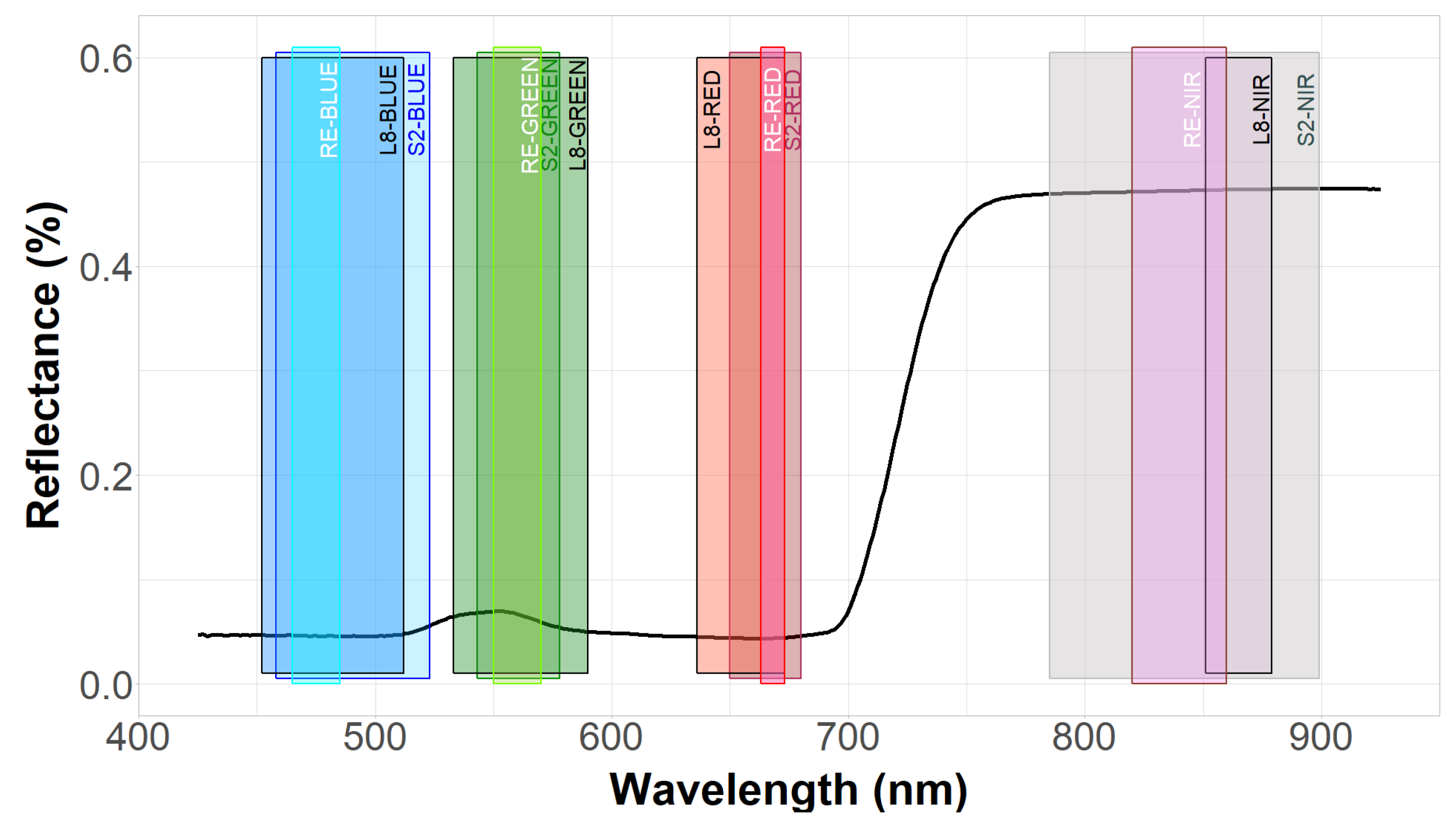
2.3.1. Satellite Imagery

Sentinel 2 imagery was collected from USGS EarthExplorer for each coinciding overpass with a field survey and overpasses within 3 days of a Landsat overpass. Level 1C Top of Atmosphere products were run through the Sen2Cor plugin (ESA, v.2.5.5) in SNAP Toolbox (ESA, v.6.0). Sen2Cor was used to correct for any atmospheric effects and to produce Level 2A Bottom of Atmosphere reflectance products. Corrected Sentinel data were transformed from JPEG2000 to GeoTiff format using GDAL, and subsequently analyzed in ArcGIS and R for cross-platform comparisons. No attempt was made to harmonize Landsat and Sentinel imagery vis-à-vis Claverie et al. [43] given the limited availability of such data to grower practitioners.

2.3.2. sUAS Imagery and Ancillary Data

Data Acquisition Flights: All sUAS missions were planned with Ardupilot Mission Planner to maintain a consistent flight pattern over the 10 acquisition dates between April and September 2018. Each flight was operated under FAA Part 107 flight rules by a certified Remote Pilot. The early season flights in April and May were completed using the Finwing Sabre; a foam fixed-wing sUAS, carrying a Parrot Sequioa sensor. Subsequent flights were flown with a DJI S1000 multirotor sUAS carrying a Micasense Red Edge-M sensor. Multirotor flights (DJI S1000) were flown in a simple grid pattern with transects in a north-south orientation (90 m Altitude, 80% Sidelap, 80% Frontlap, 9 m s 1 speed, 20 m flightline spacing). Most dates required four flights to cover the entire vineyard block at the desired altitude, front and side overlap. Additional flights were performed in case of sensor drop-outs or wind reducing flight endurance. Flights were completed as close to solar noon to minimize shadows.
Canopy Volume: We used a voxel approach to calculate the volume of the canopy for each of the RSE flight over the growing season. Canopy volume was calculated for each flight date with a densified point cloud from Pix4D. The densified point cloud was then classified in CloudCompare using the Cloth Simulation Filter [44]. Once ground and non-ground points were identified, a 25 cm Digital Terrain Model (DTM) was made from using only ground points and a 25 cm Digital Surface Model (DSM) was made from using all points to model the canopy as well as the bare soil elevation. The DTM was subtracted from the DSM to produce a Canopy Height Model (CHM) for each applicable date. The CHM was then multiplied by the area of each cell to calculate the canopy volume of the full field. The CHM was also used to create an above ground canopy mask used to exclude bare soil and cover crop in subsequent analyses.
Reflectance Imagery: Reflectance images from the Parrot Sequoia and Micasense Red Edge-M were georeferenced and stitched through the photogrammetry software Pix4DMapper Pix4D, version 4.3.3, 2018-04-09). RTK GPS-surveyed Ground Control Points (GCPs) were used for each flight to ensure accurate orthomosaic geolocation. Our sUAS ET model used orthomosaics of reflectance values and DSMs produced for each flight date. Model results were upscaled to 10 m spatial resolution to conform with Sentinel 2 pixel geometry. The upscaled outputs included mean, maximum, minimum, and standard deviation of the finer sUAS pixel values within each Sentinel 2 pixel.

3. Results

3.1. Irrigation Delivery and Canopy Growth

Observed irrigation practices for the growing season resulted in a average of 5.26 mm day 1 across the growing season and 9.96 mm day 1 for irrigation days, but varied considerably across the growing season. The longest period without irrigation extended for 19 days (13 May to 31 May), compared to a maximum application of 28.07 mm on 8-May (Figure 3). In total, 264,338 m 3 of water was applied to the 31.23 ha vineyard block over the course of the growing season April–September.

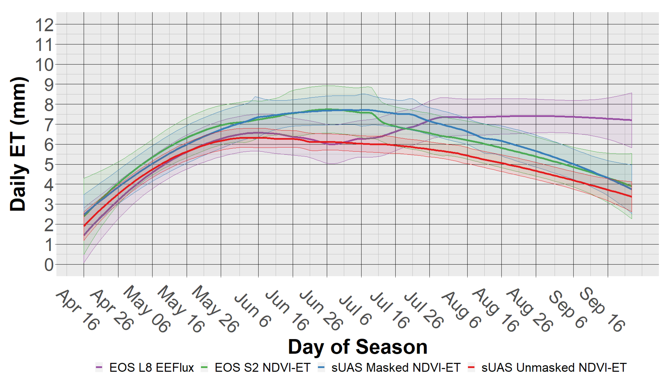
3.2. Remote Sensing of Evapotranspiration

For this study, we focused on the comparative utility of EOS and sUAS ET estimates over a single growing season (2018). We flew sUAS on ten dates April–September (Table 1), and calculated ET with EOS imagery on 20 dates (Table 2). We observe the change in daily ET over the course of the growing season (Figure 4), peaking in mid-July. During the early portion of the growing season April–June there is a close tracking relationship between NDVI-ET and EEFlux estimates, rising from 1.4 mm day 1 on 16 April to approximately 8 mm day 1 06 June. EOS observations diverge in July–September, where EEFlux estimates peak 06 August at 8.26 mm day 1 and remain high while NDVI-ET values drop after harvest. The effect of canopy masking on sUAS NDVI-ET estimates resulted in a mean positive difference of 1.23 mm day 1 ET, presumably due to fewer mixed pixels. We observe the smallest difference between masked and unmasked sUAS NDVI-ET on 19 September with a mean difference of 0.49 mm day 1 . The greatest deviation occurred on 16 July with a mean difference of 1.75 mm day 1 . Masked sUAS NDVI-ET and EOS S2 NDVI-ET estimates were often the most similar between all methods. During the season EOS ET ranged from a minimum pixel value of 0.93 mm day 1 on 16 April to the maximum 9.74 mm day 1 on 21 June. The minimum observed EOS mean daily ET of 1.45 mm day 1 occurred on 16 April using L8 EEFlux. The maximum observed EOS mean daily ET of 8.14 mm day 1 occurred on 06 August (Table 2). sUAS NDVI-ET ranged from 0.49 mm day 1 on 07 May to 8.79 mm day 1 on 16 July. Mean sUAS NDVI-ET was lowest on 19 September at 3.58 mm day 1 and greatest on 16 July at 8.04 mm day 1 .
Large irrigation events occurred on 22–23 September with a cumulative applied water of approximately 52 mm for those two days (Figure 3) coinciding with the high reported ET from EEFlux on 23 September. On 19 September observations by sUAS and EOS are much lower than observed on 23 September from EEFlux. On 19 September it had been eight days since last applied water with a noon temperature of 24.7 °C. Similarly, 23 September had a noon temperature over 5° greater at 30.5 °C.

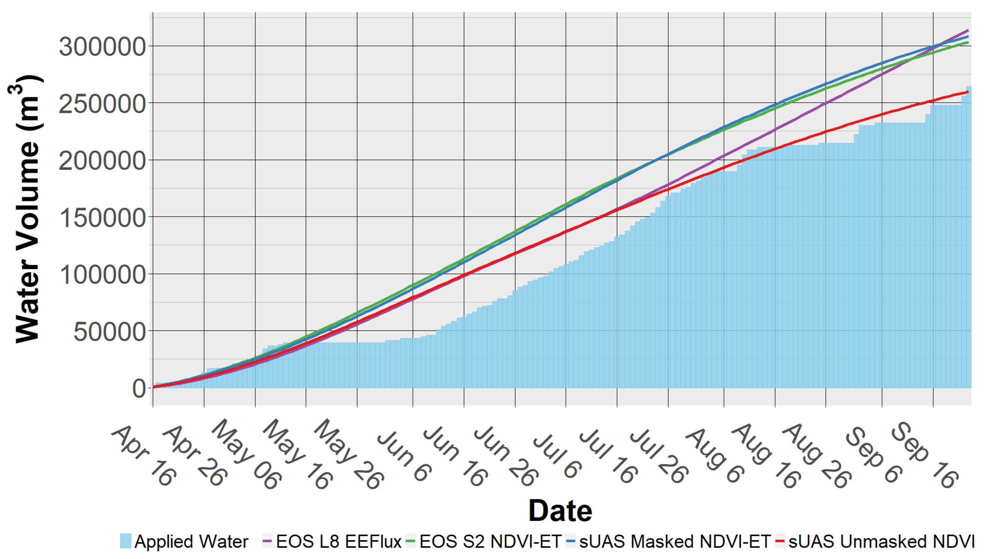
Seasonal Evapotranspiration

Mean ET a from Landsat 8 EEFlux peaks on 25 August at 7.41 mm day 1 (Figure 5). The other RSE methods peak much earlier in the season: Sentinel 2 NDVI-ET peaks on 27 June at 7.74 mm day 1 ; sUAS Masked NDVI-ET peaks on 7 July at 7.71 mm day 1 ; and sUAS Unmasked NDVI-ET peaks lower than the other methods on 3 June at 6.32 mm day 1 . Landsat 8 EEFlux and sUAS Unmasked NDVI-ET follow a similar trend until the end of June where EEFlux values rise to above 7 mm day 1 and remain there for the remainder of the season. The cumulative ET a over the growing season is shown in Figure 6. Cumulative ET a from EEFlux and sUAS Unmasked NDVI-ET are nearly the same until mid-July when EEFlux quickly rises and overtakes all other methods for a season total ET a of 313,634 m 3 (Table 3). The unmasked sUAS ET a was within 5000 m 3 of the volume of applied irrigation and was 95 percent confident within a range of 50,000 m 3 . In contrast both EOS methods had about double the range of confidence and the masked sUAS ET a was between with a range of about 80,000 m 3 .

4. Discussion

4.1. Viticultural Considerations

The application of RSE in viticulture is important for several reasons. Viticulture, the cultivation of wine and table grapes, is a global enterprise with increasing acreage globally [45]. It is increasingly challenged by changing hydroclimates and atmospheric warming. Impacts of warming atmospheric temperatures not only have the potential to affect ET in vineyards, but also impact fruit quality [46]. Observed air temperatures have increased markedly across major winegrowing regions globally [47], and winegrape growers have started to adopt adaptation strategies aimed at minimizing the harshest impacts of elevated temperature [48], namely dehydration and early ripening. One adaptation strategy is to reduce canopy temperatures through evaporative cooling from overhead misting, which would further increase total crop water use due to this additional application. Given water scarcity in many winegrape growing regions, minimizing the water footprint of viticulture is a top priority for the industry [49,50]. As such, grower-ready tools are necessary to better manage irrigation strategies. While subscription services to provide guidance on daily crop water demand are increasingly available, some growers may choose to use satellite or sUAS monitoring protocols as to control their own data and/or perform custom, on-demand analysis. RSE of vineyards has been the focus of several recent studies [51], in part due to the high commercial value of the crop and increasing sustainability practices [52]. In this study, we examined the temporal distribution of an energy balance EOS satellite based RSE approach to index-based RSE methods, including commercial-grade sUAS platforms that growers may want to employ. Our results indicate that there is general agreement between between EOS and sUAS NDVI-ET estimates and, moreover, that masking sUAS imagery to canopy pixels reduced the variance of RSE values (Figure 6) and generally conformed to the amount of applied water within the vineyard block (Figure 3). The processing of sUAS imagery is not trivial (see Montazar et al. [53] for another example), and smaller grower operations may be challenged to implement sUAS RSE on a routine basis.

4.2. RSE Considerations

The offset nature of EOS overpasses prevented a direct comparison between RSE products, and daily ET estimates especially given external factors such as weather and irrigation. Across most of the growing season we observe a similar trend between the EEFlux and NDVI-ET methods with low ET early in the season, peaking around July, then dropping back down again after harvest. Late in the season, however, EEFlux estimates remain consistent with early/mid summer values rather than a decrease to coincide with leaf senescence. We expect that later in the season, EEFlux is overestimating the actual ET due to recent irrigation applied on 22–23 September in conjunction with days 5 °C greater than 19 September during the S2 overpass and sUAS flights (Figure 3). Masking sUAS imagery yielded similar results to the EOS methods and appears to overestimate the actual amount of ET. The unmasked sUAS imagery yielded a lower estimate that was very close to the amount of applied water during the season.
As expected, soil masking increased the mean ET and decreased variance since isolating the grape canopy removed ET influence from bare soil and cover crop in the image (Table 2). We also found that the difference between masked and unmasked sUAS ET changes temporally with the largest difference occurring during peak ET in mid-July and the smallest difference after harvest. Assuming the masked sUAS ET is more representative of the real ET a , it implies that lower spatial resolution (i.e., mixed pixel) EOS RSE values are underestimating during the period of peak ET, and moreoever the EEFlux values are compromised during the end of season period that experience high air temperature, full field saturation from irrigation, and vine senescence. These observations are consistent with other studies, such as Gowda et al. [54] that showed high errors EOS RSE of post-harvest cotton, and more generally the theoretical basis by Li et al. [55] showing high estimates of ET a under saturated soil conditions and sensed high surface temperatures. We also observed large variations between the minimum and maximum RSE values (Table 2), with the lowest values attributed to the unmasked sUAS and EEFlux consistently had very high minimum values (2–3 mm day 1 higher than S2 NDVI-ET estimates). The lack of variance in EEFlux estimates could have consequences for measures of centrality and confidence for growing season totals (Table 3).

4.3. Land Use Considerations

This study focused on the use of commercial grade “off-the-shelf” approaches to sUAS RSE for the purposes of improving irrigation regimes in vineyards. The study location in California’s San Joaquin Valley has a number of concomitant land use stressors that require remediation. As new RSE and similar technologies become more readily available and deployable, it is highly likely that these technologies can be used to mitigate issues beyond water scarcity. Current over-reliance on groundwater reserves for crop applied water has stressed California’s aquifers [56]. Furthermore, other forms of agriculture have generated excess nitrogen throughout the region [57,58], which can lead to myriad impacts on environmental [59] and agroeconomic systems [60], and ultimately human well-being. Remedies in this region include enhancing viticulture in active recharge zones around groundwater dependent communities [61], constructing distributed desalination systems for brackish irrigation return water [62], incorporating wildlife friendly farming practices [63], and integrated management of forests and watersheds for clean water supply [64]. Despite current challenges in the operational deployment of sUAS [65] for environmental management, sUAS remote sensing can provide critical data to inform such land use management decisions beyond better estimates of ET, including biomass and carbon quantification for regenerative agriculture [66]. In this sense, strategic land use planning and decision making in the agricultural sector would benefit from broader adoption of sUAS technologies.

4.4. Study Limitations

A limitation of the NDVI-ET approach used here, aside from its comparative simplicity, is that it relies on external sources for ET o . While there was a nearby weather station with a similar climate and land use, the radiometer was unreliable so reference ET from a local site was unavailable. Therefore, we relied on the Spatial CIMIS daily ET o product since the nearest CIMIS stations were over 30 km away and were potentially unrepresentative of the ET o at the study site.
EOS ET estimation is limited by infrequent return times and low spatial resolution; which can be improved through the use of sUAS. Seasonal ET estimates can be heavily biased by outlying overpass dates where conditions may not represent the majority of days between the overpasses, like we observed towards the end of the season with Landsat 8. We also see that EOS estimates overestimate the actual ET for our study site. Using fine resolution sUAS imagery up-scaled to S2 resolution (10 m) reduced the mean ET a value by an average 1.233 mm for the season which accounts for a substantial volume for a large area. The EOS ET estimates are most similar to the sUAS ET when bare soil is masked out, especially during the peak of the season when the canopy is fully grown and covers most of the field area. It seems likely that the lower spatial resolution from EOS platforms leads to an overestimation of ET for vineyards as the peak ET from the canopy gets generalized for the entire cell area, which in reality contains areas with much less ET like we can observe with the sUAS imagery. Furthermore, future studies would benefit from harmonized EOS data reconciling differences in sensor sensitivity and spectral band widths [39,43].

5. Conclusions

In this study, we evaluated whether EOS and sUAS ET estimates fundamentally differ over same period of time. We showed that more traditional heat balance approaches to EOS RSE can be compromised by field conditions, such as soil saturation and excessive air temperature, and lead to overestimation of ET compared to other methods. Further, we showed that over the course of the growing season, sUAS values largely follow seasonal patterns and track EOS RSE values, but that ET variance is reduced by isolating canopy pixels. While EOS and sUAS ET estimates do not fundamentally differ over the same study domain and same period of time, comparing upscaled sUAS ET to EOS ET estimates within and across pixels, we showed that unmasked high resolution sUAS ET estimates have the highest variance but that EOS EEFlux ET values have high variance too. These “mixed pixels” inherent in EOS data obscure important signals in ET estimation through inclusion of soil fraction, and given that vineyards change over the course of a growing season in terms of biomass and leaf area index can change, caution should be used when evaluating ET whether using traditional energy balance models or RSE proxies. These findings can provide growers with guidance on their own use of new RSE products and sUAS platforms for calibration and verification.

Author Contributions

Conceptualization, J.H.V.; Methodology, J.H.V., M.K., A.M.R., J.M.-A.; Software, M.K., A.M.R., L.B.; Formal Analysis, J.H.V., M.K., A.M.R.; Resources, J.H.V., J.M.-A., S.C.; Investigation, J.H.V., M.K., A.M.R., L.B.; Writing—original draft preparation, J.H.V., M.K.; Writing—review and editing, J.H.V., M.K., A.M.R., J.M.-A., S.C.; Visualization, J.H.V., M.K., A.M.R.; Supervision, J.H.V., A.M.R.; Project Administration, J.H.V., A.M.R., S.C.; Funding Acquisition, J.H.V., J.M.-A., S.C. All authors have read and agreed to the published version of the manuscript.

Funding

This research was partially supported by the National Robotics Initiative (NRI) grant no. 2017-67021-25925 from the USDA National Institute of Food and Agriculture. Any opinions, findings, conclusions, or recommendations expressed in this publication are those of the author(s) and do not necessarily reflect the view of the U.S. Department of Agriculture. Lorenzo Booth was partially supported by the NSF under grant DGE-1633722. Any opinions, findings, conclusions, or recommendations expressed in this publication are those of the authors and do not necessarily reflect the view of NSF. Additional support was from the Public Policy Institute of California (PPIC) Steyer-Taylor Fellowship and the UC Merced Center for Information Technology Research in the Interest of Society (CITRIS) and CITRIS Aviation.

Acknowledgments

We gratefully acknowledge the lab and field assistance of Andreas Anderson, and support from Brandon Stark of the University of California Drone Safety Center. We thank E. & J. Gallo Winery for access to the site, and their science team of Nick Dokoozlian, Maria Mar Alsina, Brent Sams and Luis A. Sanchez for insights to the study system.

Conflicts of Interest

The authors declare no conflict of interest.

References

  1. Vörösmarty, C.J.; Sahagian, D. Anthropogenic disturbance of the terrestrial water cycle. Bioscience 2000, 50, 753–765. [Google Scholar]
  2. Vörösmarty, C.J.; Green, P.; Salisbury, J.; Lammers, R.B. Global water resources: Vulnerability from climate change and population growth. Science 2000, 289, 284–288. [Google Scholar] [CrossRef] [PubMed] [Green Version]
  3. Yeh, P.J.F.; Famiglietti, J. Regional terrestrial water storage change and evapotranspiration from terrestrial and atmospheric water balance computations. J. Geophys. Res. Atmos. 2008, 113. [Google Scholar] [CrossRef]
  4. Vörösmarty, C.J.; McIntyre, P.B.; Gessner, M.O.; Dudgeon, D.; Prusevich, A.; Green, P.; Glidden, S.; Bunn, S.E.; Sullivan, C.A.; Liermann, C.R.; et al. Global threats to human water security and river biodiversity. Nature 2010, 467, 555–561. [Google Scholar] [CrossRef] [PubMed]
  5. Wisser, D.; Frolking, S.; Douglas, E.M.; Fekete, B.M.; Vörösmarty, C.J.; Schumann, A.H. Global irrigation water demand: Variability and uncertainties arising from agricultural and climate data sets. Geophys. Res. Lett. 2008, 35. [Google Scholar] [CrossRef] [Green Version]
  6. Berni, J.; Zarco-Tejada, P.J.; Suárez, L.; González-Dugo, V.; Fereres, E. Remote sensing of vegetation from UAV platforms using lightweight multispectral and thermal imaging sensors. Int. Arch. Photogramm. Remote Sens. Spatial Inform. Sci. 2009, 38, 6. [Google Scholar] [CrossRef]
  7. Zhang, C.; Kovacs, J.M. The application of small unmanned aerial systems for precision agriculture: A review. Precis. Agric. 2012, 13, 693–712. [Google Scholar] [CrossRef]
  8. Nassar, A.; Torres-Rua, A.; Kustas, W.; Nieto, H.; McKee, M.; Hipps, L.; Stevens, D.; Alfieri, J.; Prueger, J.; Alsina, M.M.; et al. Influence of Model Grid Size on the Estimation of Surface Fluxes Using the Two Source Energy Balance Model and sUAS Imagery in Vineyards. Remote. Sens. 2020, 12, 342. [Google Scholar] [CrossRef] [Green Version]
  9. Peter, B.G.; Messina, J.P.; Carroll, J.W.; Zhi, J.; Chimonyo, V.; Lin, S.; Snapp, S.S. Multi-Spatial Resolution Satellite and sUAS Imagery for Precision Agriculture on Smallholder Farms in Malawi. Photogramm. Eng. Remote Sens. 2020, 86, 107–119. [Google Scholar] [CrossRef]
  10. Ritchie, H.; Roser, M. Water Use and Stress. Our World in Data. 2017. Available online: https://ourworldindata.org/water-use-stress (accessed on 28 September 2020).
  11. Underwood, E.C.; Viers, J.H.; Klausmeyer, K.R.; Cox, R.L.; Shaw, M.R. Threats and biodiversity in the mediterranean biome. Divers. Distrib. 2009, 15, 188–197. [Google Scholar] [CrossRef]
  12. Grantham, T.E.; Viers, J.H. 100 years of California’s water rights system: Patterns, trends and uncertainty. Environ. Res. Lett. 2014, 9, 084012. [Google Scholar] [CrossRef]
  13. United States Department of Agriculture. 2017 Census of Agriculture, United States Summary and State Data; Volume 1, Geographic Area Series, Part 51, AC-17-A-51; Technical Report; National Agricultural Statistics Service (USDA): Washington, DC, USA, 2019. Available online: https://www.nass.usda.gov/Publications/AgCensus/2017/Full_Report/Volume_1,_Chapter_1_US/ (accessed on 28 September 2020).
  14. Sabo, J.L.; Sinha, T.; Bowling, L.C.; Schoups, G.H.; Wallender, W.W.; Campana, M.E.; Cherkauer, K.A.; Fuller, P.L.; Graf, W.L.; Hopmans, J.W.; et al. Reclaiming freshwater sustainability in the Cadillac Desert. Proc. Natl. Acad. Sci. USA 2010, 107, 21263–21269. [Google Scholar] [CrossRef] [PubMed] [Green Version]
  15. Hoekstra, A.Y.; Mekonnen, M.M.; Chapagain, A.K.; Mathews, R.E.; Richter, B.D. Global Monthly Water Scarcity: Blue Water Footprints versus Blue Water Availability. PLoS ONE 2012, 7. [Google Scholar] [CrossRef] [PubMed]
  16. Swain, D.L.; Tsiang, M.; Haugen, M.; Singh, D.; Charland, A.; Rajaratnam, B.; Diffenbaugh, N.S. The extraordinary California drought of 2013/2014: Character, context, and the role of climate change. Bull. Am. Meteorol. Soc. 2014, 95, S3–S7. [Google Scholar]
  17. Swain, D.L.; Langenbrunner, B.; Neelin, J.D.; Hall, A. Increasing precipitation volatility in twenty-first-century California. Nat. Clim. Chang. 2018, 8, 427–433. [Google Scholar] [CrossRef]
  18. Nover, D.; Dogan, M.; Ragatz, R.; Booth, L.; Medellín-Azuara, J.; Lund, J.; Viers, J. Does More Storage Give California More Water? JAWRA J. Am. Water Resour. Assoc. 2019, 55, 759–771. [Google Scholar] [CrossRef]
  19. Medellín-Azuara, J.; Paw, U.K.T.; Jin, Y.; Jankowski, J.; Bell, A.; Kent, E.; Clay, J.; Wong, A.; Alexander, N.; Santos, N.; et al. A Comparative Study for Estimating Crop Evapotranspiration in the Sacramento-San Joaquin Delta; Technical Report; Center for Watershed Sciences, University of California: Davis, CA, USA, 2018; Available online: https://watershed.ucdavis.edu/delta-et (accessed on 6 October 2020).
  20. Gleick, P.H. Roadmap for sustainable water resources in southwestern North America. Proc. Natl. Acad. Sci. USA 2010, 107, 21300–21305. [Google Scholar] [CrossRef] [Green Version]
  21. Yazdi, A.B.; Araghinejad, S.; Nejadhashemi, A.P.; Tabrizi, M.S. Optimal water allocation in irrigation networks based on real time climatic data. Agric. Water Manag. 2013, 117, 1–8. [Google Scholar]
  22. Zaks, D.P.; Kucharik, C.J. Data and monitoring needs for a more ecological agriculture. Environ. Res. Lett. 2011, 6, 014017. [Google Scholar] [CrossRef]
  23. Wang, K.; Dickinson, R.E. A review of global terrestrial evapotranspiration: Observation, modeling, climatology, and climatic variability. Rev. Geophys. 2012, 50. [Google Scholar] [CrossRef]
  24. Liou, Y.A.; Kar, S.K. Evapotranspiration estimation with remote sensing and various surface energy balance algorithms—A review. Energies 2014, 7, 2821–2849. [Google Scholar] [CrossRef] [Green Version]
  25. Zhang, K.; Kimball, J.S.; Running, S.W. A review of remote sensing based actual evapotranspiration estimation. Wiley Interdiscip. Rev. Water 2016, 3, 834–853. [Google Scholar] [CrossRef]
  26. Bastiaanssen, W.G.; Menenti, M.; Feddes, R.; Holtslag, A. A remote sensing surface energy balance algorithm for land (SEBAL). 1. Formulation. J. Hydrol. 1998, 212, 198–212. [Google Scholar] [CrossRef]
  27. Bastiaanssen, W.G.; Pelgrum, H.; Wang, J.; Ma, Y.; Moreno, J.; Roerink, G.; Van der Wal, T. A remote sensing surface energy balance algorithm for land (SEBAL): Part 2: Validation. J. Hydrol. 1998, 212, 213–229. [Google Scholar] [CrossRef]
  28. Bastiaanssen, W.; Noordman, E.; Pelgrum, H.; Davids, G.; Thoreson, B.; Allen, R. SEBAL model with remotely sensed data to improve water-resources management under actual field conditions. J. Irrig. Drain. Eng. 2005, 131, 85–93. [Google Scholar] [CrossRef]
  29. Allen, R.G.; Tasumi, M.; Trezza, R. Satellite-based energy balance for mapping evapotranspiration with internalized calibration (METRIC)—Model. J. Irrig. Drain. Eng. 2007. [Google Scholar] [CrossRef]
  30. Irmak, A.; Allen, R.G.; Kjaersgaard, J.; Huntington, J.; Kamble, B.; Trezza, R.; Ratcliffe, I. Operational Remote Sensing of ET and Challenges. In Evapotranspiration; Irmak, A., Ed.; IntechOpen: Rijeka, Croatia, 2012; Chapter 21. [Google Scholar] [CrossRef] [Green Version]
  31. Morton, C.; Harding, J.; Erickson, T. OpenET: Filling the Biggest Gap in Water Management. Available online: https://github.com/Open-ET (accessed on 28 September 2020).
  32. Mitchell, K.E.; Lohmann, D.; Houser, P.R.; Wood, E.F.; Schaake, J.C.; Robock, A.; Cosgrove, B.A.; Sheffield, J.; Duan, Q.; Luo, L.; et al. The multi-institution North American Land Data Assimilation System (NLDAS): Utilizing multiple GCIP products and partners in a continental distributed hydrological modeling system. J. Geophys. Res. Atmos. 2004, 109. [Google Scholar] [CrossRef] [Green Version]
  33. Xia, Y.; Mitchell, K.; Ek, M.; Sheffield, J.; Cosgrove, B.; Wood, E.; Luo, L.; Alonge, C.; Wei, H.; Meng, J.; et al. Continental-scale water and energy flux analysis and validation for the North American Land Data Assimilation System project phase 2 (NLDAS-2): 1. Intercomparison and application of model products. J. Geophys. Res. Atmos. 2012, 117. [Google Scholar] [CrossRef]
  34. Abatzoglou, J.T. Development of gridded surface meteorological data for ecological applications and modelling. Int. J. Climatol. 2013, 33, 121–131. [Google Scholar] [CrossRef]
  35. Stark, B.; Smith, B.; Chen, Y. Survey of thermal infrared remote sensing for Unmanned Aerial Systems. In Proceedings of the 2014 International Conference on Unmanned Aircraft Systems (ICUAS), Orlando, FL, USA, 27–30 May 2014; IEEE: New York, NY, USA, 2014; pp. 1294–1299. [Google Scholar]
  36. Zhao, T.; Niu, H.; Anderson, A.; Chen, Y.; Viers, J. A detailed study on accuracy of uncooled thermal cameras by exploring the data collection workflow. In Proceedings of the Autonomous Air and Ground Sensing Systems for Agricultural Optimization and Phenotyping III. International Society for Optics and Photonics, Orlando, FL, USA, 16–17 April 2018; Volume 10664, p. 106640F. [Google Scholar]
  37. Torres-Rua, A. Vicarious calibration of sUAS microbolometer temperature imagery for estimation of radiometric land surface temperature. Sensors 2017, 17, 1499. [Google Scholar] [CrossRef] [Green Version]
  38. Roche, J.W.; Ma, Q.; Rungee, J.; Bales, R.C. Evapotranspiration Mapping for Forest Management in California’s Sierra Nevada. Front. For. Glob. Chang. 2020, 3, 69. [Google Scholar] [CrossRef]
  39. Scheffler, D.; Frantz, D.; Segl, K. Spectral harmonization and red edge prediction of Landsat-8 to Sentinel-2 using land cover optimized multivariate regressors. Remote Sens. Environ. 2020, 241, 111723. [Google Scholar] [CrossRef]
  40. Hart, Q.J.; Brugnach, M.; Temesgen, B.; Rueda, C.; Ustin, S.L.; Frame, K. Daily reference evapotranspiration for California using satellite imagery and weather station measurement interpolation. Civ. Eng. Environ. Syst. 2009, 26, 19–33. [Google Scholar] [CrossRef]
  41. Rigollier, C.; Lefèvre, M.; Cros, S.; Wald, L. Heliosat 2: An improved method for the mapping of the solar radiation from Meteosat imagery. In Proceedings of the EUMETSAT Meteorological Satellite Conference, Dublin, Ireland, 1–6 September 2002; EUMETSAT: Darmstadt, Germany, 2002; pp. 585–592. [Google Scholar]
  42. Walter, I.A.; Allen, R.G.; Elliott, R.; Jensen, M.E.; Itenfisu, D.; Mecham, B.; Howell, T.A.; Snyder, R.; Brown, P.; Echings, S.; et al. The ASCE Standardized Reference Evapotranspiration Equation; Rep. 0-7844-0805-X, ASCE Task Committee on Standardization of Reference Evapotranspiration; ASCE: Reston, VA, USA, 1977. [Google Scholar]
  43. Claverie, M.; Ju, J.; Masek, J.G.; Dungan, J.L.; Vermote, E.F.; Roger, J.C.; Skakun, S.V.; Justice, C. The Harmonized Landsat and Sentinel-2 surface reflectance data set. Remote. Sens. Environ. 2018, 219, 145–161. [Google Scholar] [CrossRef]
  44. Zhang, W.; Qi, J.; Wan, P.; Wang, H.; Xie, D.; Wang, X.; Yan, G. An easy-to-use airborne LiDAR data filtering method based on cloth simulation. Remote. Sens. 2016, 8, 501. [Google Scholar] [CrossRef]
  45. Viers, J.H.; Williams, J.N.; Nicholas, K.A.; Barbosa, O.; Kotzé, I. Vinecology: Pairing wine with nature. Conserv. Lett. 2013, 6, 287–299. [Google Scholar] [CrossRef]
  46. Van Leeuwen, C.; Darriet, P. The impact of climate change on viticulture and wine quality. J. Wine Econ. 2016, 11, 150–167. [Google Scholar] [CrossRef] [Green Version]
  47. Jones, G.V.; White, M.A.; Cooper, O.R.; Storchmann, K. Climate change and global wine quality. Clim. Chang. 2005, 73, 319–343. [Google Scholar] [CrossRef]
  48. Nicholas, K.A.; Durham, W.H. Farm-scale adaptation and vulnerability to environmental stresses: Insights from winegrowing in Northern California. Glob. Environ. Chang. 2012, 22, 483–494. [Google Scholar] [CrossRef]
  49. Costa, J.; Vaz, M.; Escalona, J.; Egipto, R.; Lopes, C.; Medrano, H.; Chaves, M. Modern viticulture in southern Europe: Vulnerabilities and strategies for adaptation to water scarcity. Agric. Water Manag. 2016, 164, 5–18. [Google Scholar] [CrossRef]
  50. Herath, I.; Green, S.; Singh, R.; Horne, D.; van der Zijpp, S.; Clothier, B. Water footprinting of agricultural products: A hydrological assessment for the water footprint of New Zealand’s wines. J. Clean. Prod. 2013, 41, 232–243. [Google Scholar] [CrossRef]
  51. Kustas, W.P.; Agam, N.; Ortega-Farias, S. Forward to the GRAPEX special issue. Irrig. Sci. 2019, 37, 221–226. [Google Scholar] [CrossRef] [Green Version]
  52. Santiago-Brown, I.; Metcalfe, A.; Jerram, C.; Collins, C. Sustainability assessment in wine-grape growing in the new world: Economic, environmental, and social indicators for agricultural businesses. Sustainability 2015, 7, 8178–8204. [Google Scholar] [CrossRef] [Green Version]
  53. Montazar, A.; Krueger, R.; Corwin, D.; Pourreza, A.; Little, C.; Rios, S.; Snyder, R.L. Determination of Actual Evapotranspiration and Crop Coefficients of California Date Palms Using the Residual of Energy Balance Approach. Water 2020, 12, 2253. [Google Scholar] [CrossRef]
  54. Gowda, P.H.; Chávez, J.L.; Howell, T.A.; Marek, T.H.; New, L.L. Surface energy balance based evapotranspiration mapping in the Texas high plains. Sensors 2008, 8, 5186–5201. [Google Scholar] [CrossRef]
  55. Li, Z.L.; Tang, R.; Wan, Z.; Bi, Y.; Zhou, C.; Tang, B.; Yan, G.; Zhang, X. A review of current methodologies for regional evapotranspiration estimation from remotely sensed data. Sensors 2009, 9, 3801–3853. [Google Scholar] [CrossRef] [Green Version]
  56. Medellín-Azuara, J.; MacEwan, D.; Howitt, R.E.; Koruakos, G.; Dogrul, E.C.; Brush, C.F.; Kadir, T.N.; Harter, T.; Melton, F.; Lund, J.R. Hydro-economic analysis of groundwater pumping for irrigated agriculture in California’s Central Valley, USA. Hydrogeol. J. 2015, 23, 1205–1216. [Google Scholar] [CrossRef]
  57. Rosenstock, T.; Liptzin, D.; Dzurella, K.; Fryjoff-Hung, A.; Hollander, A.; Jensen, V.; King, A.; Kourakos, G.; McNally, A.; Stuart Pettygrove, G.; et al. Agriculture’s contribution to nitrate contamination of Californian groundwater (1945–2005). J. Environ. Qual. 2014, 43. [Google Scholar] [CrossRef] [Green Version]
  58. Lockhart, K.M.; King, A.M.; Harter, T. Identifying sources of groundwater nitrate contamination in a large alluvial groundwater basin with highly diversified intensive agricultural production. J. Contam. Hydrol. 2013, 151, 140–154. [Google Scholar] [CrossRef]
  59. Zhang, Y.; Luo, P.; Zhao, S.; Kang, S.; Wang, P.; Zhou, M.; Lyu, J. Control and remediation methods for eutrophic lakes in the past 30 years. Water Sci. Technol. 2020, 81, 1099–1113. [Google Scholar] [CrossRef]
  60. Medellín-Azuara, J.; Rosenstock, T.S.; Howitt, R.E.; Harter, T.; Jessoe, K.K.; Dzurella, K.; Pettygrove, S.; Lund, J.R. Agroeconomic analysis of nitrate crop source reductions. J. Water Resour. Plan. Manag. 2013, 139, 501–511. [Google Scholar] [CrossRef]
  61. Mayzelle, M.; Viers, J.; Medellín-Azuara, J.; Harter, T. Economic feasibility of irrigated agricultural land use buffers to reduce groundwater nitrate in rural drinking: Water sources. Water 2015, 7, 12–37. [Google Scholar] [CrossRef] [Green Version]
  62. Welle, P.; Medellín-Azuara, J.; Viers, J.; Mauter, M. Economic and policy drivers of agricultural water desalination in California’s central valley. Agric. Water Manag. 2017, 194. [Google Scholar] [CrossRef]
  63. Underwood, E.; Hutchinson, R.; Viers, J.; Kelsey, T.; Distler, T.; Marty, J. Quantifying trade-offs among ecosystem services, biodiversity, and agricultural returns in an agriculturally dominated landscape under future land-management scenarios. San Franc. Estuary Watershed Sci. 2017, 15. [Google Scholar] [CrossRef] [Green Version]
  64. Luo, P.; Zhou, M.; Deng, H.; Lyu, J.; Cao, W.; Takara, K.; Nover, D.; Geoffrey Schladow, S. Impact of forest maintenance on water shortages: Hydrologic modeling and effects of climate change. Sci. Total Environ. 2018, 615, 1355–1363. [Google Scholar] [CrossRef]
  65. Hardin, P.J.; Lulla, V.; Jensen, R.R.; Jensen, J.R. Small Unmanned Aerial Systems (sUAS) for environmental remote sensing: Challenges and opportunities revisited. GIScience Remote. Sens. 2019, 56, 309–322. [Google Scholar] [CrossRef]
  66. Morandé, J.; Stockert, C.; Liles, G.; Williams, J.; Smart, D.; Viers, J. From berries to blocks: Carbon stock quantification of a California vineyard. Carbon Balance Manag. 2017, 12. [Google Scholar] [CrossRef] [Green Version]
Figure 1. Comparison of wavelength channel position and widths by sensor platform (RE = RedEdge; L8 = Landsat 8; S2 = Sentinel 2), showing a typical percent reflectance spectral response signature for a grapevine (black).
Remotesensing 12 03251 g001
Figure 2. Site map of Ripperdan 760 Block in Madera County, California, USA.
Remotesensing 12 03251 g002
Figure 3. Daily air temperature °C (right axis) for the 2018 growing season is shown for mid-day (red line) as well as maxima-minima (gray band). Applied irrigation for each day in mm (left axis) is shown as blue bars.
Remotesensing 12 03251 g003
Figure 4. Daily Evapotranspiration (ET) in mm (x-axis) ridgeline density plot for each overpass date (y-axis) comparing each method used. Landsat 8 EEFlux is colored red, Sentinel 2 NDVI-ET is shown in orange, sUAS unmasked NDVI-ET is light blue, and sUAS masked NDVI-ET is green.
Remotesensing 12 03251 g004
Figure 5. Seasonal Daily ET a in mm (y-axis) interpolated from loess model fit. Landsat 8 EEFlux is colored purple, Sentinel 2 NDVI-ET is shown in green, sUAS masked NDVI-ET is blue, and sUAS unmasked NDVI-ET is red.
Remotesensing 12 03251 g005
Figure 6. Cumulative ET a in m 3 (y-axis) interpolated from loess model fit. Landsat 8 EEFlux is colored purple, Sentinel 2 NDVI-ET is shown in green, sUAS masked NDVI-ET is blue, and sUAS unmasked NDVI-ET is red. Cumulative Applied Water from irrigation is shown in light blue columns.
Remotesensing 12 03251 g006
Table 1. Flight dates and platforms.
2018 Flight DatessUAS PlatformsUAS SensorEOS
20 AprilFinwing SabreParrot SequoiaN/A
7 MayFinwing SabreParrot SequoiaSentinel 2
6 JuneDJI S1000Micasense RedEdge-MSentinel 2
21 JuneDJI S1000Micasense RedEdge-MSentinel 2
5 JulyDJI S1000Micasense RedEdge-MLandsat 8
16 JulyDJI S1000Micasense RedEdge-MSentinel 2
26 JulyDJI S1000Micasense RedEdge-MSentinel 2
6 AugustDJI S1000Micasense RedEdge-MLandsat 8
20 AugustDJI S1000Micasense RedEdge-MSentinel 2
19 SeptemberDJI S1000Micasense RedEdge-MSentinel 2
Table 2. Summary of ET (mm) estimates from sUAS and EOS observation for 2018.
DateMethodMeanMedianStd DevVarMinMax
16 AprilEOS L8 EEFlux1.4481.3750.3400.1160.9303.265
20 AprilsUAS Unmasked NDVI-ET2.4502.5240.4180.1750.1023.688
22 AprilEOS S2 NDVI-ET3.2583.3390.4270.1821.2274.765
2 MayEOS L8 EEFlux3.8894.0160.4670.2182.3764.559
7 MaysUAS Unmasked NDVI-ET5.1545.4210.9720.9440.4856.400
EOS S2 NDVI-ET5.9086.1970.9250.8551.6356.963
18 MayEOS L8 EEFlux6.0176.1940.5820.3384.0306.654
27 MayEOS S2 NDVI-ET6.5706.9311.0511.1041.6597.425
3 JuneEOS L8 EEFlux7.5817.8050.7190.5164.9468.398
6 JunesUAS Unmasked NDVI-ET6.4656.8071.141.2990.5687.496
sUAS Masked NDVI-ET7.3087.5330.8090.6540.5237.824
EOS S2 NDVI-ET7.5677.9661.0701.1452.588.465
19 JuneEOS L8 EEFlux5.3735.5210.5490.3012.8566.035
21 JunesUAS Unmasked NDVI-ET6.1926.4931.0621.1271.1717.803
sUAS Masked NDVI-ET7.7717.8860.5900.3481.7048.423
EOS S2 NDVI-ET7.4307.7901.1061.2231.6669.743
5 JulysUAS Unmasked NDVI-ET5.7436.0250.9830.9661.1436.829
sUAS Masked NDVI-ET7.3437.4440.5540.3070.8427.884
EOS L8 EEFlux6.1426.3070.6630.4403.6696.959
16 JulysUAS Unmasked NDVI-ET6.2916.6081.1051.2201.1347.801
sUAS Masked NDVI-ET8.0388.1270.5050.2551.0228.788
EOS S2 NDVI-ET7.477.8221.071.1442.298.695
21 JulyEOS L8 EEFlux6.7876.9170.6820.4654.4887.783
26 JulysUAS Unmasked NDVI-ET5.6245.9251.0361.0740.8996.816
sUAS Masked NDVI-ET6.8217.0350.8710.7580.8097.562
EOS S2 NDVI-ET5.9416.1830.7340.5392.3646.817
6 AugustsUAS Unmasked NDVI-ET5.3725.6331.0021.0050.7686.753
sUAS Masked NDVI-ET6.6096.760.6940.4820.8727.326
EOS L8 EEFlux8.1358.2640.6750.4555.5979.18
20 AugustsUAS Unmasked NDVI-ET4.9065.1460.8750.7650.8816.739
sUAS Masked NDVI-ET6.086.1910.5840.3420.837.297
EOS S2 NDVI-ET5.9316.1510.7970.6352.0498.094
22 AugustEOS L8 EEFlux6.7996.7070.5410.2935.6128.111
7 SeptemberEOS L8 EEFlux7.0437.2310.7280.5304.4968.328
19 SeptembersUAS Unmasked NDVI-ET3.5773.7500.6770.4580.6144.641
sUAS Masked NDVI-ET4.0664.1980.6130.3760.7334.968
EOS S2 NDVI-ET4.0884.2390.6650.4431.0825.636
23 SeptemberEOS L8 EEFlux7.4667.7060.6280.3944.9988.165
Table 3. Cumulative ET (10 3 m 3 ) with 95% confidence interval bounds, and applied irrigation, for 2018 growing season.
MethodLower BoundMeanUpper Bound
sUAS Unmasked NDVI-ET237.29259.81282.32
sUAS Masked NDVI-ET267.64308.13348.62
EOS S2 NDVI-ET249.61303.21356.81
EOS L8 EEFlux266.83313.63360.44
Applied Irrigation 264.34

