1. Introduction
The existence of pre-earthquake anomalous phenomena is a highly controversial issue in the scientific community [
1,
2,
3,
4]. This debate exists mainly because these phenomena generally pass statistical tests, but they originate from unknown sources [
5,
6,
7]. Atmospheric acoustic-gravity waves have been considered as one of the factors that induce changes in ionospheric density, which could cause seismo-ionospheric perturbations before earthquakes [
8,
9,
10,
11,
12]. However, seeking seismic-related vibration sources such as crustal displacements [
13,
14,
15,
16,
17,
18] and ground motion occurring before earthquakes has remained a great challenge until the present. On 6 February 2016, the M6.6 Meinong earthquake (22.92° N, 120.54° E) occurred in southern Taiwan (
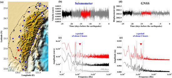
Figure 1a), causing the loss of hundreds of lives [
19]. The continuous seismic data recorded by the broadband seismometer at the B770 (22.54°N, 120.39°E) station, which is operated by National Center for Research on Earthquake Engineering (NCREE) of Taiwan, show that variations in the amplitude of ground velocity doubled from the background noise level (i.e., the double-amplitude vibrations) for 10–15 days before the earthquake (
Figure 1b). Spectra of the double-amplitude vibrations were mainly distributed at frequencies near 1.4 × 10
−4 Hz (a period of 2 h) (
Figure 1c). These amplifications lasted for 10 days and became minimal within a few days after the earthquake’s occurrence (
Figure S1). We chose the seismic data recorded approximately 100 days before the earthquake for examining whether the existence of the amplification is permanent or provisional.
Figure 1c shows that the associated amplification cannot be observed approximately 100 days before the earthquake. The result suggests that the amplifications are not permanent but could be pre-earthquake anomalous phenomena associated with the Meinong earthquake. Note that the behavior of the associated amplification at frequencies near 1.4 × 10
−4 Hz is distinct from that of slow earthquakes, microcracks, and tremors, which are observed at relatively high frequencies (0.1–10 Hz) [
19,
20,
21,
22].
Surface displacements monitored by using the ground-based Global Navigation Satellite Systems (GNSS) data can exhibit similar elastic deformation and/or oscillation in the spatiotemporal domain if the double-amplitude vibrations actually exist. Vertical displacements retrieved from ground-based GNSS receivers were taken into consideration to examine whether the double-amplitude vibrations in seismic records are affected by dynamic ranges at such low frequencies (i.e., a cycle of near 2 h). The GNSS data in Taiwan were provided by the Geophysical Database Management System of the Central Weather Bureau [
23]. However, parts of the stations only record the Global Positioning System (GPS) observations. For the consistency of the data processing, only GPS observations were taken into account in this study. A total of thirty-six GNSS stations were selected, and the Canadian Spatial Reference System (CSRS) Precise Point Positioning (PPP) online computation system was utilized to calculate the 3D coordinates of the GNSS stations. The CSRS-PPP system uses the precise GNSS satellite orbit ephemerides; therefore, the coordinates in this study were taken from the International Terrestrial Reference Frame 2014. Moreover, the kinematic mode was adopted in the data processing and the coordinates were produced every 30 s. To increase the accuracy of the data processing, an ocean tide loading correction was applied and the NAO.99b model was used to obtain the optimal correction effect [
24]. The amplification can also be found in the vertical component of the GNSS data at the LGUE (22.99°N, 120.54°E) station between 10 days and 15 days before the earthquake (
Figure 1d,e). The amplification exhibits that the Earth’s surface oscillates vertically with an amplitude of approximately 0.1 m with a cycle period of approximately 2 h. The oscillation shares similar characteristics in the frequency (i.e., near 1.4 × 10
−4 Hz) and the occurring time with those signals in the seismic velocity data (
Figure 1d,e). Meanwhile, an average rate close to 6.17 × 10
−6 m/s derived from the associated oscillation of the Earth’s surface also shows an agreement with the seismic data. Note that the frequency of the amplification is different compared with the well-known frequency-dependent effects (such as the lunar elliptic tides, lunar semi-diurnal tides, lunar-solar semi-diurnal tides and so on) on the surface displacements [
25,
26].
2. Methodology
To understand the spatiotemporal distribution of the double-amplitude vibrations associated with the earthquake, we collected seismic ground velocity data at the thirty-one stations, which are operated by NCREE, and the GNSS data in Taiwan. The background amplitude was computed by utilizing the data in the frequency band of interest (i.e., from 8 × 10⁻⁵ to 2 × 10⁻⁴ Hz) within a time span of 0–60 days before the earthquake for each station using the Fourier transform. In contrast, the monitoring amplitude was computed by using the data in the same frequency band within a moving window spanning 5 days from 25 to 0 days before the earthquake. The amplification ratio was calculated by dividing the monitoring amplitude by the background amplitude. Spatial distributions of the amplification ratios were obtained by applying a gridding method for the amplification ratios of all the stations.
Furthermore, we utilized the data at two horizontal components in each station to evaluate the azimuth of wave propagation (excited by the ground vibrations) using the maximum horizontal amplitude [
27] for further determining location sources of the ground vibrations. Areas that potentially reveal the locations of sources were defined by using a sector centered on the propagation azimuth with an expansion angle of 15° on both sides. This implies a resolution of 30° in the determination of the propagation azimuth. The radius of a sector was determined to be 300 km because enhancements of 10–20% were distributed in areas covering the whole Taiwan island. The locations of sources were determined by using intersectional areas of the sectors, which overlapped at least three stations with significant enhancements.
On the other hand, once the multiple stations detected the double-amplitude vibrations, the principal component analysis (PCA) method [
28] was also employed to extract common-mode ground vibrations from the thirty-one seismic stations in Taiwan during the Meinong earthquake. The ground velocity data within a time span of one year from all the seismic stations were filtered by using a bandpass filter of 8 × 10
−5–2 × 10
−4 Hz (i.e., a period of 1.5–3.5 h). Strong peak values, which are caused by unwanted influences (i.e., artificial noise, local earthquakes, teleseismic waves and so on), were mitigated through the summation of the filtered amplitudes as a daily value [
29]. The summated daily values at all the stations were processed through the PCA method, to extract common-mode ground vibrations during the Meinong earthquake. The PCA method is a statistical procedure that widely utilizes an orthogonal transformation to convert a set of observations of possibly correlated variables into a set of linearly uncorrelated variables called principal components [
28]. The first principal component retrieved from the PCA method was determined as the common-mode ground vibrations that were further compared with other potential interferences to clarify the causal mechanism. Finally, Molchan’s error diagram [
30] was utilized to evaluate the prediction performance of the phenomena of the common-mode ground vibrations for earthquake forecasting. Molchan’s error diagram can evaluate the prediction curve via the rate of earthquakes detected against the rate of alarming cells. Notably, a modified area skill score measured the area between the actual prediction curve and the random prediction line that is conducted in Molchan’s error diagram. The scores above zero indicated that the prediction is better than the random and the observation contained precursory information. We show the flow chart in
Figure 2.
3. The Spatiotemporal Distribution and the Source Location of the Vibrations
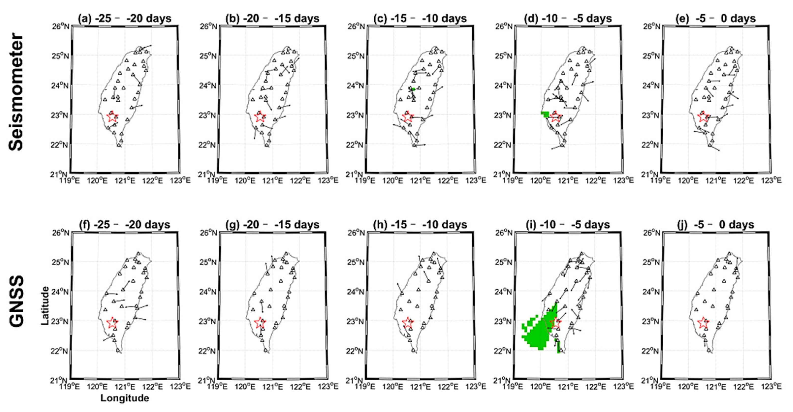
The amplification ratio of the vertical seismic data was near one for 10 days before the earthquake (
Figure 3a–c). In contrast, the amplification ratio significantly enhanced to close to 2 and was widely distributed in the area entirely covering Taiwan about 5–10 days before the earthquake (
Figure 3d). In terms of 0–5 days before the earthquake, the enhancements gradually attenuated in the whole study area, except for a local region in the southern part of Taiwan (
Figure 3e). Regarding the amplification ratio of the vertical displacement of the GNSS data, the ratios were roughly near 1 for approximately 10–25 days before the earthquake (
Figure 3f–h). The ratios obviously enhanced to 2 about 10 days before the earthquake that roughly covered the whole Taiwan island (
Figure 3i). Similarly, the ratios attenuated to about 1 and were comparable with the background (i.e., 10-25 days before the earthquake) for 0–5 days before the earthquake. In short, consistent behaviors related to the changes in time-variant spatial distributions can be seen in the GNSS data (
Figure 3f–j). The amplification ratio near 2 distributes in a wide area that is significantly larger than the fault rupture zone of the earthquake about 5–10 days before the event. However, the boundary of the enhancements is vague due to the limitation posed by the land area of Taiwan.
In
Figure 4, we further discuss the source location of the enhancements associated with the ground vibrations. No obvious source location can be observed 15 days before the earthquake from either seismic (
Figure 4a–c) or GNSS (
Figure 4f–h) data due to insignificant enhancements (
Figure 3a–c and f–h). In contrast, seismic and GNSS data indicate the coincidence of the intersectional areas located close to the epicenter of the Meinong earthquake that can be observed about 5–10 days before the event (
Figure 4d,i). In terms of 0–5 days before the earthquake, no source location can be determined (
Figure 4e,j) due to the attenuation of the enhancements.
4. The Principal Component Analysis and the Molchan’s Error Diagrams
Figure 3d,i show the distribution of the enhancements in a wide area that suggests the existence of common-mode vibrations before the earthquake. Vertical velocity data at all the seismic stations from 200 days before to 150 days after the Meinong earthquake were filtered by using the band-pass filter of 8 × 10
−5–2 × 10
−4 Hz to examine the similarity of the time-varied amplitude in different stations along the time. The results show that the amplitude of filtered data exhibits similar changes in wave envelopes among the most stations along the time (
Figure 5). The applied PCA method can retrieve a common component of data recorded from multiple stations regardless of the spatial distribution due to the fact that the enhancements cover the whole Taiwan island.
Figure 5.
Variations of seismic velocity data in the vertical component filtered using a bandpass filter of 8 × 10
−5–2 × 10
−4 Hz from 200 days before to 150 days after the Meinong earthquake. Red lines indicate occurrence times of two M >6 earthquakes listed in
Table 1. Similar variations can be seen from most stations in Taiwan. Notably, gaps were found in data from the B020 and B530 stations and are ignored in this study.
Table 1.
Table1. Earthquake information in Taiwan from 200 days before and 150 days after the Meinong earthquake. Earthquakes with magnitude >6.0 are listed.
Table 1.
Table1. Earthquake information in Taiwan from 200 days before and 150 days after the Meinong earthquake. Earthquakes with magnitude >6.0 are listed.
| Year | Month | Day | Magnitude | Longitude (°E) | Latitude (°N) | Depth (km) | Days to the EQ |
|---|
| 16 | 2 | 5 | 6.6 | 120.544 | 22.922 | 14.6 | 0 |
| 16 | 5 | 12 | 6.1 | 121.980 | 24.692 | 8.9 | 96 |
The analytical results show that the first principal component with the enhancements appeared approximately 20 days before the Meinong earthquake (
Figure 6a). The principal component retrieved from stations located within the area with a radius >100 km suggeststhe common-mode vibrations and local events (such as artificial activity, landslides, etc.) are not driving sources. Severe weather (e.g., typhoons) can also enhance ground vibrations in this frequency band for a short duration (
Figure 6a). Typhoons impacted the Taiwan area at both ends of the studied one-year interval. Time discrepancies reveal that the common mode is not dominated by severe weather. Additionally, foreshocks (with an epicentral distance <50 km) maintain at a low level (i.e., approximately 25 events per day). They are not the primary factor triggering the common-mode vibrations.
To examine whether the common-mode ground vibrations can be rerated as a useful precursory information in Taiwan, Molchan’s error diagram is utilized to assess the efficiency of prediction strategies for different earthquake magnitudes. We used 186 earthquakes with magnitude ≥ 4 that recorded by the Central Weather Bureau, Taiwan, and occurred around the Taiwan area during the study period (
Figure 6b) to examine whether the common-mode vibrations contain precursory information statistically. The statistical results show that the prediction curve and the 90% confidence interval are comparable for earthquakes with magnitude ≥ 4 and ≥ 4.5 (
Figure 6c,d). In contrast, most of the prediction curve is over the 90% confidence interval, and quite a lot exceeds the 95% confidence interval that can be found for earthquakes with magnitude ≥ 5.0 and ≥ 5.5 (
Figure 6e,f). These results suggest that the common-mode ground vibrations are highly related to earthquakes with magnitude ≥ 5. In other words, the common-mode ground vibrations are difficult to distinguish from the noise for earthquakes with magnitude <5.
5. Discussions and Conclusions
Can the common-mode ground vibrations be observed in other events or in distinct areas in the world? Here, we take the seismic and GNSS data associated with the other five earthquakes with magnitudes of 6–7 (
Table 2) from world data centers (also see the
supplementary) for further examining whether the phenomena of the common-mode vibrations have typical characteristics (
Figures S2–S16). The selection of the earthquakes is done according to the available data and the existence of adequate observational networks. The amplification in the relevant frequency band tends to be high around 0–10 days before the earthquake. This can be consistently found in both the seismic and GNSS data before the earthquakes, except for the largest M7.2 Baja earthquake. The Baja earthquake has the amplifications in a wide frequency band from 6 × 10
−5 to 2 × 10
−4 Hz (i.e., a period of 1.5–4.5 h) appearing 0–5 days before. The significant amplification can be consistently observed from the seismic or GNSS stations near the epicenters. The 10–20% enhancements of the amplification ratios are roughly distributed in the areas with epicentral distances of less than 300 km. The intersectional areas determined from the stations with the enhancements are located close to the epicenters. This suggests that the common-mode vibrations probably relate to these selected earthquakes.
Based on the amplifications in
Figure 2, and the common-mode ground vibrations obtained from the seismic stations in
Figure 5, the seismo-ground vibrations are distributed in a wide area before earthquakes can be concluded. The distribution covers a vast area that is obviously different from the common idea that earthquake-related stress accumulates within fault zones, triggering dislocation. Previous studies [
31] proposed that pre-earthquake anomalous phenomena can be distributed in a wide area (called earthquake preparation zones) through the numerical method. Chen et al. [
14] examined the GNSS data in Taiwan and found the filtered crustal displacements that can be dominated by far larger earthquakes (with a distance of more than 200 km) before they occur. Chen et al. [
32] utilized the same method proposed in [
14] to examine the filtered displacements before the 2011 M9 Tohoku earthquake in Japan and found that the crustal displacements in areas with an epicentral distance >1500 km are related to the event. Note that the similar anomalous phenomena of the crustal displacements associated with earthquakes can also be obtained by using the traditional method in a distinct place [
13]. Chen et al. [
16] utilized a statistical method to examine the relationship between seismo-crustal displacements in wide areas and earthquakes. The statistical results show that the relationship is more significant than random. These results roughly support the existence of common-mode ground vibrations in wide areas in this study.
If the common-mode ground vibrations in wide areas before earthquakes are true, the question remains regarding the causal mechanism that can generate relatively low frequency motion. We propose a bold hypothesis based on limited matches with physical clues observed in this study. Crustal resonance is a potential causal mechanism, which can excite the common-mode vibrations, when earthquake faults tend to dislocate in the lithosphere. Notably, enhancements of the vibration processes in response to dynamic loading from rock pressure experiments conducted in the laboratory have been mentioned in preliminary reports [
33]. The accepted knowledge is that there is a proportional relationship between earthquake magnitude and earthquake-related stressed areas. The Baja earthquake, exhibiting the largest magnitude of 7.2 in this study, suggests that the relatively low resonant frequency was produced from a relatively large stressed volume. This agrees with the observations (intense peaks with a cycle close to 3.5 h—see also
Figure S5). We boldly raise our hypothesis that earthquake-related stress loading of a square sheet placed horizontally at the depth of the hypocenter excites crustal resonance close to breaking, not considering the fault type. The resonant frequency at 8 × 10
−5–2 × 10
−4 Hz corresponds to a square sheet with a width ranging from 150 to 300 km and a thickness from 500 to 1000 m (
Figure 7) [
34,
35]. Numerical simulation and observations show an agreement within an order of magnitude. These reveal that the earthquake-stressed volumes are much larger than the fault rupture zone.
The common-mode vibrations can be potential sources of other pre-earthquake anomalous phenomena. Geomagnetic data show the amplification in the particular frequency band (1.5–3.5 h periods) for 5–15 days before the Meinong and Parkfield earthquakes (
Figures S17–S19). This generally agrees with the observations of the amplification from seismic and GNSS data, as shown in this study (
Figure 1,
Figure 3,
Figure 4 and
Figures S2–S4). Numerous earlier studies reported that the seismo-ionospheric anomalies distributed within hundreds of square kilometers over earthquake epicenters [
36] are dominated by an unclear source. Widely observed common-mode vibrations are a likely candidate for possible sources, which drive large scale seismo-ionospheric anomalies. Previous studies [
8,
9,
10,
11,
12] reported that acoustic-gravity waves can propagate upward into the ionosphere. If the common-mode vibrations are sources of the acoustic-gravity waves before earthquakes, many significant characteristics can be examined. For example, the frequency of the common-mode vibrations should be variable and tend to be high with the approaching of forthcoming earthquakes, because the acoustic-gravity waves are generally triggered by ground motion in a relatively high-frequency band [
37]. This suggests that areas which trigger the common-mode vibrations change from wide to narrow based on the hypothesis of crustal resonance. Meanwhile, the acoustic-gravity waves cannot be excited by all kinds of ground vibrations, except for the pressure-shear vertical (P-SV) type motion [
37]. Thus, the existence of the P-SV type motion before earthquakes can be further investigated. Once the acoustic-gravity waves are generated by the common-mode vibrations, upward propagation of the waves can change air pressure above the Earth’s surface accordingly. The upward propagation of the waves can further be monitored by the magnetometers when they arrive at the altitude of about 100 km [
37]. The total electron content (TEC) from the global dense ground-based GNSS networks, which are often used to monitor co-seismic waves in the atmosphere, can be utilized to record the waves as they reach the ionosphere. These aforementioned clues can help us to examine whether the large-scale seismo-ionospheric anomalies are driven by the widely observed common-mode vibrations.
In short, common-mode vibrations will extend the debate regarding pre-earthquake anomalous phenomena. However, examinations of potential links between pre-earthquake crustal common behavior and anomalies will guide us to the truth. While those relationships cannot be quickly proven, common-mode vibrations assist our understanding of essential duration changes taking place very close in time to earthquake occurrences.

 ,
, 

