Article

Quantification of Annual Settlement Growth in Rural Mining Areas Using Machine Learning

1
Swiss Tropical and Public Health Institute, P.O. Box, CH-4002 Basel, Switzerland
2
University of Basel, P.O. Box, CH-4003 Basel, Switzerland
*
Author to whom correspondence should be addressed.
Remote Sens. 2020, 12(2), 235; https://doi.org/10.3390/rs12020235
Submission received: 6 December 2019 / Revised: 6 January 2020 / Accepted: 8 January 2020 / Published: 9 January 2020

Abstract

:
Studies on annual settlement growth have mainly focused on larger cities or incorporated data rarely available in, or applicable to, sparsely populated areas in sub-Saharan Africa, such as aerial photography or night-time light data. The aim of the present study is to quantify settlement growth in rural communities in Burkina Faso affected by industrial mining, which often experience substantial in-migration. A multi-annual training dataset was created using historic Google Earth imagery. Support vector machine classifiers were fitted on Landsat scenes to produce annual land use classification maps. Post-classification steps included visual quality assessments, majority voting of scenes of the same year and temporal consistency correction. Overall accuracy in the four studied scenes ranged between 58.5% and 95.1%. Arid conditions and limited availability of Google Earth imagery negatively affected classification accuracy. Humid study sites, where training data could be generated in proximity to the areas of interest, showed the highest classification accuracies. Overall, by relying solely on freely and globally available imagery, the proposed methodology is a promising approach for tracking fast-paced population dynamics in rural areas where population data is scarce. With the growing availability of longitudinal high-resolution imagery, including data from the Sentinel satellites, the potential applications of the methodology presented will further increase in the future.

Graphical Abstract

1. Introduction

Large infrastructure projects, such as industrial mining projects, act as a strong pull factor for migration in low- and middle-income countries [1,2]. The main driver of in-migration into project areas is often the large workforce required, particularly during the construction phase [3]. In addition, multiplier effects on local employment, including petty traders and small-scale service providers, lead to an even higher number of people profiting from the mine than merely the direct mining employees [4]. As a result, sparsely populated remote areas can be transformed into busy semi-urban environments within a few years [5].
In these areas, the rapid influx of migrants can strain local health systems, food and water supplies, sanitation and waste management systems, as well as other public services such as education, and thus lead to a diverse set of environmental, social and health impacts [3,6]. It is therefore of crucial importance for policy makers to understand the spatial and temporal population growth patterns within their constituency for adequate resource allocation, development planning or disaster management [7,8,9].
In sub-Saharan Africa, keeping track of migration and population growth is usually done through censuses [10]. The implementation of censuses is costly and therefore usually conducted only once in a decade [10]. This temporal resolution is, however, not sufficient to identify the fast-paced migratory patterns associated with large infrastructure developments.
In the absence of reliable population data, remote sensing applications have the potential to help trace settlement changes in remotely located mining areas in sub-Saharan Africa [8,9,11,12]. The opening of the Landsat archive in 2008 together with freely available software has created opportunities for researchers and public institutions in resource-poor areas to use remote sensing techniques for population tracking [13,14].
Indeed, over the last few decades, Landsat imagery has been increasingly used for land use classification [15]. Combining Landsat imagery with auxiliary data, different approaches have been developed to trace urban growth at high temporal resolutions. For example, Gong and colleagues produced annual maps of settlements over China for a 40-year period in conjunction with night-time light data [16]. While they achieved high accuracies in the urban coastal regions, the accuracy in the sparsely populated areas in the backcountry was considerably lower [16]. Other approaches include using zonal plans, very high-resolution satellite imagery, aerial photographs or ground-truth information from field visits as auxiliary data [8,11,17]. However, in rural areas in sub-Saharan Africa, this data is either not applicable for land use classification or not available on a larger scale. Alternatively, visual interpretations of Landsat imagery by experts can serve as training data for land use classification [12]. But at the 30 m pixel size Landsat imagery provides, this is hardly feasible in areas with scattered settlements lacking tarred roads or large building complexes, inherent to many rural places in sub-Saharan Africa.
Historic Google Earth imagery could serve as a cheap and widely available information source to derive multi-annual training datasets. Different studies have successfully incorporated this data source to produce land use maps [12,18,19,20,21]. Most prominently, Gong et al. [21] used Google Earth imagery to generate training datasets for a global land cover product at 30 m resolution. Further, Schneider has identified stable land uses for studying land use changes around major Chinese cities [18]. However, the vast majority of existing studies have either had a focus on densely populated urban and peri-urban areas [20,22,23,24,25,26], produced land use classifications at lower temporal resolution [24,26,27], or relied on auxiliary ground-truth data and datasets that are not freely available in remote locations of sub-Saharan Africa [17,23,28,29].
In summary, as a foundation for policy making and impact assessment practice in the context of large mining projects, methods are needed for tracking population growth at a high spatial and temporal resolution [30,31]. For the method to be widely applicable, it should (i) only incorporate freely available data; (ii) rely on imagery with high geographical and temporal coverage; and (iii) perform well in a rural setting. Therefore, the overarching objective of this study is to use freely available data from the Landsat archive in conjunction with historic Google Earth imagery to quantify annual settlement growth patterns in rural settlements in sub-Saharan Africa. The specific research questions are: (i) Is suitable satellite imagery and training data available for the time period of interest? (ii) Is the classification result of built-up areas comparable between the different years? (iii) Can migration patterns be detected in industrial mining areas and at what geographical extent?

2. Materials and Methods

2.1. Study Area Selection

Four large industrial gold mines in Burkina Faso were selected as study areas. The location and main characteristics of each mine are available in Figure 1. Additionally, to identify the growth patterns unique to mining areas, two comparison areas without natural resource extraction activity were chosen for each mining area. The areas were matched based on the estimated population size within a 10 km radius from the mines. For estimating the population, data on population size per commune from the latest census in 2006 [32] were combined with the location of settlements retrieved from Open Street Maps. To do so, a data layer containing the type (village, town, city, etc.), location and population size of the different settlements was obtained from www.geofabrik.de. This dataset was used to estimate the ratio in population size between the settlement types. Then, equally spaced 10 km buffers were created and the number of cities, towns, villages, and hamlets within these buffers was counted. Finally, this number was multiplied with the standardized population size for the respective settlement within the given commune and summed up to get an estimate of the population within the 10 km buffer. For each mining area, two buffers with an estimated population size of ±10% located within the same Landsat scene were chosen as comparison areas.

2.2. Data Sources

For the classification, freely available Level-2 surface reflectance imagery from the Landsat 5 Thematic Mapper (TM), 7 Enhanced Thematic Mapper Plus (ETM+) and Operational Land Imager (OLI) sensors with a ground resolution of 30 m were used. These images are geometrically and atmospherically corrected. The mining areas were located within four scenes. The images downloaded captured data between 2002 and 2016, had less than 10% of the scene’s land mass covered by clouds and covered the Worldwide Reference System (WRS) scenes of the mines. For Landsat 5 and 7 scenes, spectral bands 1–5 and 7 were used; for Landsat 8 scenes, bands 1–7 were included.
Training data comprised of historic high-resolution images from Google Earth Pro Version 7.1.7.2606 in the beginning and end of the study period. For comparing the impact of training data site selection on classification accuracy, two approaches were pursued. For WRS 195/051 (Bissa) and WRS 194/051 (Taparko), images were extracted from anywhere within the respective Landsat scenes. In the other two scenes (i.e., WRS 194/050 (Essakane) and WRS 194/052 (Youga)), Google Earth imagery was only retrieved within a 25 km buffer around the mining and comparison areas. For this approach, the study period was adapted due to the limited availability of historic Google Earth imagery of sufficient resolution in the beginning of the study period.

2.3. Land Use Classification

The preparation, classification and post-classification steps to derive urban growth metrics from satellite imagery applied in this study are explained in the following sections and visualized in Figure 2.

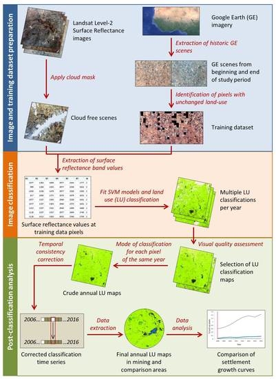
2.3.1. Image and Training Dataset Preparation

The Landsat Level-2 Pixel Quality Assessment band was used to create a cloud mask. The pixels that are interpreted as cloud or cloud shadow were removed from the original images using the “mask” function in the “raster” package in the statistical program R (Version 3.4.4, R Foundation for Statistical Computing, Vienna, Austria).
For the generation of a training dataset, suitable Google Earth scenes from the beginning and end of the study period were manually searched. By extracting imagery at different viewing heights, an optimal distance of 5.5 km was found to be ideal to still detect the different land uses while covering a large area. The Google Earth images were exported into ArcGIS (Version 10.5, ESRI, Redlands, CA, USA). In ArcGIS these scenes were then georeferenced to the Landsat scenes. Subsequently, a grid layer outlining the extents of the 30 m pixels of the Landsat scene was overlaid. Then, grid cells with stable land uses were identified for the following classes: water, grassland/agricultural land, forest, barren land, and built-up land, similar to Gong et al. (2015). Similar to the definition in other studies, a cell was assigned to a class if at least 50% of its area was composed of the respective land use class in the beginning and end of the study period [18,33,34].
Two different approaches were used to generate the training data. For the scenes covering the Bissa and Taparko mines, as well as their comparison areas, pixels from the whole scene were included as potential training data areas. For the other two scenes, which included the Essakane and Youga mines, the Google Earth images for generating the training data pixels were retrieved in the proximity of the areas of interest, i.e., within a 25 km buffer from the mining and comparison areas.

2.3.2. Image Classification

For the selection of the classification model, the performance of five different classifiers (random forest (RF), k-Nearest Neighbors, decision tree (KNN), support vector machine (SVM), linear discriminant analysis (LDA) and a classification and regression tree model (CART)) was tested on one randomly selected scene. Overall accuracy (OA) and the Kappa coefficient were determined by a 10-fold cross-validation with three resampling schemes. The highest accuracy was achieved by the SVM classifier (OA = 92.0%; K = 0.872) as compared to RF (OA = 88.4%; K = 0.799), KNN (91.9%; K = 0.870), LDA (OA = 84.6%; K = 0.754) and CART (OA = 79.5%; K = 0.677). Hence, the final classification method for predicting the land use classes consisted of fitting a separate SVM model (“svmRadial” function in “caret” R package) trained for each Landsat scene in the dataset. The algorithm was implemented using a radial kernel with hyperparameters set by default by the “caret” package. The Landsat surface reflectance band values at the training data pixel locations were extracted and used as input data for the learning of the hyperplane. Hence, 6 continuous input variables were used for Landsat 5 and 7 imagery; 7 variables for Landsat 8.

2.3.3. Post-Classification Processing

Three post-classification strategies were used to improve the accuracy and consistency of the classification. Firstly, the quality of each land use classification scene was assessed visually by the first author. Scenes with apparent misclassification due to haze, mist or other factors were excluded. Secondly, among all remaining scenes from the same year, the most commonly predicted land use class was taken at each pixel (i.e., mode) [35]. Random allocation to one of the classes was done in case of draws. Lastly, an adopted method from Chai et al. was applied to ensure temporal consistency [20]. It is based on the assumption that the conversion from built-up land to other land uses is highly unlikely and therefore assumed to be irreversible. Therefore, non-built-up pixels were reclassified as built-up if this was the assigned land use class in the two previous and the following year. Similarly, built-up pixels that appear isolated in a time series (i.e., pixels that were not built-up in the two years before and the following year) were reassigned the class of the previous year.

2.4. Accuracy Assessment

For each of the four scenes a separate validation dataset was created using Google Earth imagery. Reference data was only obtained in the study areas (i.e., within a 25 km buffer from the mine or comparison sites). In general, the same methodology as for the training dataset was used (see Section 2.3.1). However, due to the limited availability reference data in Google Earth covering the different land use classes, the accuracy assessment was only done for one year within the study period and merges the non-built-up classes into one “other” class.
The validation data was overlaid with the final classification result for the respective year to extract the OA, producer’s accuracy (PA), user’s accuracy (UA) and the Kappa coefficient.

2.5. Data Analysis

After excluding the mining area from the final classification, the number of built-up pixels within the mining and comparison buffers was extracted and the percentage of built-up pixels of the whole buffer zone calculated for each year. Annual settlement growth patterns were compared visually both between mining and comparison areas and between the years before and after mine opening. Based on previous studies and expert opinion on the likely impact radius of mining projects in remote settings, a 10 km and 25 km buffer was tested to determine the geographical extent of mining-related settlement growth [36].

3. Results

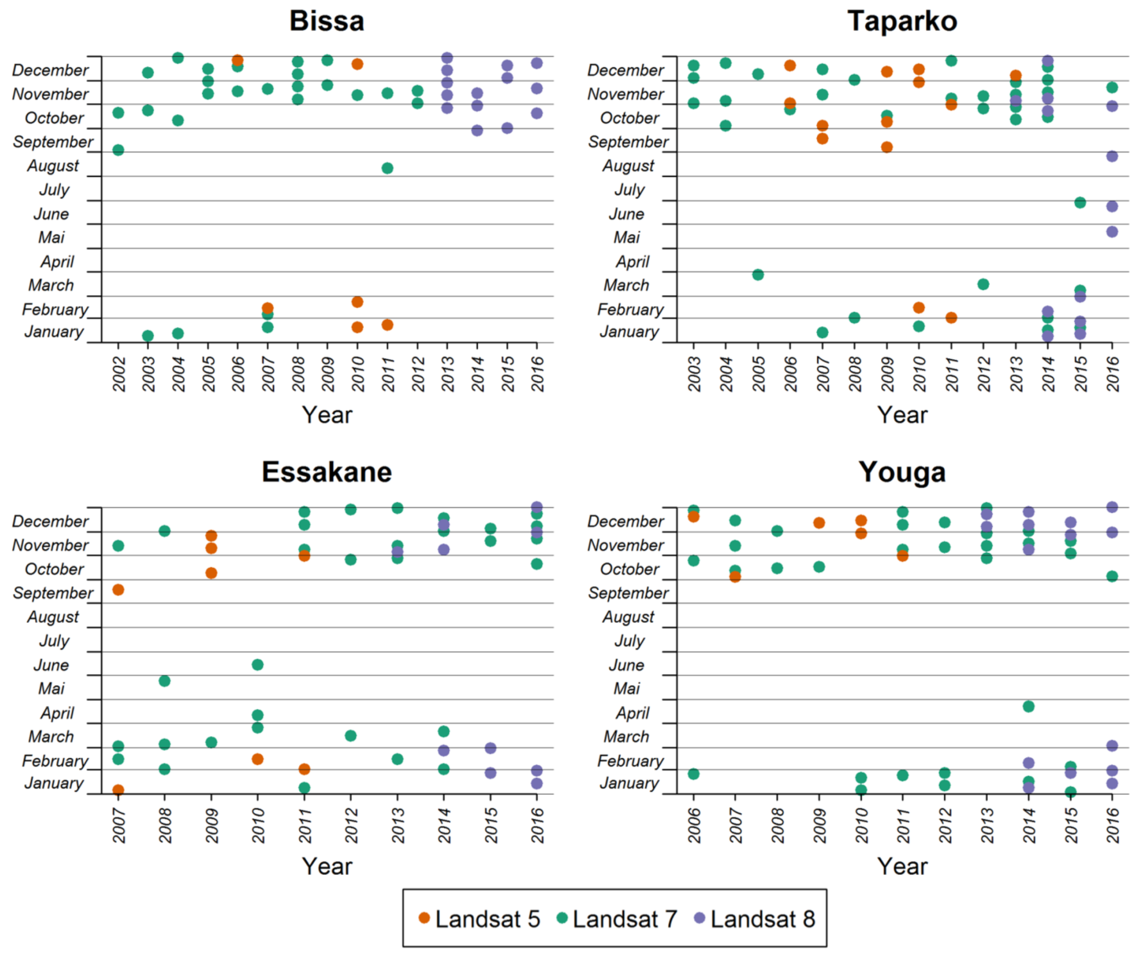
3.1. Availability of Landsat Satellite Imagery

Across sensors and study areas, 716 images with cloud cover below 10% were available (Table 1). The total number of downloaded images was 101, 428, and 187 from the Landsat 5, 7, and 8 missions, respectively. Until 2013, images from the Landsat 5 mission were available and the Landsat 8 satellite was launched in 2013. The Landsat 7 satellite provided images throughout the study period. However, since a failure in the Scan Line Corrector (SLC) in early 2003, the images show stripes of missing data.
Figure 3 depicts the capture dates of the retained satellite images that yielded high-quality land use maps using our approach. In total, 211 images were included for the post-classification steps (see Table 1). Of note, the vast majority of retained images were taken in the beginning (i.e., January and February) or the end (i.e., October–December) of the calendar year. These months coincide with the dry season in Burkina Faso.
For most years enough Landsat images could be retained. However, in a few instances only two useful images were available (e.g., in the Bissa area in 2012). In the case of disagreement between the two classifications, the modal value of the two initial land use classes was randomly assigned. Further, in some instances when only a few images were retained in the image stack, patches of missing data remained due to cloud coverage and gaps in SLC-off Landsat 7 scenes.

3.2. Availability of Historic Google Earth Imagery

More challenging than getting satellite imagery was to obtain Google Earth images to generate a training dataset valid for the entire study period. The availability of high-resolution imagery varied strongly depending on the location of the study area so that the start date of the study needed to be shifted. In general, older images were available over the capital Ouagadougou. In the more remote and rural areas, historic Google Earth imagery of sufficient resolution for determining land use was only available from around 2006/2007. Even in these instances, finding images covering all land use classes was cumbersome for that period. It was particularly challenging to delimit seasonal water bodies that partly or entirely dry out towards the end of the dry season.

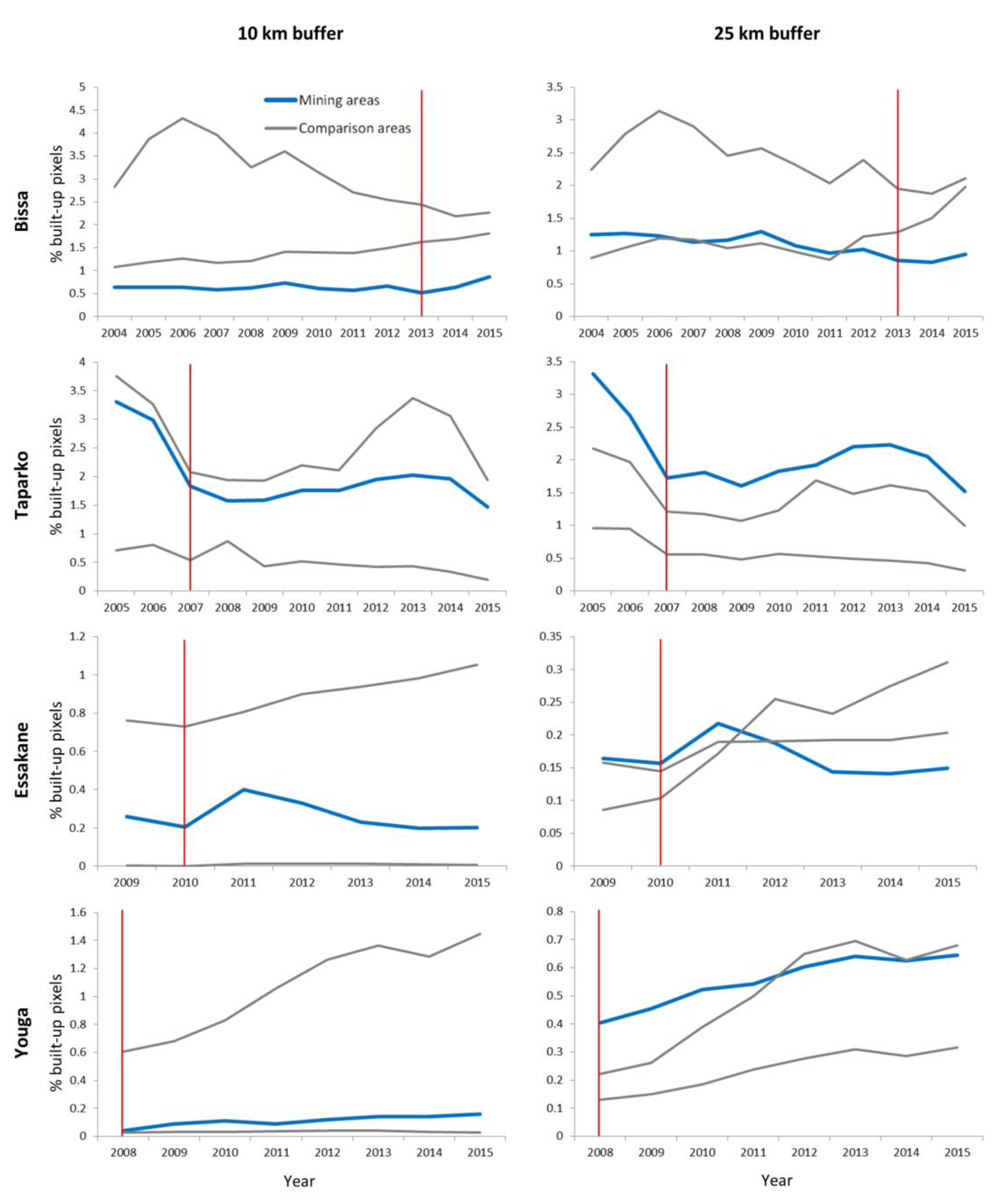
3.3. Settlement Growth in Mining and Non-Mining Areas

The percentage of built-up areas over time in the four mining areas and their comparison areas are depicted in Figure 4. Overall, differences in the variability of the growth curves were observed. In the areas where training data was obtained from anywhere within the satellite scene (i.e., Bissa and Taparko), a higher variability was observed. Indeed, there were a number of outliers in the classification in Bissa and Taparko leading to negative growth of settlements. For example, the raw classification for the Taparko scene in 2016 featured particularly few urban pixels and thereby leading to negative settlement growth in the previous year through the temporal consistency correction. Further, in the Bissa scene only two images were retained for 2009 and 2012 with extreme numbers of classified urban pixels. Visual inspection of the raw classification maps revealed that in these cases the misclassified urban pixels were mainly over barren and rocky ground. After application of the temporal consistency correction, the number of misclassified pixels could be reduced (see Figure 5).
Generating training data in the proximity of the areas of interest (i.e., Essakane and Youga) led to more stable results classification results over the years. Only in a few instances were negative growth years observed. In these areas a general urbanization trend, at different paces, was seen.
The growth curves showed different slopes both throughout the study period and across study areas. However, no clear pattern could be observed that could indicate strong in-migration to the studied mining areas. Although in some areas the settlements are at a greater distance from the mines, the growth patterns were similar in the different geographical extents.

3.4. Accuracy Assessment

Table 2 shows the result of the accuracy assessment. The OA for the different scenes were 86.4%, 58.5%, 80.3%, and 95.1% for Bissa, Taparko, Essakane, and Youga, respectively. Overall, there were large differences between the two approaches used for training data generation and between the study areas. The Kappa coefficient of the individual study areas ranged from as low as 0.176 to 0.902. Only in Youga was the classification sufficiently sensitive in detecting built-up pixels. In all scenes, only few non-built-up pixels were misclassified as built-up. Obtaining training data in the proximity of the study areas (approach 2) improved the accuracy substantially. However, in the Essakane scene only 30.4% of the built-up pixels in the reference dataset were correctly classified. Visual inspection of misclassified pixels revealed that most errors occurred in the less densely populated fringes of villages and at isolated clusters of buildings (see Figure 6).

4. Discussion

High-resolution Google Earth and 716 Landsat images were used to estimate annual settlement growth in rural mining areas in Burkina Faso. While the number of satellite images from Landsat was sufficient, finding adequate training data among historic Google Earth imagery was challenging. Indeed, in our study areas high-resolution imagery before 2006 was only available over larger urban areas. Still, using training data in proximity to the areas of interest reduced the inter-annual variability and resulted in higher classification accuracy. Overall accuracy of the four scenes ranged from 58.5% to 95.1%. These results show that with local training data and relatively humid environments the proposed methodology can yield stable and accurate estimates of settlement growth over time. However, due to the limited number of accurately classified study areas, no apparent differences in settlement growth patterns between mining and comparison areas were observed.
When comparing the growth curves of the predominantly rural areas selected for this paper with those of mainly urban areas reported in other publications, three patterns were observed: (i) the availability of Google Earth imagery influenced the classification accuracy; (ii) negative growth was observed in some study areas; and (iii) there is limited potential for additional post-classification correction approaches in our study setting. Each of these observations is discussed separately in the subsequent paragraphs.
Regarding the varying accuracy, it is noteworthy that the availability of historic high-resolution Google Earth imagery was limited. The available Google Earth scenes in the beginning and end of the study period had to be used as training data in order to meet the required sample size for fitting the SVM model [37]. When training data were located in cropped cloud areas or extents with remaining haze coverage, classification accuracy was low, leading to the exclusion of a substantial number of scenes during the visual quality assessment. Further, the accuracy assessment was limited to one extent in one year for each site because of the limited availability of Google Earth imagery. Still, the assessment indicates that for most scenes the number of undetected built-up pixels was substantially higher than in other studies [16,18], but also that the classification of the Youga scene provided very high accuracies. This scene differed in two aspects. Firstly, training data was obtained more closely to the area of interest, and secondly it is located further south in a tropical savanna climate. The lower accuracies in the other scenes may be caused by the similar spectral signatures of urban areas and natural bare surfaces (e.g., low normalized difference vegetation index (NDVI), an indicator for healthy vegetation) [29,34]. These similarities may be more pronounced in the semi-arid regions of northern Burkina Faso, where vegetation is sparse and the corrugated sheet roofs are often covered by a sand layer. Indeed, the vast majority of available cloud-free scenes used in this study were taken in the dry Harmattan season, characterized by dusty trade winds. Purposively selecting scenes shortly after the growing season might alleviate this problem.
A few other studies have also reported negative or absent settlement growth within their study period, although to a lesser degree [17,27]. Whether this was due to actual removal of buildings or misclassification errors is however not discussed. The higher variability found in the present study can partly be explained by the low percentage of built-up pixels in relatively small geographical areas. Hence, misclassification of, e.g., a patch of rocky ground into the built-up class will lead to a significant spike in the number of urban pixels in that year. Further, the absence of accelerated growth patterns in mining areas may also be due to a densification of housing within the existing settlement extents, which is difficult to detect at 30 m pixel size.
Regarding post-classification approaches, other studies observed that more robust results were obtained when incorporating spatial consistency checks, in addition to the temporal consistency correction as applied in this study [33,38]. This approach includes a calculation of the probability of a pixel to be urban as a function of the surrounding pixels. Although this may reduce the “salt and pepper” effect in scattered sparsely populated areas in rural sub-Saharan Africa where building clusters only cover a few pixels, this may lead to an underestimation of the built-up areas.
The strength of the method used in this study is the reliance on globally and freely available data and its relatively straight-forward workflow relying on few image pre-processing steps. This could make it useful for researchers and public institutions with limited technical expertise to track settlement changes in areas where reliable and up-to-date population data is scarce. In these cases, the Google Earth training data could be complemented with additional ground-truth points from field observations.
As the repositories are continuously built up, Landsat and high-resolution Google Earth imagery will become increasingly available for longer periods allowing for long-term tracking of population growth remote areas. Additionally, other imagery from more recently launched satellite missions could be incorporated in the workflow. For example, the Sentinel-2 satellites provide freely available imagery at a 10–60 m resolution on a nearly global coverage since 2015 [39]. While this timeframe was not sufficient for the present study, it could serve as a good baseline for future endeavors for multi-annual land use classifications [27,39]. Still, the increased resolution could reduce the problem of pixels featuring multiple land use classes.
Future studies should also investigate the performance of the approach in remote areas in other climatic zones, potentially incorporating other spectral indices, such as NDVI or natural built-up index (NDBI). Additionally, in order to determine the magnitude of mining-related population growth, more long-term studies covering a higher number of mining areas are needed.

5. Conclusions

The applicability of the proposed methodology depends on the availability of historic Google Earth imagery and climatic factors. High accuracy in annual estimation of rural settlement growth was achieved when two conditions were met: (i) training data were available in proximity to the areas of interest; and (ii) the setting was located in the relatively humid areas in southern Burkina Faso. Hence, in humid climate zones and locations with high quality satellite imagery in proximity to the area of interest, the developed methodology can be readily applied for further investigating the impacts of mining and other large infrastructure projects on population growth in remote locations. Indeed, the increasing availability of long-term high-resolution satellite imagery through Google Earth, but also new data sources such as imagery from the Sentinel missions, will further increase the potential applications of the developed methodology.

Author Contributions

Conceptualization, D.D., K.d.H. and M.S.W.; methodology, D.D., A.F., K.d.H. and M.S.W.; formal analysis, D.D.; writing—original draft preparation, D.D.; writing—review and editing, A.F., K.d.H. and M.S.W.; supervision, A.F., K.d.H. and M.S.W. All authors have read and agreed to the published version of the manuscript.

Funding

This work is part of the r4d program (www.r4d.ch), which is a joint funding initiative by the Swiss Agency for Development and Cooperation (SDC) and the Swiss National Science Foundation (SNSF) [grant number 169461].

Acknowledgments

The authors thank the technical guidance from Andreas Wicki from the Department of Environmental Sciences of the University of Basel.

Conflicts of Interest

The authors declare no conflict of interest. The funders had no role in the design of the study; in the collection, analyses, or interpretation of data; in the writing of the manuscript, or in the decision to publish the results.

References

  1. Jackson, R.T. Migration to two mines in Laos. Sustain. Dev. 2018, 26, 471–480. [Google Scholar] [CrossRef]
  2. Nyame, F.K.; Andrew Grant, J.; Yakovleva, N. Perspectives on migration patterns in Ghana’s mining industry. Resour. Policy 2009, 34, 6–11. [Google Scholar] [CrossRef]
  3. IFC. Projects and People: A Handbook for Addressing Project-Induced In-Migration; International Finance Corporation: Washington, DC, USA, 2009. [Google Scholar]
  4. Loayza, F.; Franco, I.; Quezada, F.; Alvarado, M.; Castillo, J.; Sanchez, J.M.; Kunze, V.; Araya, R.; Pasco-Font, A.; Diez Hurtado, A.; et al. Large Mines and the Community: Socioeconomic and Environmental Effects in Latin America, Canada, and Spain; McMahon, G., Remy, F., Eds.; World Bank: Washington, DC, USA, 2001; ISBN 978-0-88936-949-8. [Google Scholar]
  5. Winkler, M.S.; Krieger, G.R.; Divall, M.J.; Singer, B.H.; Utzinger, J. Health impact assessment of industrial development projects: A spatio-temporal visualization. Geospat. Health 2012, 6, 299–301. [Google Scholar] [CrossRef] [Green Version]
  6. Petkova, V.; Lockie, S.; Rolfe, J.; Ivanova, G. Mining Developments and Social Impacts on Communities: Bowen Basin Case Studies. Rural Soc. 2009, 19, 211–228. [Google Scholar] [CrossRef]
  7. Stevens, F.R.; Gaughan, A.E.; Nieves, J.J.; King, A.; Sorichetta, A.; Linard, C.; Tatem, A.J. Comparisons of two global built area land cover datasets in methods to disaggregate human population in eleven countries from the global South. Int. J. Digit. Earth 2020, 13, 78–100. [Google Scholar] [CrossRef]
  8. Wardrop, N.A.; Jochem, W.C.; Bird, T.J.; Chamberlain, H.R.; Clarke, D.; Kerr, D.; Bengtsson, L.; Juran, S.; Seaman, V.; Tatem, A.J. Spatially disaggregated population estimates in the absence of national population and housing census data. Proc. Natl. Acad. Sci. USA 2018, 115, 3529–3537. [Google Scholar] [CrossRef] [Green Version]
  9. Tatem, A.J. Mapping the denominator: Spatial demography in the measurement of progress. Int. Health 2014, 6, 153–155. [Google Scholar] [CrossRef] [Green Version]
  10. United Nations. Principles and Recommendations for Population and Housing Censuses: 2020 Round; United Nations, Ed.; Economic & Social Affairs; Revision 3; United Nations: New York, NY, USA, 2017; ISBN 978-92-1-161597-5. [Google Scholar]
  11. Acheampong, R.A.; Agyemang, F.S.K.; Abdul-Fatawu, M. Quantifying the spatio-temporal patterns of settlement growth in a metropolitan region of Ghana. GeoJournal 2017, 82, 823–840. [Google Scholar] [CrossRef] [Green Version]
  12. Zhao, Y.; Feng, D.; Yu, L.; Cheng, Y.; Zhang, M.; Liu, X.; Xu, Y.; Fang, L.; Zhu, Z.; Gong, P. Long-Term Land Cover Dynamics (1986–2016) of Northeast China Derived from a Multi-Temporal Landsat Archive. Remote Sens. 2019, 11, 599. [Google Scholar] [CrossRef] [Green Version]
  13. Wulder, M.A.; Masek, J.G.; Cohen, W.B.; Loveland, T.R.; Woodcock, C.E. Opening the archive: How free data has enabled the science and monitoring promise of Landsat. Remote Sens. Environ. 2012, 122, 2–10. [Google Scholar] [CrossRef]
  14. Woodcock, C.E.; Allen, R.; Anderson, M.; Belward, A.; Bindschadler, R.; Cohen, W.; Gao, F.; Goward, S.N.; Helder, D.; Helmer, E.; et al. Free Access to Landsat Imagery. Science 2008, 320, 1011. [Google Scholar] [CrossRef] [PubMed]
  15. Phiri, D.; Morgenroth, J. Developments in Landsat Land Cover Classification Methods: A Review. Remote Sens. 2017, 9, 967. [Google Scholar] [CrossRef] [Green Version]
  16. Gong, P.; Li, X.; Zhang, W. 40-Year (1978–2017) human settlement changes in China reflected by impervious surfaces from satellite remote sensing. Sci. Bull. 2019, 64, 756–763. [Google Scholar] [CrossRef] [Green Version]
  17. Sexton, J.O.; Song, X.-P.; Huang, C.; Channan, S.; Baker, M.E.; Townshend, J.R. Urban growth of the Washington, D.C.–Baltimore, MD metropolitan region from 1984 to 2010 by annual, Landsat-based estimates of impervious cover. Remote Sens. Environ. 2013, 129, 42–53. [Google Scholar] [CrossRef]
  18. Schneider, A. Monitoring land cover change in urban and peri-urban areas using dense time stacks of Landsat satellite data and a data mining approach. Remote Sens. Environ. 2012, 124, 689–704. [Google Scholar] [CrossRef]
  19. Hu, T.; Yang, J.; Li, X.; Gong, P. Mapping Urban Land Use by Using Landsat Images and Open Social Data. Remote Sens. 2016, 8, 151. [Google Scholar] [CrossRef]
  20. Chai, B.; Li, P. Annual Urban Expansion Extraction and Spatio-Temporal Analysis Using Landsat Time Series Data: A Case Study of Tianjin, China. IEEE J. Sel. Top. Appl. Earth Obs. Remote Sens. 2018, 11, 2644–2656. [Google Scholar] [CrossRef]
  21. Gong, P.; Wang, J.; Yu, L.; Zhao, Y.; Zhao, Y.; Liang, L.; Niu, Z.; Huang, X.; Fu, H.; Liu, S.; et al. Finer resolution observation and monitoring of global land cover: First mapping results with Landsat TM and ETM+ data. Int. J. Remote Sens. 2013, 34, 2607–2654. [Google Scholar] [CrossRef] [Green Version]
  22. Taubenböck, H.; Esch, T.; Felbier, A.; Wiesner, M.; Roth, A.; Dech, S. Monitoring urbanization in mega cities from space. Remote Sens. Environ. 2012, 117, 162–176. [Google Scholar] [CrossRef]
  23. Ayele, G.T.; Tebeje, A.K.; Demissie, S.S.; Belete, M.A.; Jemberrie, M.A.; Teshome, W.M.; Mengistu, D.T.; Teshale, E.Z. Time Series Land Cover Mapping and Change Detection Analysis Using Geographic Information System and Remote Sensing, Northern Ethiopia. Air Soil Water Res. 2018, 11, 1–18. [Google Scholar] [CrossRef] [Green Version]
  24. Wohlfart, C.; Mack, B.; Liu, G.; Kuenzer, C. Multi-faceted land cover and land use change analyses in the Yellow River Basin based on dense Landsat time series: Exemplary analysis in mining, agriculture, forest, and urban areas. Appl. Geogr. 2017, 85, 73–88. [Google Scholar] [CrossRef]
  25. Reynolds, R.; Liang, L.; Li, X.; Dennis, J. Monitoring Annual Urban Changes in a Rapidly Growing Portion of Northwest Arkansas with a 20-Year Landsat Record. Remote Sens. 2017, 9, 71. [Google Scholar] [CrossRef] [Green Version]
  26. Schneider, A.; Mertes, C.M. Expansion and growth in Chinese cities, 1978–2010. Environ. Res. Lett. 2014, 9, 024008. [Google Scholar] [CrossRef]
  27. Schug, F.; Okujeni, A.; Hauer, J.; Hostert, P.; Nielsen, J.Ø.; van der Linden, S. Mapping patterns of urban development in Ouagadougou, Burkina Faso, using machine learning regression modeling with bi-seasonal Landsat time series. Remote Sens. Environ. 2018, 210, 217–228. [Google Scholar] [CrossRef]
  28. Qin, Y.; Xiao, X.; Dong, J.; Chen, B.; Liu, F.; Zhang, G.; Zhang, Y.; Wang, J.; Wu, X. Quantifying annual changes in built-up area in complex urban-rural landscapes from analyses of PALSAR and Landsat images. ISPRS J. Photogramm. Remote Sens. 2017, 124, 89–105. [Google Scholar] [CrossRef] [Green Version]
  29. Li, X.; Zhou, Y.; Zhu, Z.; Liang, L.; Yu, B.; Cao, W. Mapping annual urban dynamics (1985–2015) using time series of Landsat data. Remote Sens. Environ. 2018, 216, 674–683. [Google Scholar] [CrossRef]
  30. Farnham, A.; Cossa, H.; Dietler, D.; Engebretsen, R.; Leuenberger, A.; Lyatuu, I.; Nimako, B.; Zabre, H.R.; Brugger, F.; Winkler, M.S. A mixed methods approach for investigating health impacts of natural resource extraction projects in Burkina Faso, Ghana, Mozambique, and Tanzania: A study protocol. JMIR Res. Protoc. 2019. under review. [Google Scholar]
  31. Winkler, M.S.; Adongo, P.B.; Binka, F.; Brugger, F.; Diagbouga, S.; Macete, E.; Munguambe, K.; Okumu, F. Health impact assessment for promoting sustainable development: The HIA4SD project. Impact Assess. Proj. Apprais. 2020, in press. [Google Scholar] [CrossRef] [Green Version]
  32. INSD. Recensement Génélral de la Population et de L’habitation au Burkina Faso en 2006; Institut National de la Statistique et de la Démographie: Ouaga, Burkina Faso, 2006.
  33. Li, X.; Gong, P.; Liang, L. A 30-year (1984–2013) record of annual urban dynamics of Beijing City derived from Landsat data. Remote Sens. Environ. 2015, 166, 78–90. [Google Scholar] [CrossRef]
  34. Li, X.; Gong, P. An “exclusion-inclusion” framework for extracting human settlements in rapidly developing regions of China from Landsat images. Remote Sens. Environ. 2016, 186, 286–296. [Google Scholar] [CrossRef]
  35. Wicki, A.; Parlow, E. Attribution of local climate zones using a multitemporal land use/land cover classification scheme. J. Appl. Remote Sens. 2017, 11, 026001. [Google Scholar] [CrossRef] [Green Version]
  36. Punam, C.-P.; Dabalen, A.L.; Kotsadam, A.; Aly, S.; Tolonen, A.K. The Local Socioeconomic Effects of Gold Mining: Evidence from Ghana; World Bank Group: Washington, DC, USA, 2015. [Google Scholar]
  37. Vanniel, T.; Mcvicar, T.; Datt, B. On the relationship between training sample size and data dimensionality: Monte Carlo analysis of broadband multi-temporal classification. Remote Sens. Environ. 2005, 98, 468–480. [Google Scholar] [CrossRef]
  38. Shi, L.; Ling, F.; Ge, Y.; Foody, G.; Li, X.; Wang, L.; Zhang, Y.; Du, Y. Impervious Surface Change Mapping with an Uncertainty-Based Spatial-Temporal Consistency Model: A Case Study in Wuhan City Using Landsat Time-Series Datasets from 1987 to 2016. Remote Sens. 2017, 9, 1148. [Google Scholar] [CrossRef] [Green Version]
  39. Wulder, M.A.; Hilker, T.; White, J.C.; Coops, N.C.; Masek, J.G.; Pflugmacher, D.; Crevier, Y. Virtual constellations for global terrestrial monitoring. Remote Sens. Environ. 2015, 170, 62–76. [Google Scholar] [CrossRef] [Green Version]
Figure 1. Location of gold mining areas included in this study.
Remotesensing 12 00235 g001
Figure 2. Data sources and methodological flowchart. GE: Google Earth. SVM: support vector machine. LU: land use.
Remotesensing 12 00235 g002
Figure 3. Capture dates of images retained after the visual quality assessment for each study site and year.
Remotesensing 12 00235 g003
Figure 4. Comparison of the percentage of built-up pixels over time. Blue lines depict settlement growth in mining areas over time. Gray lines show settlement growth in comparable nearby districts within a 10 km (left panels) and 25 km (right panels) radius. Red vertical bars indicate the opening year of the mine.
Remotesensing 12 00235 g004
Figure 5. Visualization of the impact of the temporal consistency correction. Crude growth curves are depicted with dashed lines; corrected growth curves with solid lines. This example shows the trends in the 10 km buffer around the Bissa mine (blue line) and its comparison areas (grey lines).
Remotesensing 12 00235 g005
Figure 6. Examples of correctly (green) and incorrectly (red) classified pixels (30 × 30 m). (A) Extent near the Bissa mine with high accuracy. (B) Undetected urban pixels at the fringes of a settlement in Taparko area.
Remotesensing 12 00235 g006
Table 1. Available Landsat images with <10% cloud cover by study area and Landsat mission. Numbers in parentheses indicate the number of retained images after the visual quality assessment of the initial land use classification.
Landsat MissionBissaTaparkoEssakaneYougaTotal
Landsat 525 (6)28 (13)27 (8)21 (6)101 (33)
Landsat 7133 (27)117 (35)95 (32)83 (32)428 (126)
Landsat 846 (14)48 (13)53 (10)40 (15)187 (52)
Total204 (47)193 (61)175 (50)144 (53)716 (211)
Table 2. Accuracy assessment by training data generation approach and study area. Approach 1 refers to obtaining training data within the whole scene. In approach 2 training data was only generated from the proximity of the study areas. Overall accuracy (OA), producer’s accuracy (PA), user’s accuracy (UA) and the Kappa coefficient are reported.
Approach 1Classification Approach 2Classification
ReferenceBuilt-upOtherPAReferenceBuilt-upOtherPA
Built-up13019739.8%Built-up4389981.6%
Other2746294.5%Other370399.6%
UA82.8%70.1% UA95.0%87.7%
OA = 72.5%OA = 91.8%
Kappa = 0.375Kappa = 0.829
BissaClassification TaparkoClassification
ReferenceBuilt-upOtherPAReferenceBuilt-upOtherPA
Built-up705257.4%Built-up6014529.3%
Other428598.6%Other2317788.5%
UA94.6%84.6% UA72.3%55.0%
OA = 86.4%OA = 58.5%
Kappa = 0.632Kappa = 0.176
EssakaneClassificationPAYougaClassificationPA
ReferenceBuilt-upOther ReferenceBuilt-upOther
Built-up245530.4%Built-up4144490.4%
Other0200100%Other350399.4%
UA100%78.4% UA99.3%92.0%
OA = 80.3%OA = 95.1%
Kappa = 0.385Kappa = 0.902

