1. Introduction
Over recent decades, the number of openly available geographic data sets has tremendously increased along with their use in policy making, environmental monitoring, hazard prevention and scientific studies. It is of paramount importance that their quality is rigorously evaluated to inform users about their limitations and to limit contradicting results. Good practices in accuracy assessment include recommendations about (1) the sampling design that determine how many sampling units should be collected along with their locations; (2) the response design that defines the protocol for labeling each sampling unit; and (3) a rigorous estimation of accuracy using specific metrics [
1,
2,
3,
4,
5]. A statistically rigorous assessment is thus a combination of a probability sampling design, appropriate accuracy estimators, and a response design chosen in accordance with features of the mapping and classification process.
Uncertainties linked to the sampling design and variance of the estimators are usually well quantified, but validation methods typically assume that reference data are error-free. In fact, the process of determining the so-called “ground truth” is seldom discussed in the literature and is often considered a straightforward—yet costly—task. Nonetheless, generating authoritative reference data sets remains a major challenge in accuracy assessment and it merits greater consideration in accuracy assessment [
6]. Errors can indeed alter the process of generating reference data and even a small amount of errors can propagate and significantly impact the accuracy assessment [
7,
8,
9]. There is thus a need for new methods that offer better control over the quality of reference data.
Practical constraints, such as poor accessibility to the sample locations on the ground, often affect the implementation of an ideal accuracy assessment protocol. For instance, this prompted Stehman [
4] to propose criteria for quality and statistical rigor while taking, at the same time, practical utility (accessibility and reduced costs) into account. Another alternative is to replace ground observations with photo-interpreted very high-resolution images. Photo-interpretation by a group of experts with regional knowledge is often seen as the gold standard for reference data collection when dealing with large-area thematic products. However, photo-interpretation is not perfect—it typically reaches 80% accuracy—and it varies considerably among operators with accuracy levels ranging from 11% up to 100% [
10]. Thematic errors (
e) affecting photo-interpreted samples can be divided in three categories: vigilance, systematic, and estimation errors:
Vigilance errors, i.e., loss of performance after performing the same monotonous task over a long period, has been highlighted for a wide range of visual interpretation tasks [
11]. Attitude, either optimistic or pessimistic, may determine how an operator will respond to training for vigilance [
12]. Drops of vigilance, which are difficult to predict and manage for an individual interpreter, can be reduced by relying on more than one operator [
13] either with consensual labeling or automated cross-validation.
Systematic errors (
) occur when a photo-interpreter is incorrectly reading images. Reading of images and maps belongs to cartographic and visual literacy [
14], a skill that changes over time and can be improved with the development of geospatial thinking. Image interpretation is a process that combines perception and cognition, both of which tend to facilitate identification (the cognitive task of identifying a pattern) and signification (the assignment of a meaning to a particular pattern [
15,
16]). The types of insight derived from imagery are strongly influenced by the interpreter’s expertise. Experts bring specialized knowledge, highly attuned perceptual skills and flexible reasoning abilities that novices lack [
17]. There is however not always a strong relationship between the field work experience of operators and their photo-interpretation accuracy [
18]. This might be explained by the dissimilarities between, on one side, air- and spaceborne images and, on the other side, panoramic images in at least three important aspects: (1) the portrayal of features from a downwards—often unfamiliar—perspective; (2) the use of wavelengths outside the visual portion of the spectrum; and (3) the depiction of the Earth’s surface at unfamiliar scales and resolutions [
19]. The most capable interpreters have keen powers of observation, coupled with imagination and a great deal of patience [
19]. Another individual factor potentially influencing image interpretation accuracy is search strategy. Compared to random search, training in systematic inspection caused higher performance [
20]. Maruff et al. [
21] have suggested that behavioral goals constrain the selection of visual information more than the physical characteristics of the information. This suggests that photo-interpreters with a search strategy based on previous experiences would be more successful at extracting relevant information than someone randomly searching for this information. Geographers would therefore be more successful than non-geographers during a single categorization round of aerial photos [
22]. Accordingly, crowdsourcing (i.e., when photo-interpreters are replaced by volunteers) is particularly prone to errors as it is open to anyone, regardless of the level of expertise of the volunteers. Systematic errors can thus largely be avoided by providing training to photo-interpreters, by selecting operators with local knowledge and by relying on multiple contributors [
13].
Estimation errors (
) arise when the class proportions within sampling units are imprecise even when all labels related to the sampling units are correct. These errors stem from three main factors: the number of sub-samples to label per sampling unit, the landscape structure, and the classification system. Imprecise estimates of the proportion of different classifiers for mixed or transitional classes reportedly account for most disagreements among photo-interpreters [
23]. It has also been shown that the accuracy of the labeling as well as the accuracy of the image-based classification generally decrease when the sub-pixel heterogeneity increases [
24]. Contrary to the systematic and vigilance errors, there is currently no mechanism to control estimation errors. Therefore, even when best practices in quality control are implemented (i.e.,
and
), uncertainties in the photo-interpreted labels remain due to estimation errors. If left unchecked, these estimation errors can bias reference data and subsequent accuracy assessments for they are intrinsically linked to the complexity of the sub-pixel landscape structure. Here, we propose that estimation errors need to be managed in the response design.
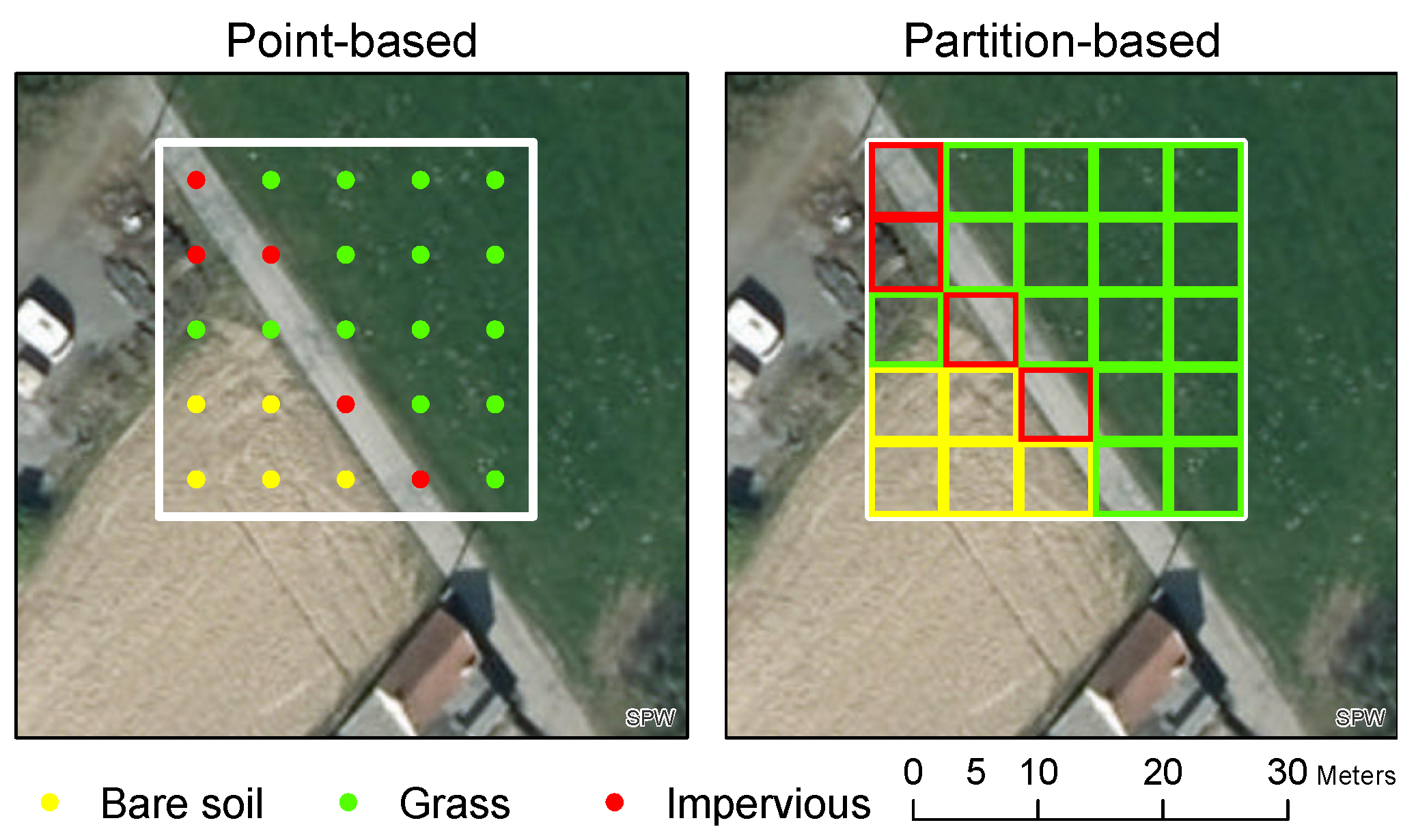
The objective of this paper is to untangle the intricate interplay between classification systems, response designs and landscape fragmentation with regards to the estimation errors. Specifically, we (1) quantify the impact of imprecise estimation of land-cover proportions on the accuracy of reference data; and (2) propose a response design that optimizes the labeling effort. We particularly focused on two aspects of response designs for binary and multiclass majority classification systems: their structure (point-based vs. partition-based designs) and the labeling effort (the number of sub-samples to be labeled per sampling unit). Because the three components of the errors (Equation (
1)) are strongly intertwined in real case studies, we relied on synthetic ground truth data which gave full control over the sampling strategy and allowed us to isolate estimation errors. Synthetic ground truth is indeed necessary to ensure that the actual properties of the data were known and to exclude effects due to other sources of ground reference data error [
25,
26,
27]. Our main contributions can be summarized as follows:
We provide an in-depth review of the different types of response designs and their applications;
We analyze the performance of response designs for different types of classification systems;
We generalize case-specific results using indices of landscape composition;
We optimize the sampling effort with adaptive response designs that leverage the confidence intervals of the estimated proportions.
4. Methods
We sought to answer the following questions:
What is the accuracy of point-based and partition-based response designs for different number of sub-samples in a realistic case study?
How can the accuracy of response designs be predicted based on landscape structure indices?
How to optimize the number of sub-samples per sampling unit?
We addressed these questions in three successive steps for the four classification systems described in
Section 3.2. First, the accuracy of the various response designs was compared with simulated sampling across the study site (
Section 4.1). Second, we generalized the relationship between the error rate and the underlying landscape of sampling units (
Section 4.2). We finally proposed a method that iteratively adds sub-samples to label until the estimated class proportions driving the labeling process reach the desired confidence level (
Section 4.3).
This optimization method is formulated for point-based designs only, as theoretical confidence intervals are not available for partition-based designs and labels cannot be reused when the number of partitions is increased. In fact, optimizing the partition-based designs depends on the ability of the operator to decide the appropriate number of sub-samples. As we assumed perfect operators throughout this paper, the question of optimizing partition-based designs falls beyond the scope of this paper. Nonetheless, the impact of photo-interpretation errors on the response design is discussed in
Section 6.
4.1. Accuracy of Point-Based and Partition-Based Response Designs
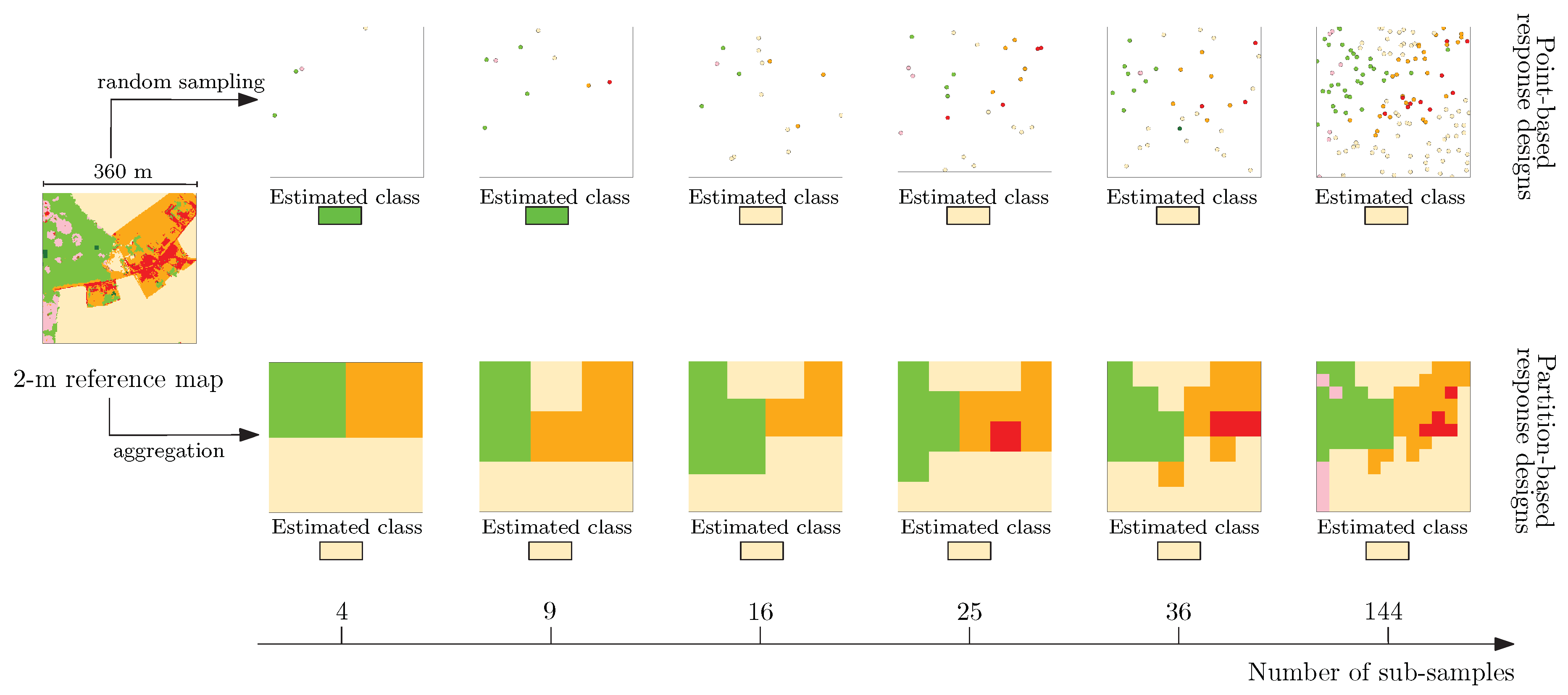
Our approach to empirically quantify the accuracy of response designs was based on a Monte Carlo framework. For every sampling unit, we repeatedly estimated the class proportions of ground truth for a range of sub-sampling efforts. The labels of the randomly simulated response designs were then assigned using the decision rules of the four classification systems. The same decision rules were applied on the true proportions (i.e., computed from the 2-m reference map) to derive the true label. For each iteration, the error rate was computed by dividing the number of disagreements between the true and the simulated labels of the sampling units, with
For the point-based response designs, the sub-sample selection was repeated 36 times. Sub-samples were selected by simple probabilistic sampling of the 2-m pixels located inside each sampling unit.
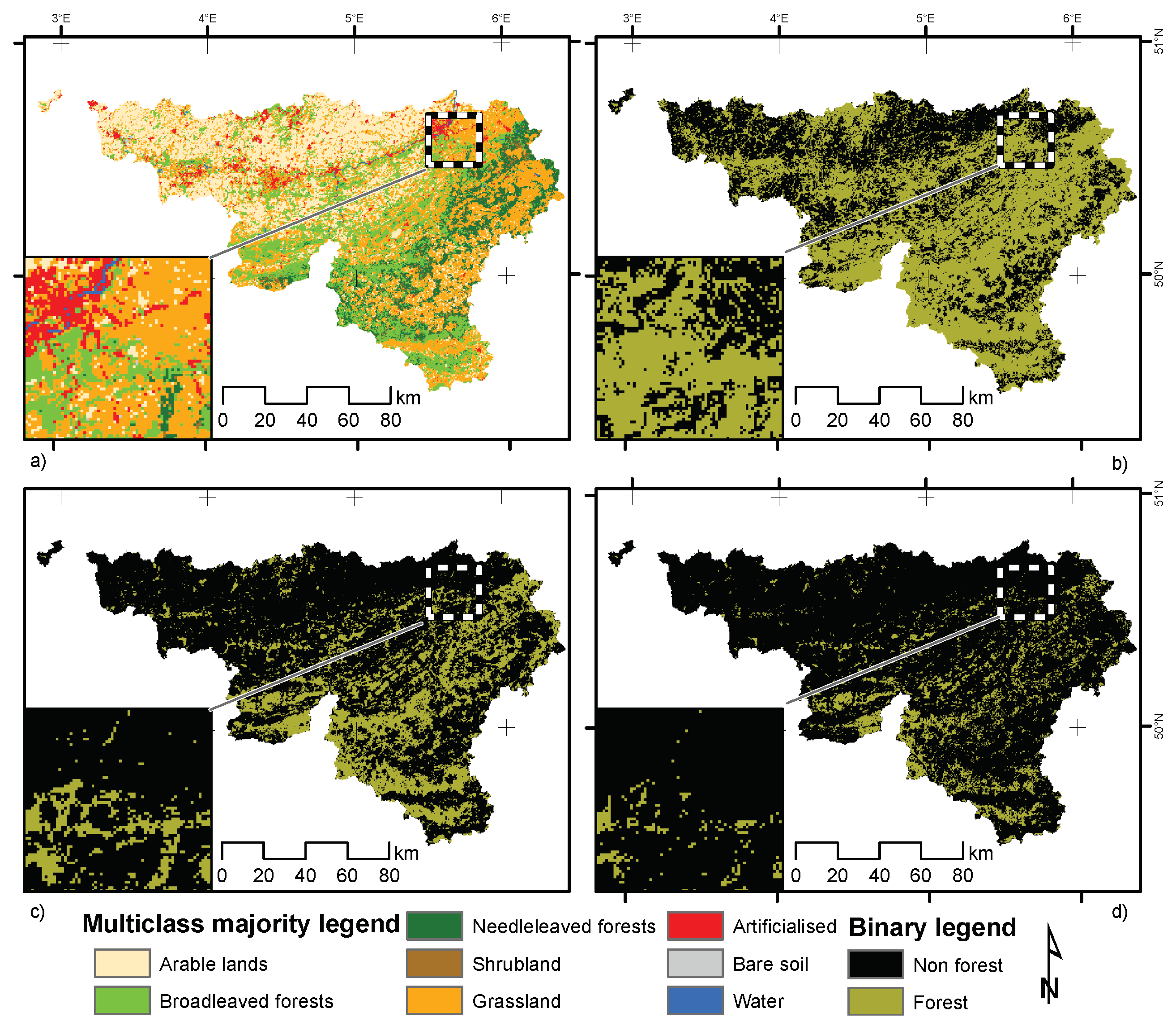
For partition-based response designs, the 36 realizations were generated by shifting the origin of the grid by six multiples of 11 pixels (22, 33, 44, 55, 66, 77) in both the x and y directions (sampling units that are not completely inside the study area were discarded). Spatial resampling of the 2-m reference map was performed at intermediate spatial resolutions of 180, 120, 90, 72, 60, 36 and 30 m, which correspond to a partitioning in 4, 9, 16, 25, 36, 100 and 144 squares, respectively. These resolutions were constrained by the availability of integer divisors of 180. For the sake of comparison, the same numbers of sub-samples were used for the point-based approach. In the TTM case, the proportion of the forest class was computed within every intermediate resolution pixel, which were then labeled as forest or non-forest according to the threshold value. Those pixels were then resampled at the spatial resolution of 360 m with a majority rule to select the final label. In the MTT case, the forest label was assigned to each sub-sample where forest was the majority class. The proportion of forest pixels was then computed for each 360 m pixel and the final forest/non-forest label was assigned based on the selected threshold. For the majority classification system, the majority class was first identified for each sub-sample, then the majority of the sub-sample labels was assigned to the sampling unit.
4.2. Impact of Landscape Fragmentation
We sought to evidence the link between landscape structure and response design to predict the response design accuracy in other landscapes where prior structure knowledge is available. We therefore selected two landscape metrics, one per type of classification system, which can be easily computed for any areal sampling unit and any scale.
For binary classification systems, we characterized landscapes by reporting the proportion of our main class within each sampling unit. Because there is only one degree of freedom with two classes, the choice of the main class does not influence the reasoning, hence the forest class was arbitrarily selected, with:
where
is the area of forest (more precisely in this case, tree crown cover) inside the sampling unit, and
is the area of the sampling unit.
For multiclass classification systems, we opted for the Equivalent Reference Probability (
) [
51]. Rooted in information theory, the equivalent reference probability is particularly interesting because it accounts for the full set of probabilities and remains consistent with the maximum probability, unlike entropy. Given
the vector of the class proportions in the landscape,
k the number of classes and
the index of the dominant class, the equivalent reference probability is
where
is the expected difference of information as described in equation:
with
, the proportion of the majority class. Class purity and
were computed for each sampling unit based on the true proportions.
Average error rates of the response designs were estimated for the full range of possible
and
values with a step of
. For visualization purposes, the error rate was smoothed by fitting local regressions LOESS [
52].
4.3. Local Optimization of the Number of Sub-Samples
When collecting validation data, the structure of the landscapes covered by the sample units is generally unknown, so that the optimal number of sub-sampling units cannot be estimated a priori from relationships between accuracy and landscape fragmentation. However, thanks to the interactivity of the Web 2.0, online validation platforms can be tailored to compute and update class proportion estimates as soon as sub-samples are labeled by photo-interpreters. This part of the study aimed to optimize the number of sub-samples needed for reaching a certain level of accuracy, resulting in an optimal response design that minimizes costs and/or time constraints. We propose to define an optimal number of sub-samples for each sampling unit based on the confidence intervals of the estimated sub-sample class proportions. Here, the confidence levels were set to 99.9% to illustrate the stringent requirements of building authoritative reference data sets, and to 90% to illustrate the required effort for collecting reference data under constrained conditions.
In practice, the local optimization process consisted of randomly selecting an initial set of nine sub-samples and assessing the corresponding confidence level. Sub-samples were then added one at a time until the confidence on the estimated proportions reached the desired confidence. For binary classification systems, the confidence interval (for a given confidence level) around the estimated proportion must not include the threshold value that divides the study area in the two binary classes. For the multiclass majority classification system, the confidence interval around the estimated proportions of the majority class must not include the estimated proportion of the second most frequent class.
For binary classification systems, a given sampling unit is correctly labeled if the estimated proportion is on the same side of the threshold value as the true proportion. In practice, the proportion of the sampled area is unknown. However, the probability of assigning the correct label can be estimated based on the estimated value of the binomial distribution.
The confidence interval around estimated class proportions or accuracy indices is usually estimated using a Normal approximation
where
is the confidence interval lower bound,
is the confidence interval upper bound,
n is the number of sub-sampling units,
m is the number of points belonging to the class label selected by the decision rule, z is a percentile from the standard normal distribution and
is the percent chance of making a Type I error (so that
is the confidence level).
However, the two main hypotheses of the Normal approximation are not respected in our incremental case: the number of points is small and proportions close or equal to 1 (pure pixels) are likely to be observed. The Clopper-Pearson exact confidence interval (CI) was therefore used instead of the Normal approximation [
53], with
where
is the confidence interval lower bound,
is the confidence interval upper bound,
n is the number of sub-sampling units,
m is the number of points belonging to the majority class,
is the percent chance of making a Type I error, and
is the confidence level. Those parameters are taken by the BetaInv function, which computes the inverse of the beta cumulative distribution function.
Exact confidence intervals are not available for multinomial cases. Several approximations have been proposed [
54,
55,
56]. Simultaneous confidence interval estimates from Goodman [
56] were selected because preliminary tests revealed that in a binomial case, it provides a closer match to the Clopper-Pearson interval than other alternatives. For a multinomial distribution
, Goodman’s simultaneous confidence interval for the
class is given by
where
is the proportion of class
i,
n is the total number of samples and
, the
quantile of the chi-square distribution with one degree of freedom.
In some cases, e.g., where the observed class proportion is equal to the arbitrary threshold in a binary classification or when several classes have the same proportion in the case of majority rule, the number of points to meet the required confidence could grow infinitely. Therefore, the maximum number of points was arbitrarily set to 144. This process was repeated 25 times to compare the theoretical confidence levels with the observed accuracy and to estimate the average number of sub-samples needed for each sampled area.
5. Results
5.1. Impact of Response Design and Sampling Effort on Accuracy of the Labels
Overall, our results highlight the relatively large uncertainty linked with the response designs for all types of classification systems in the study area. In addition, the average error rate is not only linked with the sampling effort, but also depends on the combination of the classification systems and the type of response design (
Table 1).
For any sub-sample size, the most reliable labels are obtained for the binary classification system with a threshold at 50% for both partition-based and point-based response designs. For the other classification systems, the ranking of the ease of validation differs across response designs. For instance, the second most consistent labeling is obtained for the majority classification system with a partition-based design, while the binary classification system with 10% threshold ranks second for point-based validation. For the same classification system, the partition-based response design performs poorly, with an error rate of 12% for 25 sub-samples.
The average error rates of point-based designs markedly decrease between 4 and 100 sub-samples (
Table 1). This trend is observed across the four classification systems. With only four points, error rates are >15%. The error rates then drop to <2.5% for sub-sample sizes larger than 100 in the case of threshold-based classification systems. The decreasing error rate with respect to the sampling effort is also observed for the majority classification system, but the improvement is smaller (6% error with 100 sub-samples). In comparison, the other binary classification systems provide more correct labels (4% error with 100 sub-samples for the 75% binary classification system), with the most accurate labeling obtained from the binary 50% classification system (3.5% error).
The two types of partition-based response designs exhibit an opposite behavior for the binary thresholds of 10% and 75%. In those two cases, the error rates of a perfect operator increase in TTM (but decrease in MTT) for increasing numbers of sub-samples. The binary classification system at 50% yielded similar results for MTT and TTM, with slightly better results from the TTM approach. It reaches 98.4% accuracy with 25 sub-samples. The majority classification system fails to generate labels with less than 3% error when using less than 144 sub-samples, and achieves less than 5% errors starting from 25 sub-samples (
Table 1).
Our results show that the most efficient response design depends on the classification system. Given the spatial resolution of the sampling units and the relatively fragmented landscape of the study area, the partition-based response design outperformed point-based response design for the majority classification system. With the latter, 25 sub-samples were necessary to achieve 95% of accuracy. The validation effort required for binary classification systems depends on the threshold value. The least effort was required with a threshold of 50% and a partition-based model (95.2% with only 4 sub-samples). On the contrary, point-based response design outperformed partition-based response designs for the 10% threshold. This classification system was the most difficult to validate in the study area—36 sub-samples were needed to reach at least 95% accuracy.
5.2. Relationship Between Sampling Unit Heterogeneity and Accuracy
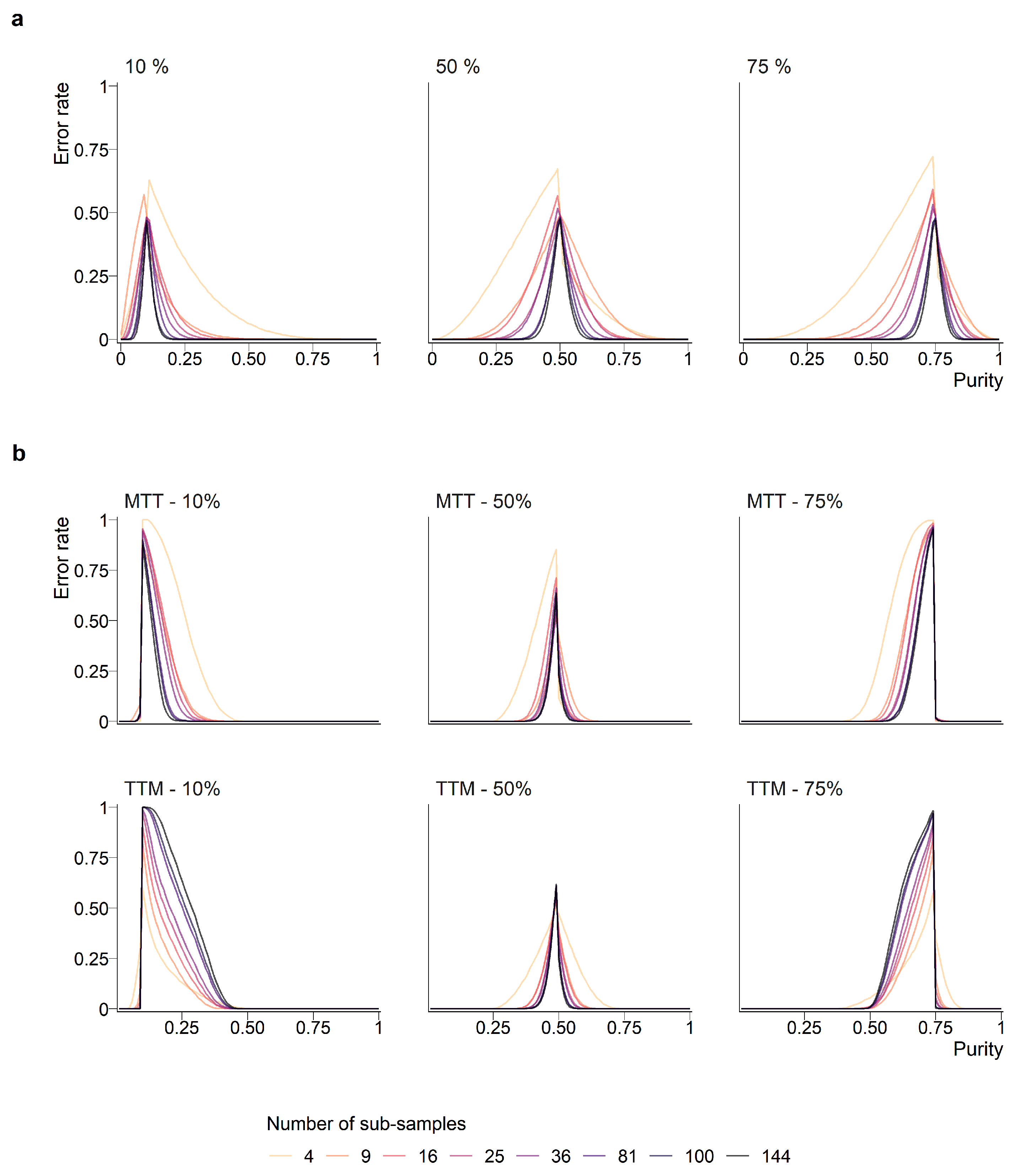
Heterogeneity indices allow us to generalize the overall error rates estimated on the study area. The selected heterogeneity indices, which are independent of the landscape and spatial resolution, highlight the peaks of the labeling uncertainty and the sampling units where the label can be trusted. The error rates are strongly related to the heterogeneity indices of the sampling units for both binary (
, see
Figure 4) and majority classification system (
, see
Figure 5).
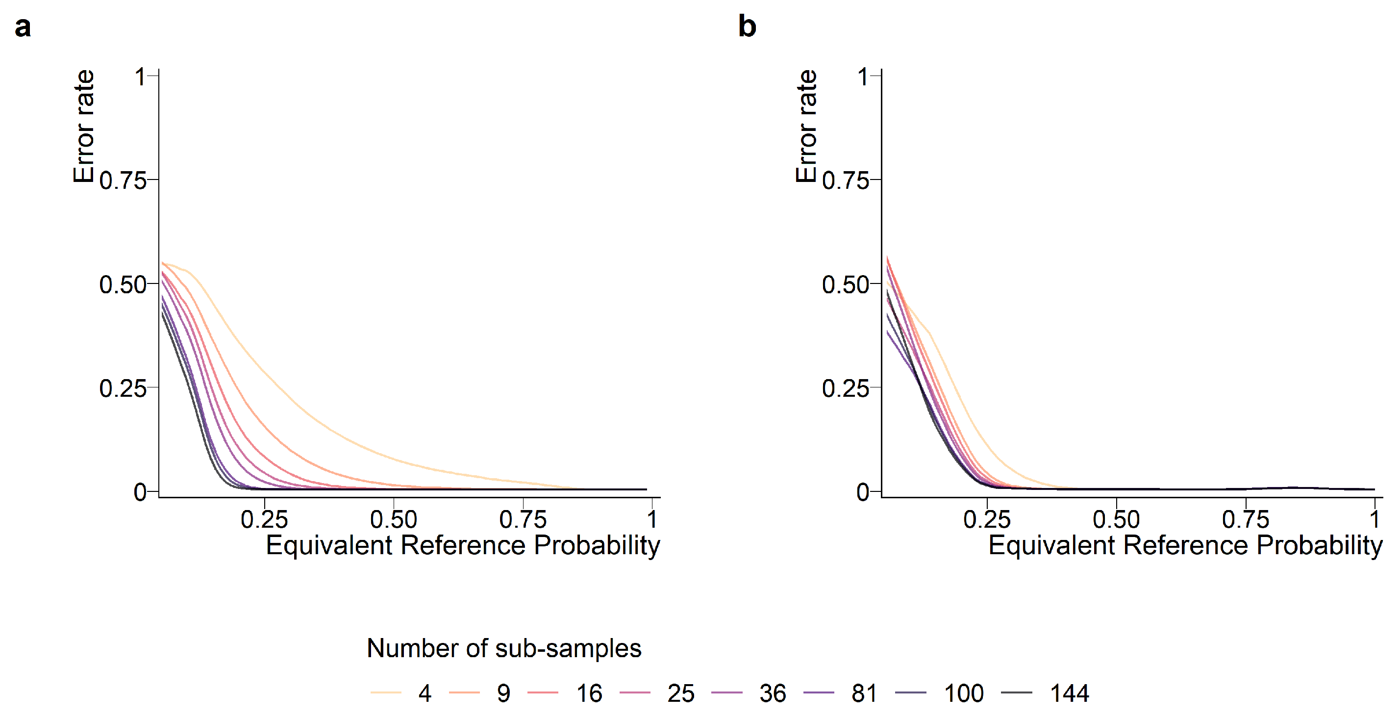
In point-based designs, the error rate is maximum for sampling units with forest proportions close to the class threshold. The error distribution is slightly asymmetric, especially with small sampling efforts, with the longest tail towards the proportion of 50%. Consistently with the expression of the variance for a binomial distribution, the largest variance of the distribution of errors is observed with the 50% threshold and decreased towards the extremities of the range. To achieve an error rate of <1% on average with 16 points, the actual proportion needs to differ from the threshold value by circa 20%.
Thus, the error distribution of partition-based response designs also peaks near threshold values. Our results clearly indicate that the partition-based method are strongly biased when the threshold is not 50%: with thresholds at 10% and 75%, the errors rates increase from 50% towards the value of the threshold, where they are systematically wrong. This is due to the systematic omission of the class that contains the 50% interval when approaching the extremities of the range, which is the only type of error when using a partition-based response design with these threshold values. Indeed, the error rate drops to zero in terms of detection of the class that is located at one end of the interval.
For the majority classification system, the largest error rates are observed for sampling units with similar proportions (low
values). Labeling is 99% correct when the reference equivalent probability is ≥0.5. Interestingly, point-based designs are more accurate than partition-based designs for complex landscapes. On the other hand, designs based on a limited number of partitions outperformed their point-based counterparts for simple landscapes (
). Overall, partition-based designs appear insensitive to an increase above 9 in the number of sub-samples, while larger numbers of sub-samples markedly improve the efficiency of point-based design within the range of values tested in this study. This corroborates the results of overall error rates in the case study (
Table 1).
5.3. Optimization of the Number of Sub-samples
We optimized the number of sub-samples so that the resulting label reached either (1) a 90% or 99.9% confidence level for each sampling unit or (2) the maximum number of sub-samples (144) was attained. The difference between the error rates of the 99.9% optimized and the error rate with a fixed (144) number of sub-samples was <1%.
The regions of high label uncertainty highlighted in
Figure 4 and
Table 1 are consistent with the regions that require more validation efforts (
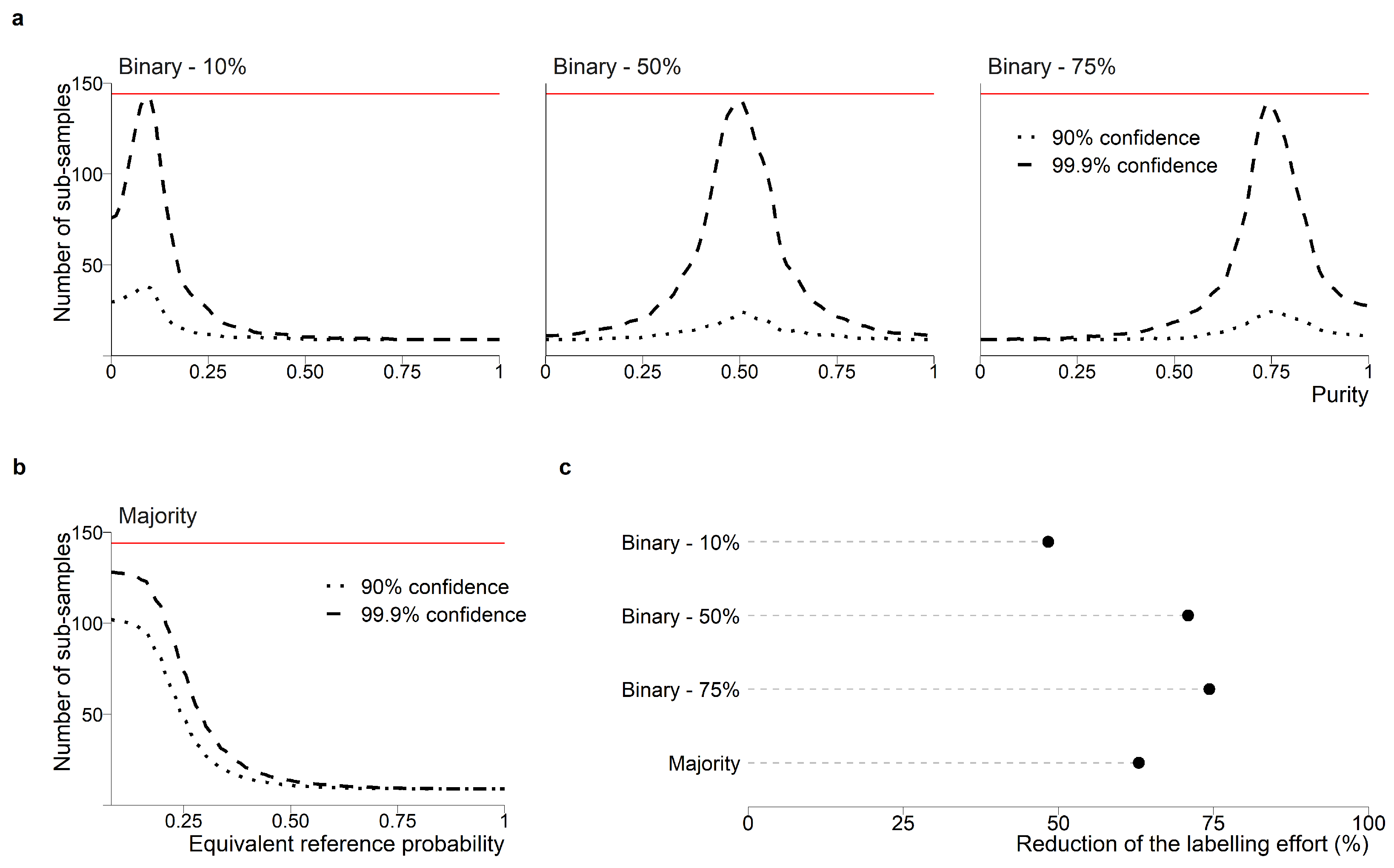
Figure 6a,b). More samples are needed when
is low or
is close to the threshold value. The mean number of sub-samples then decreases quickly, especially with the binary classification systems, so that less than 20 points are needed for most of the range of
or
when the confidence level is set to 99.9%. Furthermore, the 90% confidence level is achieved with low effort for the binary classification systems (
Figure 6a). The sampling effort around the minimum
value for the majority classification system remains high in comparison (
Figure 6b), which is consistent with the larger error rates observed for point-based validation.
The main difference between the shapes of the distribution of the error rates (
Figure 4) compared with the mean optimized number of points (
Figure 6a) occurs on the extreme values of
for the binary classification system. Indeed, the error rate for
value of 0% with 10% threshold (or 100% with threshold 75%) is close to zero, but the number of sub-samples needed to achieve 99.9% confidence is relatively high (75 for the 10% threshold and 40 for the 75% threshold).
In the study area, the optimization method with a very high confidence (99.9%) could more than halve the labeling effort compared to a systematic sub-sampling of 144 sub-samples per sampling unit (
Figure 6c). It required an average of 57, 27 and 26 sub-samples for binary thresholds of 10, 50 and 75%, respectively. The majority classification system was the most difficult to validate, with an average of 115 points needed and the maximum (144) number of sub-samples needed in 56.1% of the sampling units.
The 90% confidence interval could be achieved for the binary classification systems with on average 21, 10 and 11 sub-samples for thresholds of 10, 50 and 75% respectively. For the majority classification system, it required an average of 99 points. Those results are due to the fact that the maximum number of sub-samples (that is 144 in this study) was reached 38% of the cases.
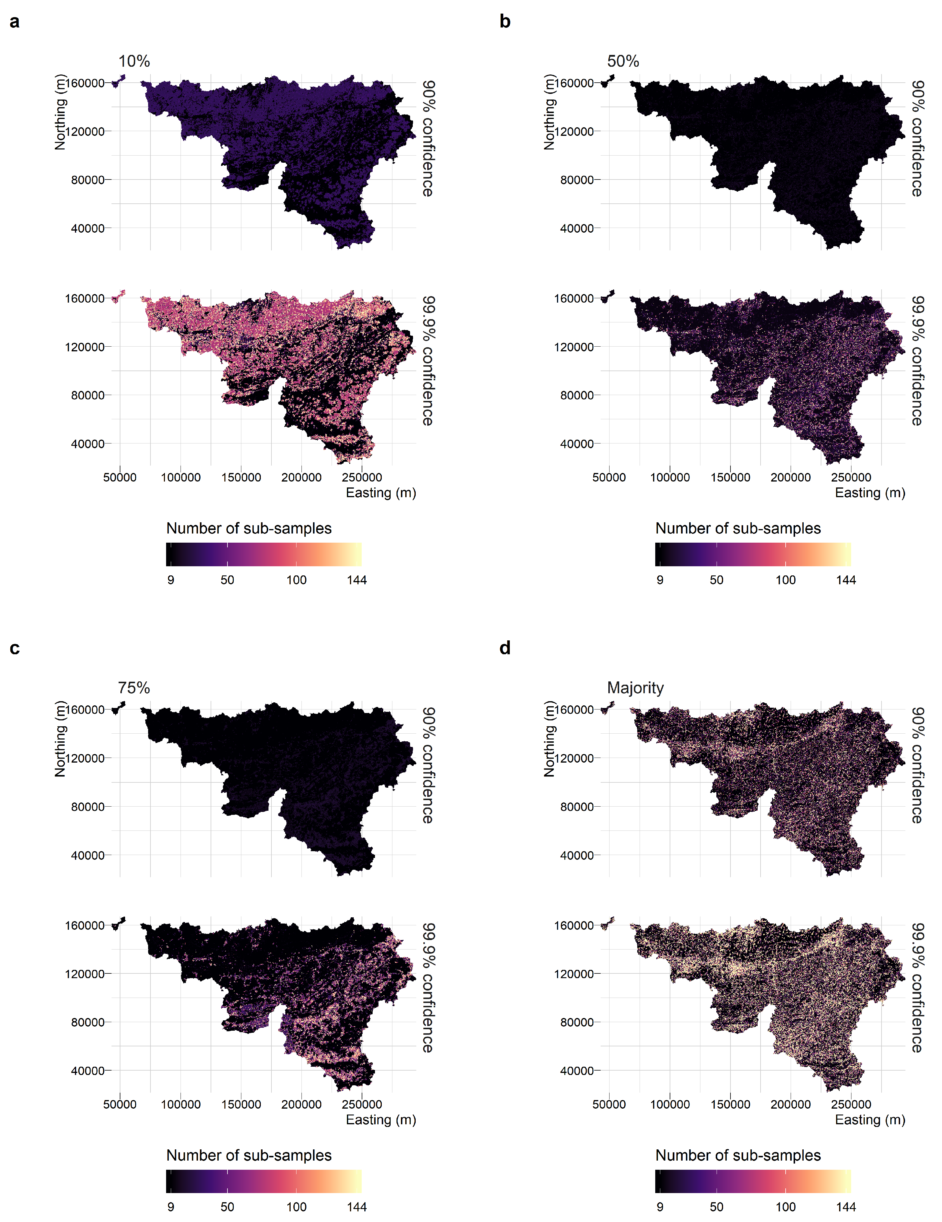
Collecting reference data with a confidence level of 90% can be achieved at a reasonable cost (
Figure 7). The number of sub-samples that is needed to determine the binary class is indeed relatively low (between 9 and 40) over the entire study area, despite the fragmentation of the landscape. For the majority classification system, a spatial pattern of sampling units that need more than 100 sub-samples becomes visible along the main rivers (Meuse and Sambre) and the main cities, where the diversity of land-cover types is the highest.
Reaching a confidence level of 99.9% on the reference data set is much more challenging (
Figure 7). For the majority classification system, the required number of sub-samples is even larger in heterogeneous areas (such as the large urban areas) while only a few patches of homogeneous land-cover types can be validated with as little less than 20 sub-samples. Mapping the required number of sub-samples also highlights the particularities of the landscape in the study area. For instance, the binary classification system is more demanding in open landscapes (for the 10% threshold) or closed forests (for the 75% threshold), when the actual proportions are close to the threshold values. On the other hand, the benefits of the optimization of the number of sub-samples is substantial on large patches where the land-cover proportions are distinct from the threshold value of the classification system. On the study area, the threshold of 75% shows the biggest contrasts between the areas that need a large effort and the areas that can be easily validated. On the other hand, the 50% threshold is most of the time the less demanding in terms of validation effort and mainly requires extra efforts along the forest edges.
6. Discussion
We assessed the accuracy of two main types of quantitative response designs—a set of points and a grid of squares—based on a protocol that provided full control over the validation process. While it is well known that mixed pixels are more difficult to label than pure ones, we quantified how labeling uncertainty increased for class proportions close to the class boundaries. Our results highlight the underestimated difficulty of developing accurate reference data sets for any combination of response design and classification system. Indeed, the required number of sub-samples to reach 98% confidence level was often too high (more than 100 sub-samples per sampling unit) to be practically implemented. When factoring in the cost of response designs with large number of sub-samples, collecting error-free reference data seems barely feasible. Therefore, matching the data collection effort to the available resources appears critical. In other words, there is a necessary sacrifice of the confidence of reference data to achieve rigorous accuracy assessment at reasonable costs.
The efficiency of point-based and partition-based response designs differed depending on the classification system. Partition-based response designs ought to be preferred for majority classification systems and for binary classification systems with threshold values close to 50%. Point-based response designs become more efficient for thresholds that are close to 0% or 100%. The ability to directly determine the class proportions inside a sampling could also help to arbitrate between the two types of partition-based response designs, MTT and TTM, because TTM is much more dependent of the operator skills than the other response designs. Response designs that are solely based on the estimations of the proportions by an operator would however necessitate a specific quality control to evaluate their accuracy.
The main advantage of point-based validation is the possibility to estimate the reliability of the label from the points themselves, and hence to objectively optimize the sub-sampling process without prior knowledge about the sampling units. We demonstrated that relying on a fixed number of sub-samples is inefficient because the same amount of resources is spent to label both homogeneous and complex sampling units. An efficient approach would reduce the effort for those easy-to-interpret cases and allocate it to label complex cases to increase their confidence. To this aim, we propose to iteratively interpret sub-samples until the estimated class proportions reached the desired confidence level. Combined with advanced validation applications, such an approach computes the required number of sub-samples on the fly, thereby reducing the labeling cost as soon as there is no doubt (for a given confidence level) about the label of the sampling units. We showed that, in our study area, the labeling effort could be reduced by 50% to 75% without affecting the accuracy of the labels. As a result, the labeling effort was strongly reduced across the study site and concentrated in the fragmented and ambiguous areas. In some cases, i.e., close to the threshold value, the added value of labeling additional points plateaus because sampling units with proportions close to the classification system definition are always uncertain. Limiting the maximum number of sub-samples to be labelled is thus recommended.
An iterative optimization approach for partition-based designs is impractical because labels could be contradictory when changing scale. Therefore, optimizing partition-based designs would rather depend on subjective operator decision about the proportions she/he estimates inside each sampling unit. Nonetheless, well trained operators could be granted the ability to select several partitions based on their impression of the complexity of the landscape. This method is likely to work well for threshold values near 50% and could avoid extra work in simple cases, but remains sensitive to the Modifiable Area Unit Problem (MAUP) –a statistical biasing effect that occurs when arbitrary units are used to collect data such as class proportions. As described in Jelinski and Wu [
57], the MAUP applies to two types of problems which are relevant in partition-based designs. The first aspect of the MAUP is the “scale problem”, where the same set of areal data is aggregated into several sets of larger areal units, with each combination leading to different data values. The second is the “zoning problem”, where a given set of areal units is recombined into zones that are of the same size but located differently, again resulting in variation in data values. MAUP could be mitigated by generating partitions that correspond to actual image objects derived via segmentation [
46]. Image segmentation has been used in response designs for coarse resolution image validation [
58] and is mainly justified in landscapes that can be divided in a small number of homogeneous patches, not in areas that are very fragmented at a larger scale than the sampling unit. Because of the purity of image-objects derived by image segmentation is usually larger than square cells of the same area [
49], this reduces the uncertainty of the labeling [
59]. However, delineation errors frequently introduce variance and bias on the estimated surfaces of the patches extracted by automated image segmentation [
60]. The accuracy of the response design should therefore be assessed with external data or again rely on an estimation provided by the operator. However, one may lose control over the number of sub-samples generated by the segmentation algorithm, leading to unpractical labeling effort.
In this study, the reported error rates resulted only from imprecise estimation of the class proportions. There are, however, additional errors that should still be considered for a complete understanding of the response design reliability: (1) the simplification of the pixel model, which is a simplified representation of the area observed by remote sensing [
61,
62,
63,
64,
65]; (2) geolocation errors, which further increase the variance of the estimated proportions because the sub-samples may be matched with locations that are outside the sampling unit; and (3) photo-interpretation errors. Indeed, while we assumed that operators made no errors throughout the paper, their performance is in reality imperfect [
23,
46,
66,
67]. For instance, Powell et al. [
23] concluded that five interpreters were required to agree upon a specific class. Human factors are responsible for no less than 20% of the inter-individual differences in operator performance [
10]. To be more realistic, errors rates should account for errors of interpretation of the landscape and, in partition-based designs, errors in estimating the area of each class. As such, the error rates reported in this study are thus lower bounds.
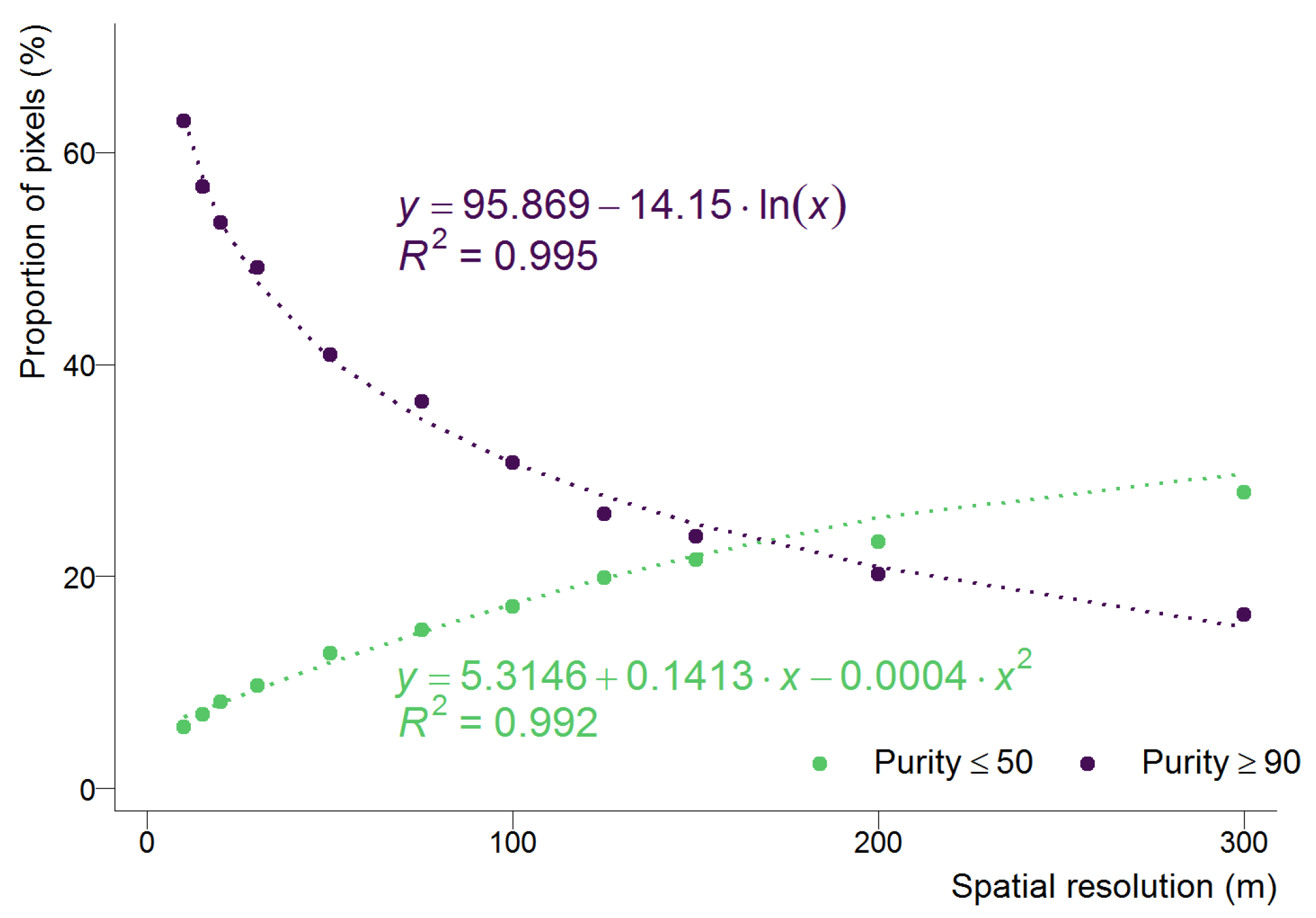
Sampling units of 360 m × 360 m were used because these are divisible by a large number of integers and, therefore, allowed us to easily simulate a large set of regular partition-based designs. While this practical constraint has no direct impact on the generalization of our results, changing the size of sampling units would, however, indirectly impact the response design accuracy. Indeed, the average purity of the sampling units increases when the ratio between the ground sampling distance and the width of the object increases [
62]. This general rule was also observed in our study area, which showed very strong relationship (
) between the pixel purity and the spatial resolution (
Figure 8). If the classification system remains identical, the accuracy of the response design will likely increase for sampling units of higher spatial resolution, and the estimation errors could be neglected when the sampling units become smaller than the spatial objects of interest.
Another solution to minimize the estimation error is to carefully select the classification system with threshold values as far as possible from the modes of the distributions of land-cover proportions. This explained why our results with the binary classification system at 50% threshold was more reliable than the other binary classification systems despite its larger variance on the estimated proportions around the threshold value. In practice, this is not always feasible because it might reduce the fitness for purpose of the map. Besides, the uncertainty of the classification system could become misleading when the study area becomes too large. The preliminary step of defining the classification system is therefore of paramount importance.
In consolidating good practices to collect gold-standard validation data, we demonstrated that the number of sub-samples required to meet stringent confidence levels is often too large to be realistically implemented. Therefore, this work suggests three main directions for future research. First, direct class assessment by operators should be compared with sub-sampling approaches to evaluate the overall level of confidence with real photo-interpretation in both cases. Second, unbiased confusion matrices could be built to account for uncertain reference data. While the errors affecting reference data cannot be predicted, we have however shown that the probability of estimation error could be estimated based on the sub-samples. This information could be used to quantify a large part of the uncertainty of a reference data set at no extra cost. Third, the recent advances in image recognition and computer vision suggest that computer-assisted labeling of sub-samples could help to increase the number of sub-samples at lower cost (see, for instance, [
68]). However, algorithms would need to perform very accurately not to compromise the quality standards of reference data.


