Article

A Mobile LiDAR for Monitoring Mechanically Stabilized Earth Walls with Textured Precast Concrete Panels

1
Lyles School of Civil Engineering, Purdue University, West Lafayette, IN 47907, USA
2
Civil Engineering Department, King Saud University, Riyadh 11421, Saudi Arabia
3
Department of Earth and Environmental Sciences, Yarmouk University, Irbid 21163, Jordan
*
Author to whom correspondence should be addressed.
Remote Sens. 2020, 12(2), 306; https://doi.org/10.3390/rs12020306
Submission received: 6 December 2019 / Revised: 10 January 2020 / Accepted: 15 January 2020 / Published: 17 January 2020
(This article belongs to the Special Issue Remote Sensing for Monitoring Infrastructure Deformation)

Abstract

:
Mechanically Stabilized Earth (MSE) walls retain soil on steep, unstable slopes with crest loads. Over the last decade, they are becoming quite popular due to their high cost-to-benefit ratio, design flexibility, and ease of construction. Like any civil infrastructure, MSE walls need to be continuously monitored according to transportation asset management criteria during and after the construction stage to ensure that their expected serviceability measures are met and to detect design and/or construction issues, which could lead to structural failure. Current approaches for monitoring MSE walls are mostly qualitative (e.g., visual inspection or examination). Besides being time consuming, visual inspection might have inconsistencies due to human subjectivity. This research focuses on a comprehensive strategy using a mobile LiDAR mapping System (MLS) for the acquisition and processing of point clouds covering the MSE wall. The processing strategy delivers a set of global and local performance measure for MSE walls. Moreover, it is also capable of handling MSE walls with smooth or textured panels with the latter being the focus of this research due to its more challenging nature. For this study, an ultra-high-accuracy wheel-based MLS has been developed to efficiently acquire reliable data conducive to the development of the serviceability measures. To illustrate the feasibility of the proposed acquisition/processing strategy, two case studies in this research have been conducted with the first one focusing on the comparative performance of static and mobile LiDAR in terms of the agreement of the derived serviceability measures. The second case study aims at illustrating the feasibility of the proposed strategy in handling large textured MSE walls. Results from both case studies confirm the potential of using MLS for efficient, economic, and reliable monitoring of MSE walls.

1. Introduction

Mechanically Stabilized Earth (MSE) walls have been widely used to stabilize steep, unstable slopes that are subjected to crest loads [1]. Low-cost construction and ease of installation have made MSE walls with precast concrete panels a common infrastructure along transportation corridors within the United States as well as other countries. For instance, in the state of Indiana, USA, there are roughly 1200 to 1500 MSE walls excluding those on Local Public Agency (LPA) routes [2]. An MSE wall is comprised of several components including a façade of precast concrete panels supporting many compacted backfill layers strengthened with geosynthetic or metallic reinforcement [3]. A typical cross-section of the components of an MSE wall is shown in Figure 1. Modular facing blocks, which could be smooth or textured—i.e., with several architectural and aesthetically pleasing finishes, constitute the façade of the MSE wall [4,5]. The key function of these facing panels is preventing backfill soil material from leaking out of the joints. The joints between the panels permit excessive water to seep through them. Failure of an MSE wall can lead to loss of life and/or property damage. Therefore, a monitoring strategy that can quickly, economically, and reliably detect any anomalies in an MSE wall is of high importance.
The long-term performance of an MSE wall relies on a well-designed and constructed system that meets the specifications provided by regulatory organizations such as the U.S. Department of Transportation (DOTs). Internal and external inspections are regularly conducted to ensure the prevention of reinforcement rupture and pullout from the facing panels. A commonly accepted set of serviceability measures include the longitudinal angular distortion ( α L ) and the transversal angular distortion ( α T ) , which have been proposed by the American Association of State Highway and Transportation Officials (AASHTO) [6]. The longitudinal angular distortion ( α L ) is defined as the ratio of the differential settlement between two points along the length of the MSE wall to the horizontal distance between them as illustrated in Figure 2a. The transversal angular distortion ( α T ) is defined as the lateral deflection (i.e., out of the wall plane) of the MSE wall divided by its height, as illustrated in Figure 2b.
Table 1 provides the tolerable α L values for MSE walls that are constructed using incremental precast concrete panels with different joint widths. For the transversal angular distortion, during the construction of an MSE wall with incremental precast concrete panels, the tolerable α T values when measured with a 3.048 m (10 ft) long straight edge should be less than 1/160. At the end of wall construction, α T should be less than 1/240 when measured using a plumb line dropped from the top to the bottom of the constructed wall [6]. In addition to the angular distortions, the U.S. Federal Highway Administration provided guidelines for tolerable out-of-plane offset between neighboring panels [7]. According to such guidelines, the out-of-plane offset at any joint should be less than 9.53 mm (3/8 in) during wall construction. The standard serviceability measures, with the exception of the out-of-plane offset, are global measures focusing on the vertical settlement and lateral deflection of an MSE wall. However, most MSE wall failures are closely related to local deformations, such as relative angular tilt and displacement among neighboring panels, as shown in Figure 3. Therefore, a reliable monitoring should be capable of providing measures that evaluate the deformation behavior of the individual panels within an MSE wall. Examples of such measures are those proposed by Lin et al. [5].
Other than the serviceability measure type, the monitoring strategy should also consider factors that would affect the practical implementation and scalability of such an approach. Total station, geotechnical field instrumentations, and/or static Terrestrial Laser Scanning (TLS) are the most commonly used data acquisition systems for the derivation of the serviceability measures. However, such instruments require access to the MSE wall site and this could subject the inspectors to hazardous conditions as a result of incoming traffic. In addition, field data collection is time consuming; thus, making the monitoring process non-scalable. The third challenge, which should be addressed by a monitoring strategy, is its ability to deal with both smooth and textured MSE walls that could be straight or curved (i.e., the MSE wall is comprised of a set of individual planar faces—Figure 4a—or a single curved façade which could be considered piece-wise planar—Figure 4b). Prior research (e.g., Lin et al. [5]) has mainly dealt with planar MSE walls with smooth panels (i.e., the one in Figure 4a). Therefore, the development of a methodology that could deal with any type of MSE walls would be valuable. In response to existing challenges for monitoring MSE walls, this research is focusing on addressing the following three objectives:
(1)
Development of a monitoring strategy that could be used for the delivery of both standard and recently-available serviceability measures,
(2)
The monitoring strategy is based on reliable, scalable data acquisition procedure—more specifically, point clouds captured by a Mobile LiDAR mapping System (MLS) will be used for serviceability measures derivation, and
(3)
The strategy could handle MSE walls with smooth or textured precast concrete panels along either planar or piece-wise planar façades.
In this paper, Section 2 starts with an overview of existing MSE wall monitoring strategies with an emphasis on those utilizing LiDAR point clouds. Then, the developed MLS data acquisition system and two case studies used in this paper are presented in Section 3. The first one focused on illustrating the fact that an MLS can provide similar performance measures to those derived from TLS. The second case study, on the other hand, aims to illustrate that the data acquisition modality and processing strategy are capable of monitoring large MSE walls along a transportation corridor. The MSE walls considered in both case studies have piece-wise planar façades and are comprised of textured panels. The study then proceeds with the coverage of the proposed methodology in Section 4 and experimental results for the two case studies are discussed in Section 5. Finally, in Section 6, it concludes with the main findings of this study and the recommendations for future research.

2. Related Work

Commonly used MSE wall monitoring techniques are based on visual inspection/examination using a variety of instruments, such as measuring tapes and plumb lines. However, such techniques may have inconsistencies due to human subjectivity that vary over time [8]. Other methods for evaluating some serviceability measures for MSE walls with precast concrete panels include the use of a total station or TLS. Laefer et al. [9] proposed an approach for monitoring retaining walls using TLS. For the data collection, multiple temporal scans are required to detect any movements of the vertically stacked panels within an MSE wall. Each scan must include at least three spherical targets, which are used as reference points for registration/alignment and monitoring purposes. The spherical targets should be placed at the same location for each scanning operation. The study recommended that the targets are left on-site for the duration of the monitoring course. Oskouie et al. [1] utilized TLS to acquire point clouds to derive some performance measures for MSE walls. In their research and before starting any data processing, they first cleaned the data from unwanted objects, such as temporary steel and wooden brackets. Then, a planar model is fitted through the wall using the random sample consensus (RANSAC) algorithm [10]. Based on the distance between the fitted plane surface and the vertical/horizontal joints separating neighboring panels, joint distances are reported. More specifically, vertical/horizontal joints are considered as outliers when inspecting their normal distances relative to the fitted wall plane surface. Lienhart et al. [11] presented a practical approach for large-scale monitoring of retaining walls along Austrian highways using a Mobile Mapping System (MMS). The measurement platform consisted of two laser scan profilers, inertial measurement unit (IMU), differential global navigation satellite system (GNSS) receiver, and multiple cameras. The cameras are utilized to provide true colors for the point clouds. The aligned point clouds from different sensors were used to generate vertical profiles every 5 cm along the retaining wall by intersecting the wall surface model with planes orthogonal to the vehicle’s trajectory. A fitted regression along the vertical profile is then used to derive the tilt angle. They found that it is possible to determine the tilt angle with an accuracy better than 0.1°. However, their approach is limited to evaluating the transversal out-of-plane angle of the retaining wall, which is similar to the AASHTO-based transversal angular distortion ( α T ) . Lin et al. [5] utilized TLS to derive the standard longitudinal and transversal angular distortions of MSE walls with smooth panels. In their work, they also derived new measures that describe out-of-plane angular tilts and displacements of the panels relative to the individual MSE wall faces. For the derivation of the standard and new performance measures, Lin et al. [5] defined coordinate systems for the individual faces and panels, denoted as the Levelled Face ( L F c s ) and Panel ( P c s ) coordinate systems, respectively. L F c s was derived by using a plane fitting through a manually-cropped face of an MSE wall and considering the local horizontal/vertical directions within the site. The definition of the Pcs started with the identification of the individual panels through a region segmentation procedure where the normal distance between the points along the face and the best fitting plane through these points was used as the segmentation criterion. Following the panel segmentation, its bounding box—i.e., Minimum Bounding Rectangle (MBR) [12]—was used to define the P c s . The new serviceability measures developed in their work were based on the spatial and rotational relationships between the L F c s and P c s .
The above literature has already shown the potential of using TLS for MSE wall monitoring while providing high accuracy, reliable serviceability measures. However, the TLS monitoring strategy is time-consuming, limit traffic accessibility, and has not been fully tested when dealing with large MSE walls with either smooth or textured panels. Due to the large number of existing MSE walls, limited monetary resources, and time-critical needs, the frequency of scheduled inspections is not always sufficient to detect problems in a timely manner. In order to verify MSE walls integrity more efficiently, the presented research in this study proposes a monitoring strategy is based on an MLS. Such systems collect high accuracy, high-resolution point clouds in a short time while driving along the transportation corridor. The system description along with the involved case studies are presented next, in Section 3.

3. Data Acquisition System Specifications and Configuration of the Case Studies

The main objective of this research is illustrating the feasibility of using a wheel-based MLS for the acquisition of point clouds that could be used for the derivation of standard as well as recently-available serviceability measures for textured MSE walls. An in-house developed MLS, shown in Figure 5, has been used for the involved case studies. The system is comprised of two high-grade laser scanners (VUX-1HA, Riegl, Horn, Austria and Profiler 9012, ZF, Wangen, Germany) and two rear-looking cameras (two Flea2 5.0MP cameras, FLIR, Wilsonville, OR, USA). Each of the laser scanners has a single laser beam and delivers a 360° horizontal field of view. The Riegl VUX-1HA and ZF Profiler 9012 can capture roughly one million points per second each with a range of 150 m (at an accuracy of ±5 mm) and 120 m (at an accuracy of ±2 mm), respectively [13,14]. The sensors onboard the MLS are directly georeferenced by a ProPak6 GNSS receiver and an ISA-100C near-navigation grade IMU (NovAtel, Calgary, AB, Canada). The accuracy of derived GNSS/INS attitude after post-processing is 0.003° for the pitch/roll angles and 0.004° for the heading (yaw). The positional accuracy, on the other hand, is in the range of 0.01 to 0.02 m [15]. A rigorous system calibration procedure [16] is used for the estimation of the mounting parameters—spatial and rotational offsets—between the GNSS/INS and laser scanning units. The system calibration parameters are estimated through minimizing the discrepancies between conjugate points, linear features, and planar features captured from different drive-runs.
Two textured MSE walls in the state of Indiana were selected to illustrate the feasibility of the developed MLS and proposed processing strategy for deriving both standard (longitudinal and transversal angular distortions) and new performance measures introduced by Lin et al. [5]. Site-1 was selected to evaluate the capability of mobile LiDAR in inspecting an MSE wall by comparing the derived measures to those based on TLS. More specifically, TLS and MLS data were acquired for Site-1. A Focus x330 TLS unit (Faro, Mary, Florida, USA) which has a range accuracy of ±2 mm at 25 m object distance, has been used for the data acquisition at Site-1 [17]. It has a maximum range of 330 m while emitting close to one million pulses per second. This scanner provides color-coded point clouds using a built-in camera. More specifically, at a given location, the TLS performs two consecutive scans with the first one dedicated to acquiring the 3D point cloud, while the second scan captures successive images that are used for colorizing the individual points. For Site-2, the dataset, which is only captured by the MLS, is used to evaluate the performance of mobile LiDAR when dealing with large MSE walls. Figure 6a,b) show a photo of a portion of the textured MSE walls at Site-1 and Site-2, respectively. As it can be seen in Figure 6, both MSE walls have textured panels and are piece-wise planar façades (i.e., the façades cannot be modeled as a single planar surface).
The textured MSE wall at Site-1 was built in 2017 and is comprised of a single side with piece-wise planar façade. The total length along the MSE wall is approximately 175 m with a height of 4.5 m. The MSE wall facing consists of 85 rectangular precast textured concrete panels that are approximately 1.5 m by 3 m in size. The width of the panel joints for the size of the facing panel used in this wall is 19 mm (0.75 in.) as prescribed in the Indiana Department of Transportation standard specifications [18]. Two TLS scans were conducted in order to obtain full coverage of the MSE wall and mitigate any occlusions caused by vegetation and/or road furniture (e.g., light poles and signs). The MLS system drove forward and backward, as shown in Figure 7a. The MLS dataset contains point clouds captured in the two drive runs at an average driving speed of 15 mph collected over almost 30 s. A sample of the collected point cloud is shown in Figure 8a.
Figure 6b shows a photo of the MSE wall at Site-2. The wall was built in 2014 and has two sides (denoted hereafter as Side A and Side B) (see Figure 8b), with a length of 175 m and an average height of 7.5 m. The MSE wall has a total of 296 panels on Side A and 80 panels on Side B. Figure 7b shows the path of the vehicle travelled during the data collection. The dataset has four drive runs captured at an average driving speed of 25 mph for over almost 30 s. The double drive runs in each driving direction as well as the forward and backward drive runs provide a data redundancy, which could mitigate potential occlusions from nearby objects and degraded resolution from varying scanner-to-object distance. An example of the MLS point cloud for two drive runs at Site-2 is shown in Figure 8b.

4. Methodology

4.1. Conceptual Basis of the Proposed Methodology

In this research, a scalable, systematic approach for MLS-based monitoring of large MSE walls with textured precast concrete panels is developed. A flowchart of the proposed procedure, comprising data acquisition, data processing, and estimation of performance/serviceability measures for MSE walls, is shown in Figure 9. As previously mentioned, the standard serviceability measures, as proposed by AASHTO [6], evaluate the longitudinal and transversal angular distortions of a given MSE wall face. The newly developed serviceability measures by Lin et al. [5] provide the relative displacement and rotation of the individual panels relative to a Levelled Face coordinate system ( L F c s ) . The developed strategy is designed to be capable of handling MSE walls that have either smooth or textured precast concrete panels. Moreover, it can handle MSE walls with fully planar or piece-wise planar façades. Finally, the input point clouds to the processing methodology could be either from MLS or TLS data acquisition systems.
In order to derive the performance measures, the point clouds captured from different MLS drive runs or TLS scans need to be registered to a common reference frame. When using a TLS unit, acquiring several laser scans with significant overlap is a fundamental requirement for guaranteeing full coverage of the site of interest. The outcome from a TLS scan is a 3D point cloud referenced to a local coordinate system associated with the scanner’s location and orientation. Hence, a registration process must be performed when dealing with multiple TLS scans in order to align them relative to a common reference frame.
Theoretically, registration is not necessary for point clouds acquired by an MLS since they are directly georeferenced through the onboard GNSS/INS unit. More specifically, the GNSS/INS trajectory, when combined with the system calibration parameters, produces the position and orientation of the laser scanners relative to the mapping frame (e.g., the UTM coordinate system with the WGS84 as the datum for horizontal coordinates and the National American Vertical Datum of 1988—NAVD 88—for vertical coordinate). Therefore, collected point clouds from different drive runs should be properly aligned as long as there is reliable trajectory data and access to accurate system calibration parameters. However, issues related to canopy cover, obstructions (e.g., tunnels and/or overhead bridges), GNSS-signal multipath interference from neighboring traffic, and platform speed could compromise the GNSS/INS trajectory would lead to alignment discrepancies between overlapping point clouds from neighboring drive runs. To take advantage of the available/complementary point cloud data from multiple drive runs, fine alignment must be ensured (i.e., a fine registration must be conducted to ensure the alignment of the point clouds from the different drive runs).
Regardless whether point clouds were acquired by TLS or MLS units, alignment must be ensured through a registration procedure. In general, registration strategies can be categorized into coarse and fine approaches [19,20]. Since this research primarily utilizes MLS point cloud data, which is aligned to a high degree by the onboard GNSS/INS unit, we focus on fine registration. The point cloud fine registration strategy adopted in this research is discussed in more detail in Section 4.2.
Once the point clouds of the MSE wall in question have been accurately registered, we proceed with the identification of individual planar segments of the wall. In other words, if an MSE wall is multi-face with planar individual faces as shown in Figure 4a or piece-wise planar façade as shown in Figure 4b, it should be partitioned into sections that are believed to be perfectly planar. Each planar section will be denoted hereafter as an MSE wall face. In this research, the identification/partitioning of MSE wall faces is conducted manually. The criterion for the fine-tuning of the partitioning process is based on the Root Mean Square Error (RMSE) of the normal distances between the constituent points from the corresponding best-fitting plane through the MSE wall face in question.
The next step is to define the coordinate systems associated with the MSE wall face (the Levelled Face coordinate system ( L F c s ) ) as well as the individual panels (the Panel coordinate system). These coordinate systems are essential for determining the standard and new serviceability measures. The L F c s is defined by the local horizontal/vertical directions at the MSE wall site as well as the best fitting plane through the face in question, as depicted in Figure 10. More specifically, the Y-axis of the LFcs is defined in a way that it belongs to the MSE wall face (as defined by the fitted plane parameters) and is parallel to the horizontal plane as described by the XY-plane of the defined mapping coordinate system at the site location. The Z-axis of the LFcs is aligned along the vertical direction, i.e., the plumb line, at the MSE wall site. Finally, the X-axis of the LFcs is derived to define a right-handed coordinate system. To facilitate the definition of the LFcs, the geo-referencing parameters from the MLS have to be defined in a local mapping coordinate system with its Z-axis pointing in the local level (plumb line) direction at the MSE wall site location. The panel coordinate system (Pcs) defines the position and the orientation of individual panels, and it is essential for evaluating the relative displacement between the panels as well as the relative displacement/rotation between the panels and the Levelled Face coordinate system, LFcs. As shown in Figure 10, the panel coordinate system is defined in such a way that two of its axes are aligned along the bottom and left sides of the bounding rectangle enclosing the panel. The X-axis of the panel coordinate system is derived to define a right-handed coordinate system (i.e., it is defined by the normal to the panel surface). A key component for reliable derivation of the serviceability measures is ensuring that the Panel coordinate system (Pcs) is defined in an identical manner for all the panels in a given face. To isolate the points making up the individual panels and define the Panel coordinate systems, Lin et al. [5] adopted a region-growing segmentation procedure which utilizes the local point spacing and normal distance from the best-fitting plane to the MSE wall face as the similarity criteria. The underlying assumption for such segmentation is that excessive normal distances from the best-fitting plane correspond to the joints separating the individual panels. Nevertheless, such planar segmentation would not accurately isolate the individual panels for a textured wall as the joints among the panels might not be as distinguishable from the wall texture. In this research, a unique panel identification strategy has been developed to cope with the imposed challenge by working with a textured MSE wall. In this strategy, a region-growing segmentation is first applied to obtain an approximation of the individual panels. A template matching procedure is then performed to refine the panel extraction result, assuming that the individual panels are identical (i.e., the same form is used for panel casting). Section 4.3 describes the proposed face and panel extraction strategy in detail. Finally, after the coordinate systems are established and the individual panels are extracted, the performance measures can be derived. The derivation of the standard and new performance measures for textured MSE walls are presented in Section 4.4.

4.2. Registration of Point Clouds from Different MLS Drive Runs and TLS Scans

As mentioned earlier, the first step towards deriving the performance measures for an MSE wall is to ensure an accurate registration of LiDAR point clouds captured from different MLS drive runs or different TLS scans. A wide range of point cloud registration procedures have been proposed in the past few years. According to Habib and Al-Ruzouq [21], a comprehensive registration paradigm should address four criteria: (1) transformation parameters relating the reference frames of the involved datasets, (2) registration primitives used for the estimation of the transformation parameters, (3) mathematical constraints describing the similarity metric between conjugate primitives after registration, and (4) matching strategy controlling the framework for the automated identification of conjugate primitives. Due to the short duration for the acquisition of the point cloud from different MLS drive runs (e.g., less than thirty seconds for the involved case studies), a 6-parameter transformation (i.e., three shifts and three rotation angles—denoted hereafter as XT, YT, ZT, Ω, Φ, and Κ) would be sufficient. For fine registration, point primitives are recommended since the huge redundancy furnished by the size of the point cloud would ensure the highest accuracy possible for the estimated transformation parameters even though a point-to-point correspondence cannot be guaranteed in the data from different drive runs. Moreover, the similarity metric could be modified to handle point primitives without assuming point-to-point correspondence. The similarity metric could be based on constraining the distance between a point in one drive run and its corresponding point, which is established by the matching strategy, after the application of the transformation parameters to be zero. Addressing the matching strategy is the last task to carry out the alignment process. The well-known iterative closest point (ICP) method [22] can establish the matches through iterative minimization of the squared sum of the point-to-point distances in the overlap area between the different drive runs. A better matching strategy that avoids the underlying assumption of having point-to-point correspondences is the iterative closest patch (ICPatch) [23], which is a variant of the ICP. Within the ICPatch, points in one drive run are matched to triangular patches in another drive run. These triangular patches could be derived through a triangular irregular network (TIN) procedure. In this case, the matching strategy identifies point-patch pairs through the iterative minimization of the squared sum of the normal distances between such pairs. To avoid the TIN generation procedure, which could only handle surfaces with predominantly mild slopes, the iterative closest projected point (ICPP) was developed [19]. In this case, the patch is defined by the closest three points in the second drive run to a transformed point from the first one using the current estimate of the transformation parameters. The matching strategy aims at identifying the matches and estimating the transformation parameters through the iterative minimization of the squared sum of the normal distances between the points in one drive run and their corresponding patch defined by the closest three points in the other drive run [19].
In this research, a modified matching strategy, which is a hybrid implementation of the ICPatch and ICPP, is used. More specifically, the procedure starts with an approximate estimate of the transformation parameters between the captured point clouds from different drive runs. Given that these point clouds are aligned to a high degree through the onboard GNSS/INS, zero shifts and zero rotation angles could be used as the initial values for the transformation parameters. Such parameters are used to transform a point from one drive run—denoted as the source surface—to the reference frame of the other drive run—denoted as the reference surface. The transformed point (Pt) will be used to identify the three closest points in the reference surface. The closest three points will be accepted as a possible match if (Pt) belongs to a bipyramid formed by these points and two vertices that belong to the orthogonal to the triangle defined by these three points through its centroid given a predefined normal distance threshold (Figure 11). The normal distance threshold (n) is selected based on the noise level within the data. Rather than minimizing the squared sum of the distances between the transformed point and its projection onto the corresponding triangle (which is implemented in the ICPP), this research utilized the modified weigh function proposed by the ICPatch for the estimation process. For more details regarding the modified weight function, interested readers can refer to [23].
Compared to the original ICPatch and ICPP procedures, the advantages of the hybrid approach include a higher computational efficiency, less sensitivity to the existence of erroneous points (i.e., outliers), and capability of registering vertical surfaces, which cannot be effectively handled in the original ICPatch. An example of the outcome from the point cloud registration is shown in Figure 12, where two TLS scans at Site-1 are registered together with the MLS point clouds from different drive runs.

4.3. MSE Wall Face and Panel Extraction

In this section, a semi-automated procedure is introduced to extract the faces and the panels of the MSE wall. First, the MSE wall needs to be divided into individual faces that can be considered as planar segments (Figure 13), which corresponds to the MSE wall façade in Figure 4b. The sectioning process is conducted manually and the planarity of each individual MSE wall face is examined by applying a plane fitting to the constituent points. A sectioning/partitioning would be accepted if the root mean square error (RMSE) of the normal distance of the points from the best-fitting plane through this section is below a threshold that depends on the noise level in the data and the texturing detail in the panels. Once the individual faces are established, one can proceed with defining the Levelled Face coordinate system (LFcs) as explained in Section 4.1. Then, a region-growing segmentation technique is applied to segment the points comprising the individual panels as described by Habib and Lin [24]. The similarity criteria for the region growing process include the local point spacing and normal distance between the points and the fitted plane through the face. For a smooth MSE wall face, such criteria can effectively segment the individual panels, and the Panel coordinate system (Pcs) is simply defined by identifying the Minimum Bounding Rectangle (MBR) enclosing the segmented panels, as proposed by Lin et al. [5]. Defining the panel coordinate system in a unique manner for textured MSE walls is much more challenging. The planar segmentation technique mentioned above would not isolate the individual panels in a unique way as the joints among the panels could not be easily identified as out of plane features since their normal distances could be within the texture level of the wall (for example see Figure 14). Moreover, existing occlusions could also affect the segmentation of the complete panels as shown in Figure 15. Therefore, a strategy based on template matching to refine the initial panel segmentation result and uniquely define the Panel coordinate system (Pcs) is proposed.
The initially segmented panels are used to extract the approximate corners, which represent the enclosing rectangle, of the individual panels through a search procedure starting from virtual points that are defined by the minimum/maximum coordinates of the segmented points. These corners are then utilized to define an approximate Pcs for the individual panels and to isolate the point clouds pertaining to the individual panels. Due to the subjectivity of the segmentation procedure and consequently the defined panel corners, one cannot assume that the Pcs is defined in a unique manner for the different panels. To resolve this issue, a panel matching procedure is carried out while assuming that the individual panels are identical (i.e., the same form is used for panel casting). More specifically, a master panel is selected and used as a template for a panel matching procedure. The master panel is denoted as the “template panel” with its Pcs denoted as ( x p t ,   y p t ,   z p t ). The remaining panels are denoted as “matching panels” with their approximate Pcs denoted as ( x p m _ a ,   y p m _ a ,   z p m _ a ). The template and matching Pcs are defined using the corners of the respective panels (i.e., the origin is defined at the lower left corner of the segmented panel; the Y and Z axes are defined by the lines connecting the lower corners and left corners, respectively; and the X-axis defines a right-handed coordinate system). To identify the panels’ corners in a unique manner, the points enclosed by the template and matching panels undergo a registration procedure using the modified ICPatch to estimate the shifts and rotations—as seen in Equation (1)—relating the template Pcs and approximate matching Pcs. In this equation, i is the index of a point that have been matched in the template and matching panels—denoted by k.
r i p m _ a _ k = r p t p m _ a _ k + R p t p m _ a _ k r i p t
where: r i p m _ a _ k : are the coordinates of point i relative to the approximate matching Pcs for the kth panel; r p t p m _ a _ k : are the shifts between the template Pcs and the approximate matching Pcs for the kth panel; R p t p m _ a _ k : is the rotation matrix between the template Pcs and approximate matching Pcs for the kth panel and r i p t : are the coordinates of point i relative to the template Pcs.
Following the estimation of the shifts and rotations relating the template Pcs and approximate matching Pcs, the parameters can be utilized to derive the corners for the matching panels—which correspond to those used for defining the template panel as shown in Figure 16. Using these corners, the Pcs is defined in a unique manner for all the panels along the MSE wall.

4.4. MSE Derivation of Standard and New Serviceability Measures

The standard serviceability measures include the longitudinal angular distortions ( α L ) and the transversal angular distortions ( α T ) . The derivation of such measures is based on establishing longitudinal and transversal lines along the MSE wall face in question. The longitudinal lines are established using the corners of the horizontal edges of all the panels adjacent to these lines by applying a line fitting technique. Once the line parameters (i.e., directional vector of the 3D line) are estimated, a dot product between the directional line parameters and Y-axis components of the LFcs is used to obtain the longitudinal angular distortion ( α L ) . The transversal lines for the columns of panels are derived using the midpoints of the horizontal edges of the uppermost and the lowermost panels of a given column. Then, a dot product of a vector connecting the midpoints of the uppermost and the lowermost panel edges and the Z-axis components of the LFcs is performed to obtain the transversal angular distortion ( α T ) . An example of the longitudinal and transversal lines used for a planar face of the MSE wall at Site-1 is illustrated in Figure 17.
The recently developed serviceability measures by Lin et al. [5] evaluate the relative displacement and rotations of a panel relative to the Levelled Face coordinate system (LFcs). To derive these serviceability measures, the spatial and rotational relationships between the LFcs and Pcs as seen in Figure 18 are utilized. More specifically, the location of the origin of the Pcs relative to the LFcs—denoted as Xo, Yo, and Zo—defines the panel position. The rotation angles—denoted as θ x p , θ y P , and θ z P —that need to be applied to the L F c s to make it parallel to the P c s are used to define the panel orientation. The final measure is the normal distances between the corners of each panel and the fitted planes through the corners of neighboring panels. Using the derived corners from the template matching procedure, one can derive these normal distances as shown in Figure 19. In this figure, eight normal distances—denoted by the red lines—from the four corners of panel 4 to neighboring panels can be estimated (i.e., panels 1, 2, 3, 5, 6, and 7). One should note that using the corners enclosing the panels to define the panel position, orientation, and displacement would exclude the panel texture from impacting the derived measures.

5. Experimental Results

Two case studies were carried out to evaluate the capability of the MLS in monitoring MSE walls with textured precast concrete panels. The case study at Site-1 validates the MLS derived measures by comparing them against those derived from an -TLS dataset. The case study at Site-2 further highlights the capability of the MLS by applying the proposed strategy for inspecting a large textured MSE wall.

5.1. Experimental Results for Site-1

5.1.1. LiDAR Point Cloud Alignment

Point cloud registration was performed to register (i) MLS point clouds from the two scanners onboard the data acquisition system in a given drive run, (ii) the MLS point clouds from two drive runs, (iii) the TLS point clouds from two scans, and (iv) the MLS and TLS point clouds. The estimated transformation parameters relating the derived point clouds from the two MLS scanners in a given drive run can be used to evaluate the quality of the system calibration procedure (i.e., significant deviations from zero shifts and zero rotation is an indication of residual artifacts in the system calibration parameters). The estimated transformation parameters between the point clouds from different drive runs were used to quantitatively evaluate the quality of the GNSS/INS trajectory (i.e., significant deviations from zero shifts and zero rotation is an indication of inferior quality of the GNSS/INS trajectory). The registration of the TLS and MLS point clouds is done to ensure that there are uniquely defined local vertical and local horizontal directions within the study site.
To evaluate the comparative performance of TLS-based and MLS-based inspection strategies, the experimental results for this dataset focused on a single face of the wall that has 32 panels. As already mentioned, this research had two MLS drive runs in opposite directions covering the MSE wall. For the MLS registration process, a total of three registration steps are conducted. The first and second steps involved the registration of the Riegl and ZF scans in each drive run. The third step performed the alignment between the combined/registered scans from the two drive runs. For the TLS, the two scans were registered. Finally, the TLS and MLS point clouds were registered to a common reference frame defined by the latter. Figure 20, Figure 21, Figure 22 and Figure 23 qualitatively illustrate the alignment of the derived point clouds from the two scanners in a given run, point clouds from two different runs in opposite directions, point clouds from the two TLS scans, and point clouds from TLS and MLS units. In each of these figures, four vertical profiles were manually extracted to illustrate the alignment quality. These profiles exhibit an overall alignment, which is commensurate with the expected accuracy range of the individual system, between point clouds from the scanners in a given drive run, two drive runs, two TLS scans, and the TLS/MLS units.
Table 2, Table 3, Table 4 and Table 5 show the respective transformation parameters along with the square root of a-posteriori variance factor ( σ ° ^ ) and average/root mean square error (RMSE) of the normal distances between the registered point clouds in Figure 20, Figure 21, Figure 22 and Figure 23. Close inspection of Figure 20, Figure 21, Figure 22 and Figure 23, and Table 2, Table 3, Table 4 and Table 5 reveals the following:
  • The estimated magnitude of the transformation parameters necessary for the alignment of the Riegl and ZF scanner point clouds indicates the high quality of the system calibration as indicated by small values of these parameters (the estimated parameters are in the range of 2 cm and 0.02°).
  • The estimated transformation parameters necessary for the alignment of the MLS point clouds from different drive runs indicate the presence of some discrepancies between these point clouds in the range of 3 to 5 cm and −0.01° to 0.19°. These are mainly caused by the impact of environmental factors on the GNSS/INS trajectory derivation.
  • The reported square root of a-posteriori variance factor ( σ ° ^ ) and average/root mean square error (RMSE) of the normal distances between conjugate primitives for the different point clouds show the alignment quality following the registration process (i.e., in the 1 to 2 cm range).

5.1.2. Serviceability Measures

Figure 24 illustrates the longitudinal and transversal angular distortions for the textured MSE wall planar face (TLS in green and MLS in blue) as well as the recommended tolerable angular distortions (denoted by the red lines). These angular distortions are evaluated using the longitudinal and transversal lines in Figure 17. The horizontal line in Figure 24a represents the tolerable longitudinal distortions for a joint width of 19 mm (0.75 in.), while the horizontal lines in Figure 24b represent the tolerable transversal angular distortions, as prescribed in AASHTO (2014). Figure 24 reveals that the angular distortions (both longitudinal and transversal) obtained from the MLS closely resemble those derived using the TLS. This confirms the capability of mobile LiDAR in achieving high quality assessment of the standard serviceability measures. As far as the MSE wall evaluation is concerned, Figure 24a,b show that this wall satisfied the longitudinal angular distortion criterion for a joint width of 19 mm (0.75 in.). However, it failed to meet the tolerable transversal angular distortion criterion of 1/240.
As for the recently available serviceability measures, the estimated values (namely, the position of the most lower left corner of each panel—Xo, Yo, and Zo—and the angular orientation of each panel— θ x P , θ y P , and θ z P —relating the P c s and L F c s coordinate systems) are listed in Table 6 for TLS and MLS, respectively. For a perfectly constructed MSE wall, the X-coordinate of the origin of the Pcs relative to the L F c s , denoted as Xo, should be close to zero. Moreover, the YZ-coordinates of the origin of the P c s , denoted as Yo and Zo, should reflect the dimensions of the panels as well as the gap between the panels along the width and height directions, respectively. The position of the panel can be used to detect potential relative movements among the panels in a given face. Such movement can be identified and quantified through repetitive scans over time. The second set of measures is the angular rotations representing the relationship between the L F c s and P c s . As mentioned earlier, the rotation angles θ x P , θ y P , and θ z P represent the rotations that need to be applied to the L F c s until it is parallel to the P c s . More specifically, θ y P and θ z P can be viewed as rotations of the panel out of the L F c s , while θ x P represents a rotation in the plane of the panel. For a perfectly constructed MSE wall, these rotation angles should be as close to zero as possible. Although it is instructive to inspect the data provided in Table 6 for the 32 panels constituting the textured MSE wall face in question, a graphical summary is much more intuitive for identifying trends and outliers. Figure 25 shows the Cumulative Distribution Functions (CDF) for the three angular values ( θ x P , θ y P , and θ z P ) and the panel-to-panel normal distance of TLS and MLS datasets.
Table 7 provides summary statistics of the proposed serviceability measures for the investigated 32 MSE wall panels using TLS and MLS point clouds, respectively. For TLS-based derivation measures, the 95th percentile values of angular tilts ( θ x P , θ y P , and θ z P ) are 0.62°, 0.15°, and 0.63°, respectively. These values almost agree with same measures derived from MLS-based. For the TLS/MLS comparative evaluation, Table 8 shows the statistics of the differences between the TLS-based and the MLS-based serviceability measures. In this table, it can be concluded that MLS-based similarity measures are within 5 cm and 0.5° when compared to those from TLS.

5.2. Experimental Results for Site-2

This dataset is used to further highlight the MLS capability in deriving serviceability measures for a large textured MSE wall. As previously mentioned, the MSE wall at Site-2 has a total of 376 panels along two sides (296 panels along Side A and 80 panels along Side B). There are a total of 4 drive runs in two opposite directions—two drive runs in each direction—covering the MSE wall. The drive runs in each direction cover only one side of the MSE wall. Side A and Side B are sectioned into 6 and 4 planar faces, respectively. To illustrate some of the results from the proposed processing strategy, the following discussion focuses on one face with 31 panels. For the overall summary statistics, the serviceability measures for 285 of the 376 panels are reported (incomplete and partially occluded panels were excluded).
Similar to the processing workflow for Site-1, the registration between the two scanners (i.e., Riegl and ZF sensors) in a given drive run was first performed. Then, the point clouds from the different drive runs were registered. In total, there were three registration steps for the MLS scans in a given direction (two steps for the registration of the Riegl and ZF scans in each of the two drive runs in that direction and the third step for the alignment of the combined/registered scans from those drive runs). Qualitative evaluation of the alignment following the registration procedure when applied to the scanners’ point clouds in a given run and the point clouds from two drive runs is shown in Figure 26 and Figure 27, respectively. The two different colors (e.g., red and blue) in Figure 26 and Figure 27 represent two scanners and two different drive runs, respectively. In those figures, four cross-sectional profiles are used to illustrate the alignment quality. The estimated transformation parameters together with the associated statistics are shown in Table 9 and Table 10. Inspection of the profile alignment in Figure 26 and Figure 27 as well as the reported transformation parameters in Table 9 and Table 10 further confirms the derived observations from Site-1; namely, high quality of the system calibration parameters, small discrepancies caused by the GNSS/INS trajectory, and very good alignment following the registration process.
Following the registration of the different point clouds, this research proceeds by deriving the different serviceability measures. The established longitudinal and transversal lines in Figure 28 are used for evaluating the angular distortions for one of the MSE wall faces at Site-2. Figure 29 illustrates the longitudinal and transversal angular distortions for that face as well as the tolerable angular distortions (i.e., denoted by red lines). The horizontal line in Figure 29a represents the tolerable longitudinal distortions for a joint width of 19 mm (0.75 in.), while the horizontal lines in Figure 29b represent the tolerable transversal angular distortions, as prescribed in AASHTO [6]. As shown in Figure 29a,b, this MSE wall face satisfied the longitudinal angular distortion criterion for a joint width of 19 mm (0.75 in.). However, it failed to meet the tolerable transversal angular distortion criterion of 1/240.
The estimated values of the other serviceability measures (namely, the position of the most lower left corner of each panel—Xo, Yo, and, Zo—and the angular orientation of each panel— θ x P , θ y P , and θ z P —relating the LFcs and Pcs coordinate systems) for the illustrative face with 31 panels are listed in Table 11.
Table 12 provides statistics of the proposed serviceability measures for all the complete/non-occluded panels of the textured MSE wall at Site-2 (285 panels). Although it is instructive to inspect the data provided in Table 12 for all the panels constituting the textured MSE wall, a graphical summary is much more intuitive for identifying trends and outliers. Figure 30 shows the Cumulative Distribution Functions (CDF) for the three angular values ( θ x P , θ y P , and θ z P ) and the panel-to-panel normal distance of the MLS dataset at this site. One of the basic assumptions of MSE walls is that the joints (i.e., gaps) between panels are sufficiently close and have minimal offset along the X-axis of the Pcs between neighboring panels—according to FHWA (2009). It can be concluded from this table that 75% of the panels have an offset less than 0.6 cm, which indicates that the wall meets tolerable out-plane offset as prescribed by FHWA (2009).

6. Conclusions and Recommendations for Future Work

MSE walls are a commonly-used civil infrastructure due to their economic benefits, ease of construction, and accommodating tight right-of-way constraints. Continuous monitoring of MSE walls is necessary to ensure their performance using a wide range of serviceability measures that describe both global and local deformations within the wall. Current approaches for MSE wall monitoring are time consuming, limit access to transportation corridors, and could subject the inspectors and/or instrument operators to risk from incoming traffic. Prior research has shown that TLS is a promising tool for deriving standard/global and new/local serviceability measures. The time-consuming nature of scanner set-up and data collection makes it an impractical approach that could not be scalable. Therefore, this research has proposed the use of MLS for the data acquisition and introduced a processing framework that could produce all types of serviceability measures. Achieving the research objectives has been tested through two case studies with the first one evaluating the comparative performance of TLS and MLS data acquisition modalities. The second case study aimed at illustrating the feasibility of using MLS for monitoring large MSE walls. The key findings/contributions of the proposed acquisition/processing strategy can be summarized as follows:
(1)
Illustrating the potential of Mobile LiDAR in collecting point clouds with sufficient point density to derive global and local serviceability measures;
(2)
Introducing a framework for point cloud processing, which include registration, segmentation, panel isolation, and serviceability measures evaluation, more specifically:
(a)
A hybrid approach has been introduced for the fine registration of scans from different sensors in a given drive run and scans from different drive runs;
(b)
A rigorous procedure has been devised to identify/isolate the individual panels along the MSE wall in a unique manner. For this task, a template matching procedure has been developed to ensure consistent definition of the individual panels along the wall;
(c)
The extracted panels are then used to derive both global and local serviceability measures;
(3)
With an accurate system calibration and high quality GNSS/INS onboard the Mobile LiDAR System (MLS), point clouds from different sensors and different drive runs are shown to enhance the level of the detail in the collected point clouds;
(4)
The potential of MLS has been evaluated through comparative evaluation with TLS—derived serviceability measures from TLS and MLS are in close agreement;
(5)
Extensive testing with multiple real datasets has shown the feasibility of the different components of the proposed processing strategy. To the best of the authors’ knowledge, this is the first study of its kind (i.e., first study that has verified the ability of mobile LiDAR in the acquisition and generation of wide-range of serviceability measures for textured MSE walls).
The proposed methodology in this research can be used to establish acceptance criteria for new projects, to derive measures for monitoring the long-term serviceability of existing MSE walls, and/or to propose criteria to assess the serviceability of MSE walls in regions susceptible to natural disasters. This would, in turn, result in reducing costs associated with infrastructure management, and improving the overall quality of our infrastructure by enhancing maintenance operations. Future extensions of the work will focus on the following actions:
(1)
Development of a fully automated partitioning process for MSE walls with piece-wise planar façades,
(2)
Incorporate the reported discrepancies among the point clouds from multiple scans onboard the MLS or different drive runs to improve the system calibration and GNSS/INS trajectory, or identify the proper transformation function relating point clouds from different drive runs (the latter would be critical for excessively long MSE walls),
(3)
Investigate the impact of environmental parameters (neighboring traffic) as well as technical factors (driving speed) on the derived serviceability measures,
(4)
Expand the processing strategy to handle MSE walls with non-identical panels that could be either smooth or textured, and
(5)
Investigate the potential of using lower grade MLS as well as less point density in generating reliable serviceability measures.

Author Contributions

Conceptualization, M.A., D.B., and A.H.; methodology, M.A. and A.H.; software, M.A. and A.A.-R.; validation, M.A. and A.H.; formal analysis, M.A., A.A.-R., D.B., and A.H.; writing—original draft preparation, M.A. and A.A.-R.; writing—review and editing, A.H. and A.A.-R.; visualization, M.A. and A.A.-R.; supervision, A.H.; project administration, A.H. All authors have read and agreed to the published version of the manuscript.

Funding

This research received no external funding.

Acknowledgments

This work was supported in part by the Joint Transportation Research Program—administered by the Indiana Department of Transportation and Purdue University. The authors would like to thank the Digital Photogrammetry Research Group (DPRG) members, Seyyed Meghdad Hasheminasab and Tian Zhou for their help throughout the data collection. The contents of this paper reflect the views of the authors, who are responsible for the facts and the accuracy of the data presented herein, and do not necessarily reflect the official views or policies of the sponsoring organizations.

Conflicts of Interest

The authors declare they have no conflicts of interest. The funding sources had no role in the design of the study; in the collection, analyses, or interpretation of data; in the writing of the manuscript, or in the decision to publish the results.

References

  1. Oskouie, P.; Becerik-Gerber, B.; Soibelman, L. Automated measurement of highway retaining wall displacements using terrestrial laser scanners. Autom. Constr. 2016, 65, 86–101. [Google Scholar] [CrossRef]
  2. Rearick, A.; Khan, A. MSE Wall Design and Construction Policy Updates; State of Indiana, Department of Transportation: Indianapolis, IN, USA, 2017.
  3. Passe, P.D. Mechanically Stabilized Earth Wall Inspector’s Handbook; State of Florida, Department of Transportation: Tallahassee, FL, USA, 2000.
  4. McGuire, M.P.; Yust, M.B.; Shippee, B.J. Application of Terrestrial LiDAR and Photogrammetry to the As-Built Verification and Displacement Monitoring of a Segmental Retaining Wall. In Proceedings of the American Society of Civil Engineers, Geotechnical Frontiers 2017: Walls and Slopes, Orlando, FL, USA, 12–15 March 2017; pp. 461–471. [Google Scholar] [CrossRef]
  5. Lin, Y.J.; Habib, A.; Bullock, D.; Prezzi, M. Application of High-Resolution Terrestrial Laser Scanning to Monitor the Performance of Mechanically Stabilized Earth Walls with Precast Concrete Panels. J. Perform. Constr. Facil. 2019, 33, 04019054. [Google Scholar] [CrossRef]
  6. AASHTO. AASHTO LRFD Bridge Design Specifications, 7th ed.; American Association of State Highway and Transportation Officials: Washington, DC, USA, 2014. [Google Scholar]
  7. FHWA. Design of Mechanically Stabilized Earth Walls and Reinforced Soil Slopes—Volume I; FHWA-NHI-10-024; U.S. Department of Transportation: Washington, DC, USA, 2009.
  8. Oats, R.; Escobar-Wolf, R.; Oommen, T. A Novel Application of Photogrammetry for Retaining Wall Assessment. Infrastructures 2017, 2, 10. [Google Scholar] [CrossRef] [Green Version]
  9. Laefer, D.; Lennon, D. Viability assessment of terrestrial LiDAR for retaining wall monitoring. In Proceedings of the American Society of Civil Engineers, GeoCongress 2008: Geosustainability and Geohazard Mitigation, New Orleans, LA, USA, 9–12 March 2008; pp. 247–254. [Google Scholar] [CrossRef] [Green Version]
  10. Fischler, M.A.; Bolles, R.C. Random sample consensus: A paradigm for model fitting with applications to image analysis and automated cartography. Commun. ACM 1981, 24, 381–395. [Google Scholar] [CrossRef]
  11. Lienhart, W.; Monsberger, C.; Kalenjuk, S.; Woschitz, H. High Resolution Monitoring of Retaining Walls with Distributed Fibre Optic Sensors and Mobile Mapping Systems. In Proceedings of the 7th Asia-Pacific Workshop on Structural Health Monitoring, Hong Kong, China, 12–15 November 2018. [Google Scholar]
  12. Freeman, H.; Shapira, R. Determining the minimum-area encasing rectangle for an arbitrary closed curve. Commun. Acm 1975, 18, 409–413. [Google Scholar] [CrossRef]
  13. Riegl Specification. Available online: http://www.riegl.com/uploads/tx_pxpriegldownloads/Datasheet-RIEGL_VUX-1HA__2018-04-26.pdf (accessed on 2 June 2019).
  14. ZF Specification. Available online: https://www.zflaser.com/fileadmin/editor/Datenblaetter/Z_F_PROFILER_9012_Datasheet_E_final_compr.pdf (accessed on 2 June 2019).
  15. Novatel_IMU-ISA-100C Specification. Available online: https://www.novatel.com/assets/Documents/Papers/IMUISA100CD19539v2.pdf (accessed on 2 June 2019).
  16. Ravi, R.; Lin, Y.J.; Elbahnasawy, M.; Shamseldin, T.; Habib, A. Simultaneous System Calibration of a Multi-LiDAR Multicamera Mobile Mapping Platform. IEEE J. Sel. Top. Appl. Earth Obs. Remote Sens. 2018, 11, 1694–1714. [Google Scholar] [CrossRef]
  17. Faro Laser Scanner Focus X330 Specification. 2013. Available online: http://geosense.gr/assets/pdf/x330.pdf (accessed on 8 May 2019).
  18. Indiana Department of Transportation, “Indiana Department of Transportation Standard Specifications 2016”. Available online: http://www.in.gov/dot/div/contracts/standards/book/sep15/2016Master.pdf (accessed on 7 August 2019).
  19. Al-Durgham, M.; Habib, A. A framework for the registration and segmentation of heterogeneous LiDAR data. Photogramm. Eng. Remote Sens. 2013, 79, 135–145. [Google Scholar] [CrossRef]
  20. Al-Rawabdeh, A.; Moussa, A.; Foroutan, M.; El-Sheimy, N.; Habib, A. Time series UAV image-based point clouds for landslide progression evaluation applications. Sensors 2017, 17, 2378. [Google Scholar] [CrossRef] [PubMed] [Green Version]
  21. Habib, A.F.; Alruzouq, R.I. Line-based modified iterated Hough transform for automatic registration of multi-source imagery. Photogramm. Rec. 2004, 19, 5–21. [Google Scholar] [CrossRef]
  22. Besl, P.J.; McKay, N.D. Method for registration of 3-D shapes. In Proceedings of the Sensor fusion IV: Control Paradigms and Data Structures, Boston, MA, USA, 30 April 1992; Volume 1611, pp. 586–606. [Google Scholar]
  23. Habib, A.; Detchev, I.; Bang, K. A comparative analysis of two approaches for multiple-surface registration of irregular point clouds. In Proceedings of the SPRS Convergence in Geomatics—Shaping Canada’s Competitive Landscape, At Calgary, AB, Canada, 15 June 2010. [Google Scholar]
  24. Habib, A.; Lin, Y.J. Multi-class simultaneous adaptive segmentation and quality control of point cloud data. Remote Sens. 2016, 8, 104. [Google Scholar] [CrossRef] [Green Version]
Figure 1. Typical cross-section profile of an MSE wall (modified after [3]).
Remotesensing 12 00306 g001
Figure 2. Definition of (a) longitudinal and (b) transversal angular distortions.
Remotesensing 12 00306 g002
Figure 3. An example of (a) an MSE wall failure that started with (b) an excessive angular deformation (bulging) between neighboring panels.
Remotesensing 12 00306 g003
Figure 4. Two types of MSE walls: (a) Multi-face planar MSE wall and (b) Curved MSE wall with piece-wise planar façade.
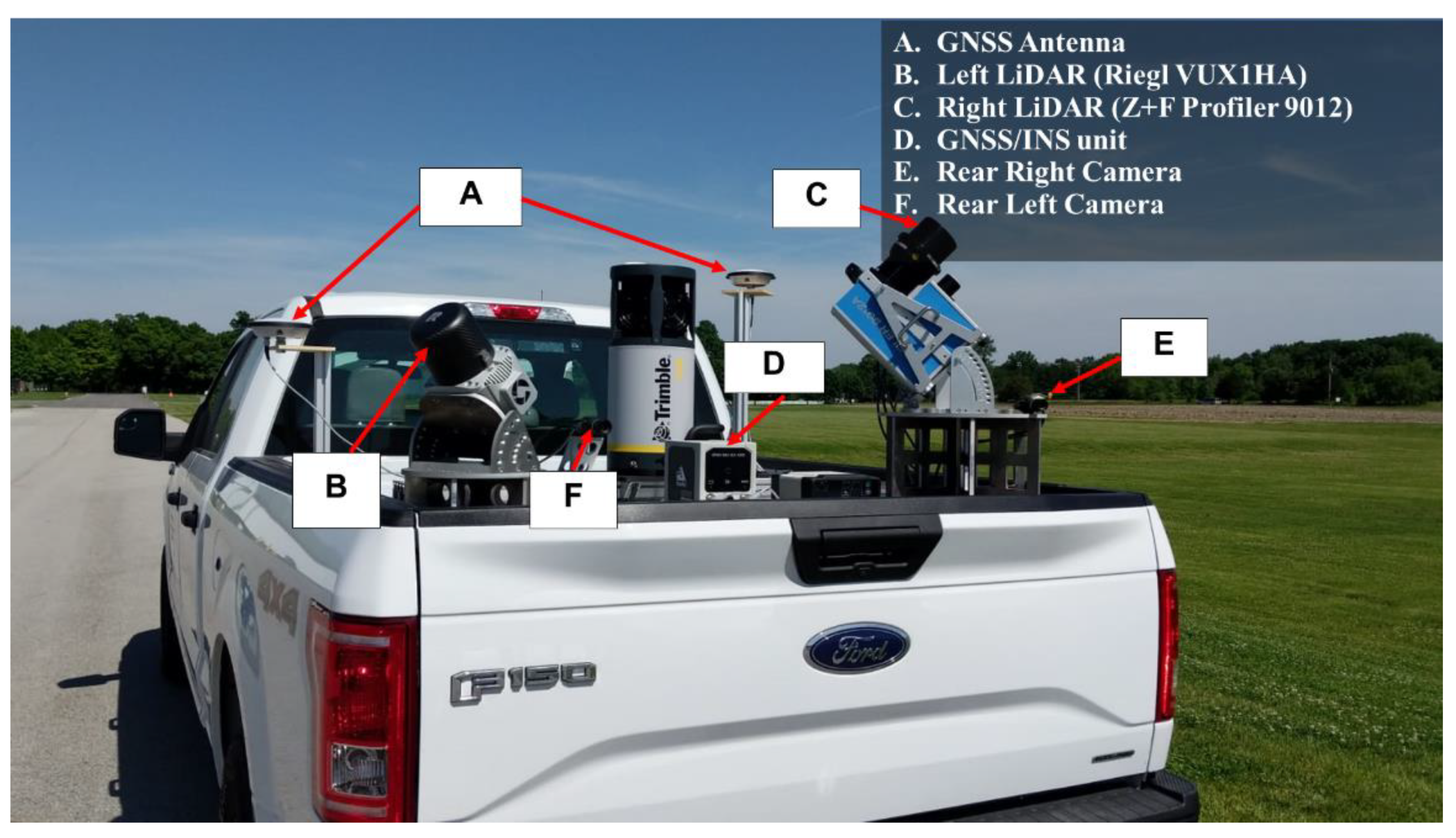
Remotesensing 12 00306 g004
Figure 5. Configuration of the wheel-based mobile LiDAR mapping system used for the acquisition of point clouds along MSE walls.
Remotesensing 12 00306 g005
Figure 6. Sample photos of the textured MSE walls at different sites (a) Site-1 and (b) Site-2 (the different tiles are highlighted by the red rectangles).
Remotesensing 12 00306 g006
Figure 7. Location and drive-run configuration for the dataset collection at (a) Site-1 and (b) Site-2.
Remotesensing 12 00306 g007
Figure 8. MSE wall point clouds collected by the MLS at (a) Site-1 and at (b) Site-2.
Remotesensing 12 00306 g008
Figure 9. Flowchart of the proposed methodology.
Remotesensing 12 00306 g009
Figure 10. Illustration of the Levelled Face coordinate system ( L F c s ) and Panel coordinate system ( P c s ).
Remotesensing 12 00306 g010
Figure 11. (a) Transformation from the source to the reference point cloud, and (b) conditions to accept the point-to-patch correspondence between the two point clouds.
Remotesensing 12 00306 g011
Figure 12. Point cloud registration of TLS dataset at Site-1 (colored by the RGB values from the TLS camera) and the MLS dataset (colored by intensity).
Remotesensing 12 00306 g012
Figure 13. An example of manual extraction of the faces along an MSE wall with piece-wise planar façade (different colors along the MSE wall represent the different registered scans).
Remotesensing 12 00306 g013
Figure 14. Normal distance map for a given face illustrating the fact that joints among the panels could be distinguished through their normal distance from the best fitting plane to that face (units for the values along the scale bar are in meters).
Remotesensing 12 00306 g014
Figure 15. An example of segmented textured MSE wall panels (different colors represent different segmented panels).
Remotesensing 12 00306 g015
Figure 16. Refined panel coordinate system (Pcs) through the estimated transformation parameters relating the template and matching panels.
Remotesensing 12 00306 g016
Figure 17. Longitudinal and transversal lines used to define the angular distortions for a planar face of the MSE wall at Site-1.
Remotesensing 12 00306 g017
Figure 18. Illustration of the relationship between L F c s and P c s for deriving the panel position and orientation serviceability measures.
Remotesensing 12 00306 g018
Figure 19. Evaluation of panel-to-panel out of-plane displacement.
Remotesensing 12 00306 g019
Figure 20. Cross sections illustrating the alignment quality of registered Riegl and ZF scans from a given drive run for the MSE wall at Site-1.
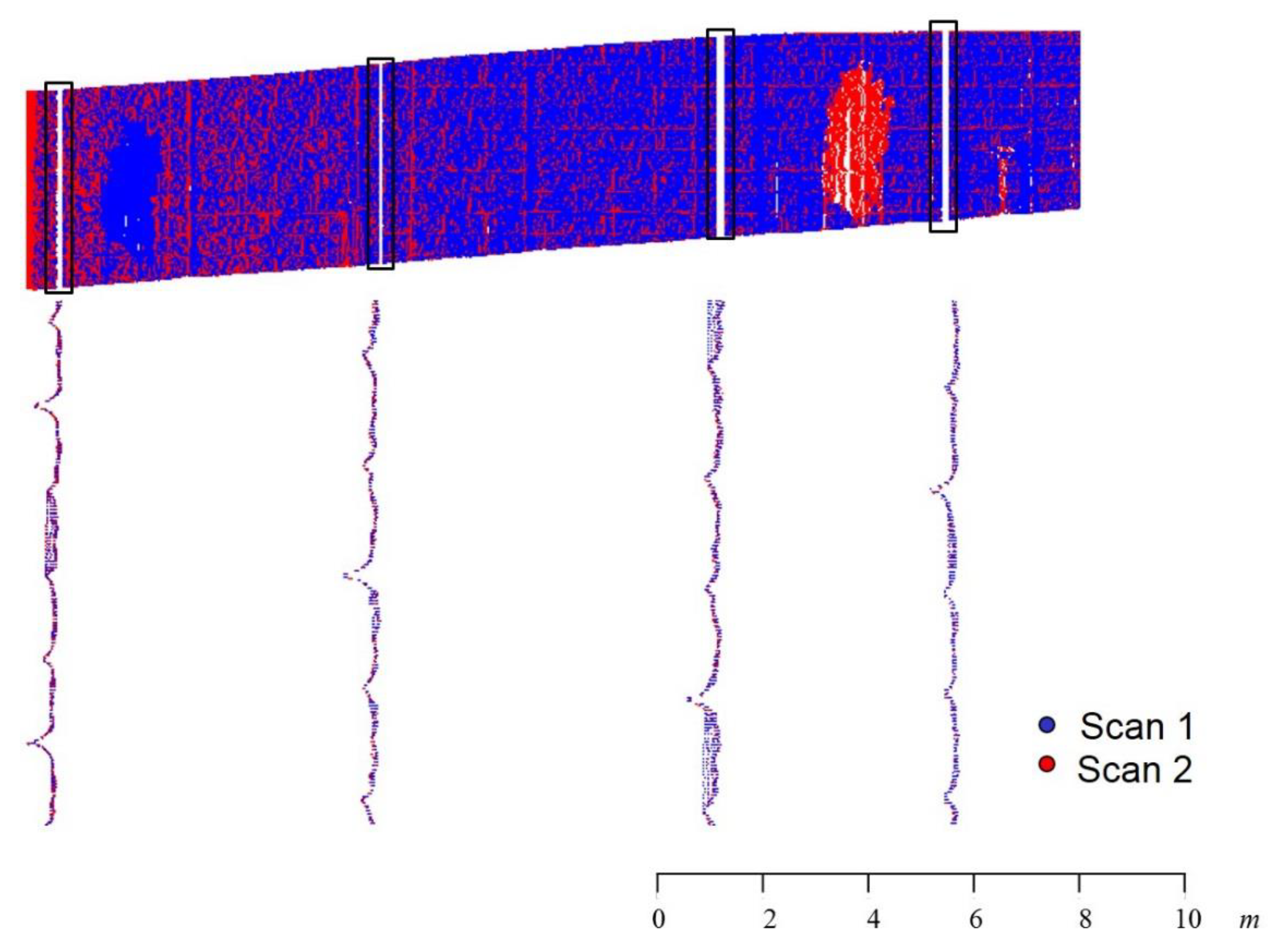
Remotesensing 12 00306 g020
Figure 21. Cross sections illustrating the alignment quality of registered point clouds from the two MLS drive runs for the MSE wall at Site-1.
Remotesensing 12 00306 g021
Figure 22. Cross sections illustrating the alignment quality of registered TLS scans of the MSE wall at Site-1.
Remotesensing 12 00306 g022
Figure 23. Cross sections illustrating the alignment quality of registered TLS and MLS point clouds for the MSE wall at Site-1.
Remotesensing 12 00306 g023
Figure 24. Angular distortion for the textured MSE wall face at Site-1: (a) longitudinal angular distortion along lines L1–L5, and (b) transversal angular distortion along lines T1-T12 (the horizontal lines represent the tolerable angular distortions)—L1–L5 and T1–T12 are illustrated in Figure 17.
Remotesensing 12 00306 g024
Figure 25. Cumulative Distribution Functions (CDF) for panel 3D orientation and panel-to-panel displacement using TLS (in blue) and MLS (in red) point clouds at Site-1.
Remotesensing 12 00306 g025
Figure 26. Cross sections illustrating the alignment quality of the Riegl and ZF point clouds from a given drive run of the MSE wall at Site-2.
Remotesensing 12 00306 g026
Figure 27. Cross sections illustrating the alignment quality of MLS point clouds from two drive runs in the same direction of the MSE wall at Site-2.
Remotesensing 12 00306 g027
Figure 28. Longitudinal and transversal lines used for defining angular distortions for one of the faces of the MSE wall at Site-2.
Remotesensing 12 00306 g028
Figure 29. Angular distortions for one of the faces of the MSE wall at Site-2: (a) longitudinal angular distortion along lines L1-L4, and (b) transversal angular distortion along lines T1-T9 (the horizontal red lines represent the tolerable angular distortions).
Remotesensing 12 00306 g029
Figure 30. Cumulative Distribution Functions (CDF) for the MLS-based panel 3D orientation and panel-to-panel displacement at Site-2.
Remotesensing 12 00306 g030
Table 1. Tolerable longitudinal angular distortion ( α L ) values for MSE walls constructed with incremental precast concrete panels (modified from [6]).
Joint Width wJ Panel Area ≤ 2.8 m2 (30 ft2)2.8 m2 (30 ft2) < Panel Area ≤ 7 m2 (75 ft2)
19 mm (0.75 inch)αL,tol = 1/100 = 0.01αL,tol = 1/200 = 0.005
13 mm (0.50 inch)αL,tol = 1/200 = 0.005αL,tol = 1/300 = 0.003
6 mm (0.25 inch)αL,tol = 1/300 = 0.003αL,tol = 1/600 = 0.002
Table 2. Estimated transformation parameters and quality measures (square root of a-posteriori variance factor, average normal distance among point-patch pairs, and RMSE of the normal distances) following the registration of the Riegl and ZF scans in a given drive run at Site-1.
XT (m ± mm)YT (m ± mm)ZT (m ± mm)Ω (deg ± sec)Φ (deg ± sec)Κ (deg ± sec) σ ° ^   ( m ) Average Normal Dist. (m)RMSE (m)
0.0200.0100.005−0.00120.0220.00030.00240.00230.0032
±0.01±0.03±0.02±0.003±0.029±0.004
Table 3. Estimated transformation parameters and quality measures (square root of a-posteriori variance factor, average normal distance among point-patch pairs, and RMSE of the normal distances) following the registration of the MLS point clouds from different drive runs at Site-1.
XT (m ± mm)YT (m ± mm)ZT (m ± mm)Ω (deg ± sec)Φ (deg ± sec)Κ (deg ± sec) σ ° ^   ( m ) Average Normal Dist. (m)RMSE (m)
−0.0580.0320.035−0.0120.1890.0090.0160.00980.018
±1.04±0.270±0.410±0.018±0.120±0.011
Table 4. Estimated transformation parameters and quality measures (square root of a-posteriori variance factor, average normal distance among point-patch pairs, and RMSE of the normal distances) following the registration of the TLS scans at Site-1.
XT (m ± mm)YT (m ± mm)ZT (m ± mm)Ω (deg ± sec)Φ (deg ± sec)Κ (deg ± sec) σ ° ^   ( m ) Average Normal Dist. (m)RMSE (m)
−0.81713.11−0.7220.040.011.060.0030.00480.005
±2.91±4.02±1.34±0.418±0.302±0.220
Table 5. Estimated transformation parameters and quality measures (square root of a-posteriori variance factor, average normal distance among point-patch pairs, and RMSE of the normal distances) following the registration of the MLS and TLS point clouds at Site-1.
XT (m ± mm)YT (m ± mm)ZT (m ± mm)Ω (deg ± sec)Φ (deg ± sec)Κ (deg ± sec) σ ° ^   ( m ) Average Normal Dist. (m)RMSE (m)
0.6410.431−0.181−0.0660.3411.670.0100.00520.008
±1.70±0.39±0.70±0.032±0.170±0.018
Table 6. TLS-based and MLS-based panel parametrization for the textured MSE wall at Site-1.
TLS-Based MeasuresMLS_Based Measures
IDXo (m)Yo (m)Zo (m) θ x p   ( deg ) θ y p   ( deg ) θ z p   ( deg ) Xo (m)Yo (m)Zo (m) θ x p (deg) θ y p (deg) θ z p (deg)
10.08−0.380.060.000.00−0.380.05−0.350.000.000.00−0.33
20.13−0.381.550.01−0.89−0.210.11−0.341.50−1.92−0.830.13
30.102.65−0.320.46−0.80−1.110.082.66−0.020.67−1.36−0.94
40.122.610.810.02−1.06−1.260.082.640.760.20−1.19−1.43
50.142.622.32−0.641.06−1.040.112.652.27−0.430.67−1.08
60.165.610.030.62−0.43−0.570.135.63−0.020.62−0.51−0.58
70.185.611.530.54−0.42−0.760.165.631.480.50−0.61−0.70
80.235.613.02−0.172.04−0.350.205.642.980.011.12−0.36
90.218.410.150.09−3.78−0.790.198.60−0.060.86−1.67−0.54
100.208.570.780.17−0.02−0.870.188.620.730.28−0.11−0.79
110.258.582.290.10−1.06−0.600.238.632.240.41−1.25−0.55
120.2511.580.400.34−0.88−0.420.2211.620.36−0.24−0.61−0.27
130.2711.571.520.21−0.43−0.080.2411.601.470.10−0.52−0.11
140.3011.583.020.34−1.05−0.070.2811.612.98−0.31−1.140.05
150.2714.560.770.46−0.620.050.2514.610.730.62−0.890.25
160.2914.562.280.37−1.24−0.060.2714.612.230.66−1.350.12
170.2914.583.770.300.000.010.2814.633.74−1.84−1.000.09
180.2817.560.760.92−1.440.210.2517.621.01−0.240.200.28
190.2817.561.540.24−0.59−0.080.2517.621.500.28−0.79−0.07
200.3017.563.040.30−1.19−0.060.2817.612.990.57−1.54−0.01
210.2720.551.111.54−0.420.300.2420.551.10−1.73−0.330.30
220.3020.552.280.01−0.710.260.2720.592.24−0.15−0.910.28
230.3120.553.78−0.65−1.680.100.2920.603.73−0.28−2.040.21
240.2823.551.530.37−1.41−0.060.2523.581.48−0.01−1.510.10
250.2823.553.020.48−1.11−0.200.2623.602.980.52−1.27−0.05
260.2526.511.520.37−0.440.480.2226.531.49−0.51−0.800.51
270.2726.532.280.32−0.810.630.2526.582.240.19−1.030.83
280.2926.543.770.490.150.610.2726.593.710.09−0.110.73
290.2229.671.900.280.010.130.2029.581.860.41−0.470.28
300.2629.533.040.28−0.660.450.2329.573.03−0.46−0.710.47
310.2332.522.290.37−0.861.230.2132.562.240.15−1.091.27
320.2632.523.780.54−0.631.410.2332.563.73−0.56−0.751.44
Table 7. TLS-based and MLS-based summary statistics of the derived serviceability measures for the MSE wall at Site-1.
TLSMLS
θ x p   ( deg ) θ y p   ( deg ) θ z p   ( deg ) Panel-to-Panel Displacement (mm) θ x p   ( deg ) θ y p   ( deg ) θ z p   ( deg ) Panel-to-Panel Displacement (mm)
Sample Size323232167323232169
Minimum Value−0.65−3.78−1.26−24.50−0.84−2.04−1.43−29.00
Maximum Value1.542.041.4123.100.861.121.4432.50
Range1.261.831.7447.601.391.871.9161.50
Average0.28−0.67−0.10−0.010.06−0.77−0.020.39
Standard Deviation0.390.920.628.280.460.670.638.59
5th Percentile−0.64−1.68−1.11−13.60−0.73−1.67−1.08−11.30
25th Percentile0.09−1.06−0.57−5.70−0.31−1.25−0.54−5.60
50th Percentile (median)0.30−0.71−0.070.200.09−0.890.040.10
75th Percentile0.46−0.420.215.400.41−0.510.285.50
95th Percentile0.620.150.6311.800.660.200.8313.50
Interquartile Range (IQR)0.370.640.7811.100.710.740.8211.10
Table 8. RMSE of the differences between the TLS-based and MLS-based serviceability measures for the MSE wall at Site-1.
Xo (m)Yo (m)Zo (m) θ x p   ( deg ) θ y p   ( deg ) θ z p (deg)Panel-to-Panel Displacement (m)
RMSE0.020.050.060.390.550.110.0178
Table 9. Estimated transformation parameters and quality measures (square root of a-posteriori variance factor, average normal distance among point-patch pairs, and RMSE of the normal distances) following the registration of the Riegl and ZF point clouds for one of the drive runs at Site-2.
XT (m ± mm)YT (m ± mm)ZT (m ± mm)Ω (deg ± sec)Φ (deg ± sec)Κ (deg ± sec) σ ° ^   ( m ) Average Normal Dist. (m)RMSE (m)
0.0110.0190.014−0.040.13−0.0080.00450.00330.0062
±0.02±0.04±0.03±0.011±0.029±0.004
Table 10. Estimated transformation parameters and quality measures (square root of a-posteriori variance factor, average normal distance among point-patch pairs, and RMSE of the normal distances) following the registration of the MLS point clouds from two drive runs of the MSE wall at Site-2.
XT (m ± mm)YT (m ± mm)ZT (m ± mm)Ω (deg ± sec)Φ (deg ± sec)Κ (deg ± sec) σ ° ^   ( m ) Average Normal Dist. (m)RMSE (m)
−0.065−0.009−0.037−0.011−0.0280.0090.00390.0030.0043
±0.01±0.02±0.02±0.007±0.014±0.00
Table 11. MLS-based panel parametrization for one of the MSE wall faces at Site-2.
IDXo (m)Yo (m)Zo (m) θ x p   ( deg ) θ y p   ( deg ) θ z p (deg)
10.020.060.130.000.000.96
20.030.050.800.712.520.92
30.080.052.34−0.122.011.12
40.120.003.87−1.113.451.15
5−0.023.050.09−0.151.800.29
60.003.061.540.882.620.24
70.053.053.11−0.291.450.20
8−0.046.050.12−0.260.670.58
9−0.036.030.810.032.810.48
100.026.042.35−0.082.790.30
110.066.023.82−0.481.020.30
12−0.059.160.51−0.331.31−0.04
13−0.039.031.531.023.25−0.31
140.059.053.09−0.540.970.19
15−0.0412.030.351.61−0.55−0.27
16−0.0412.050.84−0.233.06−0.29
170.0212.022.38−0.661.88−0.15
180.0412.043.89−0.221.760.14
19−0.0315.030.540.991.740.15
200.0115.031.61−0.282.400.34
210.0415.053.16−0.300.280.46
22−0.0418.030.800.452.13−0.24
230.0018.052.380.711.52−0.03
240.0218.023.820.331.090.05
25−0.0321.020.730.601.07−0.63
26−0.0221.031.551.273.07−0.99
270.0321.013.09−0.940.60−0.91
280.0320.964.64−1.930.83−0.32
290.0124.030.85−0.663.14−0.24
300.0724.022.35−0.521.07−0.23
310.0624.003.83−0.260.09−0.17
Table 12. MLS-based summary statistics of the serviceability measures for 285 panels of the MSE wall at Site-2.
θ x p   ( deg )
θ y p   ( deg )
θ z p   ( deg ) θ z p   ( deg )
Panel-to-Panel Displacement (mm)
Sample Size2852852851538
Minimum Value−2.95−2.09−1.72−31.40
Maximum Value2.853.611.8134.90
Range5.805.703.5366.30
Average0.160.550.01−0.21
Standard Deviation0.921.020.529.03
5th Percentile−1.10−0.87−0.86−14.70
25th Percentile−0.37−0.10−0.33−6.40
50th Percentile (median)0.000.410.00−0.30
75th Percentile0.731.120.345.90
95th Percentile1.892.620.8714.00
Interquartile Range (IQR)1.101.220.6712.30

