Performance Analysis of the Korean Positioning System Using Observation Simulation

Abstract

The Korean government has a plan to build a new regional satellite navigation system called the Korean Positioning System (KPS). The initial KPS constellation is designed to consist of seven satellites, which include three geostationary Earth orbit (GEO) satellites and four inclined geosynchronous orbit (IGSO) satellites. KPS will provide an independent positioning, navigation, and timing (PNT) service in the Asia-Oceania region and can also be compatible with GPS. In the simulation for KPS, we employ 24 GPS as designed initially and 7 KPS satellites. Compared to the true orbit that we simulated, the averaged root mean square (RMS) values of orbit-only signal-in-space ranging errors (SISRE) are approximately 4.3 and 3.9 cm for KPS GEO and IGSO. Two different positioning solutions are analyzed to demonstrate the KPS performance. KPS standard point positioning (SPP) errors in the service area are about 4.7, 3.9, and 7.1 m for east (E), north (N), and up (U) components, respectively. The combined KPS+GPS SPP accuracy can be improved by 25.0%, 31.8%, and 35.0% compared to GPS in E, N, and U components. The averaged position errors for KPS kinematic precise point positioning (KPPP) are less than 10 cm. In the fringe of the KPS service area, however, the position RMS errors can reach about 40 cm. Unlike KPS, GPS solutions show high positioning accuracy in the KPS service area. The combined KPS+GPS can be improved by 28.7%, 27.1%, and 30.5% compared to GPS in E, N, and U components, respectively. It is noted that KPS can provide better performance with GPS in the Asia-Oceania region.

1. Introduction

A global navigation satellite system (GNSS) refers to one or more satellite constellations providing a positioning, navigation, and timing (PNT) service to users around the world. GNSS is becoming an essential part of human life, which is used in many applications such as autonomous driving [1], surveying [2], precise time transfer [3], and mobile phones [4]. It even can contribute to many scientific fields [5,6,7,8].

GNSS includes the United States’ Global Positioning System (GPS), the Russian Federation’s GLObal NAvigation Satellite System (GLONASS), the European Union’s Galileo, and China’s BeiDou navigation satellite system (BDS). Each system comprises a constellation of satellites orbiting the Earth for different service purposes. The GPS consists of 31 medium Earth orbit (MEO) satellites in six equally spaced orbital planes with an inclination of approximately 55 degrees. GLONASS has 24 satellites in three orbital planes with an altitude of about 19,100 km and an inclination of 64.8 degrees. Galileo will consist of a total of 30 MEO satellites in three different orbital planes with an inclination of 56 degrees at an altitude of about 23,200 km, which is slightly higher than that for the GPS. The full operational capability (FOC) of Galileo is expected by the end of 2020 [9]. The Chinese BeiDou-3 was formally commissioned on 31 July 2020, making the completion of the “three-step” BDS development strategy. BeiDou-3 is composed of a constellation of 30 satellites, which include 24 in MEO, 3 in geostationary Earth orbit (GEO), and 3 in inclined geosynchronous orbit (IGSO) [10,11]. Including GEO and IGSO satellites is intended to provide regional navigation services [12].

There are also regional navigation satellite systems (RNSS) aiming to provide navigation services in a specific region. The representative systems as RNSS are the Indian “Navigation with Indian Constellation” (NAVIC) and Japanese “Quasi-Zenith Satellite System” (QZSS). NAVIC consists of seven satellites, which include three GEO satellites with an inclination of 5 degrees and four IGSO satellites every two in a different orbital plane. NAVIC is designed for providing navigation services in India. In addition, an area of 1500 km from the boundary of India is also covered by this system [9,13]. The QZSS satellite navigation system is compatible with GPS satellites [14]. It is designed so that at least one satellite is always visible over Japan. QZSS will consist of a total of seven satellites, which include four GEO and three IGSO satellites. The first QZSS satellite was launched in 2010, and three QZSS satellites were launched in 2017. The QZSS has a plan to provide a highly precise positioning service for users in Japan with a high elevation angle to improve the signal reception, and its service area will also cover the East Asia and Oceania region [15].

In the process of preparing for the development of a new GNSS system, its performance can be predicted through various simulations. Wu et al. [16] presented simulation results for the performance of GPS augmentation using QZSS in specific areas. Ge et al. [17] investigated the availability of a low Earth orbit (LEO) constellation transmitting navigation signals for a positioning service. From the simulation results, they showed that the LEO constellation can contribute to improving the performance of GNSS precise point positioning (PPP). Multi-constellation positioning with an increased number of navigation satellites can significantly improve the accuracy and precision of positioning. Li et al. [18] investigated that the LEO constellation can significantly enhance the performance of current multi-GNSS real-time PPP using simulated data. Their results also demonstrated that the LEO-enhanced GNSS can be beneficial for precise positioning. The accuracy of GNSS PPP depends on the quality of GNSS orbits and clock products. Some studies investigated improving the orbit quality of new GNSS satellites, such as Galileo and BDS [19,20].

Recently, the Korean government has proposed to build a new RNSS system [9], which is called the Korean Positioning System (KPS). It is planned for full operational capability in 2039. The initial KPS constellations are composed of seven satellites, which include three GEO and four IGSO satellites. KPS will provide independent navigation services in its service area. However, it can be compatible with GPS as a regional augmentation system. This is also why the GPS constellation will be included in this study.

In this study, we briefly introduce the KPS system with its configuration. As there are no KPS observations at ground stations, we simulate all observations. For its performance evaluation, we employ 24 GPS as designed initially and 7 KPS satellites planned for the PNT services in the Asia-Oceania region. Preliminary results related to the KPS performance are analyzed with simulated observations, which include the number of visible satellites for availability, precise orbit determination (POD), signal-in-space ranging errors (SISRE), standard point positioning (SPP), and kinematic PPP (KPPP). This study also includes an analysis of the expected accuracies that is carried out when using this system with GPS.

2. KPS and GPS Constellations

The constellation configuration of KPS is proposed to provide continuous satellite navigation services in regional coverages, including East Asia and Oceania. The initial constellation of KPS comprises seven satellites of two different orbit types. The three GEO satellites have a semi-major axis of about 42,164 km and have the same orbital period as Earth’s rotation period. They are deployed on Earth’s equator with an inclination of 0 degrees at about 78°E, 128°E, and 178°E, respectively. The four IGSO satellites in the constellation have the same orbital period and semi-major axis as GEO satellites. They are centered at 128°E (i.e., equator crossing point) with a nominal 90 degrees separation in the argument of latitude and right ascension of the ascending node (RAAN). They also have an inclination of 43° and an eccentricity of about 0.075. In addition, KPS IGSO satellites have different orbital planes, but all have the same ground track repeating daily.

The GPS satellites in the constellation for orbit simulations are deployed in six equally spaced orbital planes. GPS consists of 24 MEO satellites with four satellites in each plane. The MEO satellites have circular orbits with an eccentricity of zero, a semi-major of 26,587 km, and an inclination of 55° with an altitude of 20,200 km [21]. The orbital period for GPS MEO satellites is precisely half a sidereal day (~11 h 58 m).

In this study, we first consider the orbit simulation with 24 GPS and 7 KPS satellites.

Table 1. The orbit parameters and designed constellations for the Global Positioning System (GPS) [21] and Korean Positioning System (KPS).

GNSS Parameter		GNSS System
	GPS	KPS
Orbit type	MEO	GEO	IGSO
Number of satellites	24	3	4
Semi-major axis	26,587 km	42,164 km	42,164 km
Inclination	55°	0°	43°
Eccentricity	0	0	0.075
Constellation	Four satellites in 6 orbital planes	78°E, 128°E, 178°E	RAAN ~ 218°, 128°, 38°, 308°

lists the orbit parameters and designed constellations for GPS and KPS satellites. It includes the number of satellites, semi-major axis, inclination, eccentricity, and distribution of the three different orbit types.

3. Simulations

3.1. Observation Simulation

Since KPS is a planned regional satellite navigation system, there are no actual data. Therefore, a software package for observation simulation is essential to analyze the performance of KPS. In this study, we adopted the simulation package in the Positioning and Navigation Data Analyst (PANDA) software developed by Ge [17] for KPS/GPS simulation and orbit and clock determination, as well as the PPP package developed by Liu and Ge [22] for KPS/GPS validation. It is assumed that KPS uses the same frequency as GPS. The GPS correction and observation models are applied directly to KPS.

The observation equations for dual-frequency measurements can be expressed as follows [23]:

$$P_1^{sys}=\rho +c·\left(d{t}_r-d{t}^s\right)+I_1+T+{\epsilon }_{P_1}$$

(1)

$$P_2^{sys}=\rho +c·\left(d{t}_r-d{t}^s\right)+\frac{f_1^2}{f_2^2}{I}_1+T+{\epsilon }_{P_2}$$

(2)

$$L_1^{sys}=\rho +c·\left(d{t}_r-d{t}^s\right)-I_1+T+{\lambda }_1{N}_1+{\epsilon }_{L_1}$$

(3)

$$L_2^{sys}=\rho +c·\left(d{t}_r-d{t}^s\right)-\frac{f_1^2}{f_2^2}{I}_1+T+{\lambda }_2{N}_2+{\epsilon }_{L_2}$$

(4)

where $P$ and $L$ represent the code and carrier-phase measurements, respectively. The superscript $sys$ indicates the GPS or KPS system, and the subscripts 1 and 2 indicate the frequency. $\rho$ is the distance, including the geometric distance from the satellite to the ground receiver, antenna phase center offsets (PCO), and phase center variations (PCV) of the satellites and receivers, the relativistic correction, and tidal effects. $c$ represents the speed of light in a vacuum. $d{t}_r$ and $d{t}^s$ denote the satellite and receiver clock errors that are estimated as white noise. $I_1$ is the ionospheric delay, and $T$ represents the tropospheric delay. $N$ is the integer ambiguity parameter. ${\epsilon }_P$ and ${\epsilon }_L$ denote the code and carrier-phase observation noise, which have a standard deviation of 1.0 and 0.005 m with zero-mean Gaussian distribution. They are somehow simplified since the observation noise is usually elevation-dependent. In the data processing stage, we use the elevation weights, not the equal weights for observations. $f_1$ and $f_2$ are the frequencies for L1 and L2 signals. ${\lambda }_1$ and ${\lambda }_2$ are the wavelengths for L1 and L2 signals.

The International GNSS Service (IGS) provides the absolute antenna phase center correction model, including the PCO and PCV [24]. The PCO and PCV corrections for GPS satellites from the igs14.atx are applied for observation simulation, while those for KPS satellites are assumed to be zero. The PCO and PCV corrections are dependent on the GNSS signal frequencies. In this study, those for ground receivers are assumed as the same value as the GPS signal frequencies. Moreover, the white noise model was applied for simulation of the KPS/GPS satellite and receiver clock offsets. The tropospheric delay is still a significant error source in GNSS precise positioning. The tropospheric delays at ground stations are corrected by the a priori Saastamoinen model [25] and the global mapping function [26].

SPP is considered for positioning performance of single-frequency users and is referred to as single point positioning using pseudo-range measurements and navigation parameters. For KPS/GPS SPP simulation, we use only the simulated P1 code measurements, as presented in Equation (1). The error sources in SPP simulation include satellite ephemeris, satellite clock, atmospheric effects (ionosphere and troposphere), and observation noises. In this study, precise satellite orbit and clock products generated by orbit simulations are considered for KPS/GPS SPP.

A kinematic PPP is also adopted to investigate the performance of precise positioning for the simulated KPS and GPS observations in the regional service area. In general, GNSS PPP uses dual-frequency measurements to obtain a precise position solution with a single station only [27]. To remove the first-order ionospheric delay, the linearized observation equations for the ionosphere-free (IF) code and phase linear combinations can be written as follows [27]:

$$P_{IF}=\rho +c·\left(d{t}_r-d{t}^s\right)+T+{\epsilon }_{P_{IF}}$$

(5)

$${\mathsf{\Phi }}_{IF}=\rho +c·\left(d{t}_r-d{t}^s\right)+T+N_{IF}+{\epsilon }_{{\mathsf{\Phi }}_{IF}}$$

(6)

where $P_{IF}$ and ${\mathsf{\Phi }}_{IF}$ are the IF code observables and IF phase observables, respectively. $\rho$ is the geometric range from the GNSS satellite to the ground receiver, and $c$ is the speed of light. $N_{IF}$ is the IF phase ambiguity. ${\epsilon }_{P_{IF}}$ and ${\epsilon }_{{\mathsf{\Phi }}_{IF}}$ represent the code and phase measurement noises by IF combinations, respectively.

3.2. Precise Orbit Simulation

In this study, we first evaluate KPS and GPS POD performance with simulated data on the PANDA software. To investigate the performance of KPS/GPS POD, we also consider 11 temporary KPS monitoring stations (KPSMS) and 10 additional Multi-GNSS Experiment (MGEX) stations to simulate ground-based observations for three days, doy 140–142, 2018. The sampling intervals of the simulated observations are set to 30 s for ground stations. Figure 1 shows the distribution of KPSMS and MGEX stations selected temporarily for the KPS/GPS POD simulations. The filled blue circles and red triangles represent the MGEX and KPSMS stations, respectively.

In batch least squares (LSQ) mode, we use 24 h data for one POD solution. In the solution, the ionospheric free linear combinations are used to eliminate the first-order ionospheric delay, and the unknown parameters to be estimated include initial position and velocity, solar radiation parameters, the satellite clock offsets, station coordinates, which are usually tightly constrained though they are estimated as parameters, receiver clock offsets, integer ambiguities, and zenith wet delays (ZWD).

Table 2. Force and observation models applied for the KPS/GPS POD simulation.

Item	Models/Methods
Force model
Earth gravity	EIGEN6C (12 × 12) [29]
N-body	JPL DE405 [30]
Relativity	IERS conventions 2010 [31]
Solar radiation pressure	ECOM model [32]
Atmospheric drag	Not considered
Earth orientation	IERS C04 [33]
Attitude model	Orbit normal [34] for KPS GEO, yaw steering and orbit normal for KPS IGSO and GPS
Observation model
Observations	Undifferenced ionospheric free linear combination
Signal	L1/L2
Elevation cutoff	7°
Weight for observations	Elevation ($E$)-dependent angle stochastic model (${\sigma }^2=1$ for $E$ > 30°, otherwise ${\sigma }^2=1/2\sin \left(E\right))$
Sampling rate	30 s
Arc length	1 day
Reference frame	ITRF2014
Satellite PCO/PCV	Igs14.atx
Receiver PCO/PCV	Igs14.atx
Phase wind-up	Wu et al. [35]
Solid earth tide, ocean tide, pole tide	IERS conventions 2010 [31]
Ionospheric delay	Eliminated
Tropospheric delay	Saastamoinen with GMF [26], estimated zenith wet delay
Satellite clock error	Estimated as white noise
Receiver clock error	Estimated as white noise
Ambiguity	Fixed solutions

presents the force and observation models applied for KPS/GPS POD simulation. Figure 2 shows the ground tracks of KPS and GPS satellites. KPS IGSO satellites have repeating analemma ground tracks with north-south asymmetry. This is very similar to the ground tracks of QZSS IGSO satellites. KPS GEO satellites are placed at regular intervals near the Earth’s equator. In addition, the ground tracks for 24 GPS satellites are marked with solid green lines, as shown in Figure 2.

Figure 3 presents the averaged orbit root mean square (RMS) errors in the along-track, cross-track, and radial directions for seven KPS satellites. The orbit errors of all components were compared with the true orbits that we have simulated. For the KPS GEO satellites (PRN K01 ~ K03) in regional coverage, it is feasible to obtain the orbit accuracy in terms of three dimensional RMS at about 50 cm, while the orbit accuracy of the KPS IGSO satellites (PRN K04 ~ K07) to be achieved is about 10 cm. As seen in Figure 3, the RMS values of the GEO satellites are much larger in the along-track direction than in the others. In addition, the RMS of the POD solution for KPS GEO satellites is less than 10 cm in the cross-track and radial directions. The averaged RMS values in the radial direction are the smallest, while the averaged RMS value in the along-track direction reaches up to nearly 50 cm. Geng et al. [36] reported that the weak tracking geometry of GEO satellites results in large orbit errors in the along-track directions. Moreover, Ge et al. [37] indicated that the orbit errors of GEO satellites in the along-track are highly correlated with the ambiguity solutions. Xu et al. [38] showed that the RMS value in the along-track direction is about 46–73 cm for BDS GEO satellites with ground tracking observations only. In addition, the RMS values in all directions for BDS IGSO satellites were less than 20 cm. Although KPS and BDS differ slightly in the designed orbital elements, the KPS orbit simulation results are very similar to those presented by Xu et al. [38]. Therefore, it is possible to predict the performance of KPS POD by orbit simulations.

Figure 4 shows the averaged orbit RMS errors in the along-track, cross-track, and radial directions for 24 GPS satellites. These errors were compared with the true orbits that we simulated. The orbit accuracy of the GPS satellites is less than 5 cm in all directions. The GPS satellites exhibit higher orbit accuracy in all directions than the KPS satellites. In general, while the GEO and IGSO satellites have limited coverage, MEO satellites like GPS provide global coverage. This indicates that GPS has much better observation geometry compared to KPS. Li et al. [39] suggested that the quality of GEO orbits can be improved by LEO satellites. However, KPS does not consider LEOs.

As shown in Figure 4, the averaged RMS value of the along-track component is larger than that of the others, whereas the radial component of GPS has slightly better accuracy than the along-track and cross-track components.

IGS has provided orbit products for GPS satellites [24]. The IGS final products have a nominal orbit accuracy of about 2.5 cm [40], which are available at the website (http://www.igs.org/products). Our results derived from simulations are similar to those provided by IGS.

4. Performance Analysis for KPS

4.1. Satellite Visibility

As one of the critical indicators for the system performance, we considered the number of visible satellites. To compare the average number of visible satellites on global coverage, the computations were performed for two different constellation combinations (KPS-only and KPS+GPS). The elevation cutoff angle of satellites is set to 10°. The coordinate grids have a spatial resolution with 2.5° in latitude and 5° in longitude. Consequently, we calculate the average number of visible satellites at each grid point.

Figure 5 shows the average number of visible satellites on a global scale for KPS-only, KPS-only ($\ge$4 SV), and KPS+GPS, respectively. As shown in Figure 5a, KPS satellites aim to provide its services in the Asia-Oceania region. The area that can receive all seven KPS satellites is located between 35°S and 35°N latitude and 90°E and 162°E longitude. In addition, the area plotted in Figure 5b can track more than four KPS satellites. The positioning service for KPS is available only in this area. The combination of KPS and GPS can utilize the signals of many satellites in the Asia-Oceania region. In such areas, the maximum number of visible satellites is 16. The minimum number of visible satellites on average is 10.

4.2. Signal-In-Space Ranging Error

To comprehensively assess the accuracy of the simulated KPS and GPS precise orbits, SISRE values for KPS and GPS are analyzed. SISRE is one of the key indicators for evaluating the performance of a GNSS system [41,42]. The SISRE can be expressed as Equation (7).

$$\mathrm{SISRE}=\sqrt{w_R^2·R^2+w_{A,C}^2·\left(A^2+C^2\right)}$$

(7)

where $w_R^2$ and $w_{A,C}^2$ are the weight factors of orbit errors for radial ($R)$, along-track ($A)$, and cross-track ($C)$, respectively. $w_R^2$ and $w_{A,C}^2$ are 0.99 and $\raisebox{1ex}{$1$}\!\left/ \!\raisebox{-1ex}{$127$}\right.$ for KPS IGSO and GEO satellites, 0.98 and $\raisebox{1ex}{$1$}\!\left/ \!\raisebox{-1ex}{$54$}\right.$ for GPS satellites [43]. The SISRE is computed as the RMS value of the orbital accuracy. It is also determined as the relative weight of each orbital error. The smaller the SISRE, the better the performance of the system.

Figure 6 presents the orbit-only SISRE for KPS satellites with an additional division to GEO and IGSO satellites. The blue and orange vertical bars represent SISRE values for KPS GEO and KPS IGSO satellites, respectively. The RMS values of SISRE range from 2 to 6 cm. The SISRE values for KPS IGSO are slightly smaller than those for KPS GEO. The averaged RMS values of SISRE are approximately 4.3 and 3.9 cm for KPS GEO and KPS IGSO, respectively. An SISRE value from real-time GNSS data via Internet streams was reported by Kazmerski et al. [44]. They showed that the averaged RMS values of SISRE are approximately 12.3 and 11.1 cm for BeiDou GEO and BeiDou IGSO, respectively. The SISRE of KPS is about three times smaller than that of BeiDou. However, it is still worse compared to GPS (~1.2 cm). Therefore, it can be attributed to the difference in orbital errors between KPS and BeiDou. Since the SISRE for KPS is computed by observation simulation, it may differ from real values. In addition, the SISRE values for some KPS satellites significantly differ from the averaged value, as shown in Figure 6.

Figure 7 presents the orbit-only SISRE for each GPS satellite. The RMS values of the SISRE for GPS are at the level of a few centimeters. The averaged RMS value of the SISRE is approximately 1.2 cm for GPS. As shown in Figure 4, GPS orbit accuracy calculated by the orbit simulation was at the level of 2–5 cm. Therefore, SISRE values for GPS reflect the corresponding orbit accuracy. Zhang et al. [45] showed that the orbit-only SISRE for each GPS satellite is achieved at a level of 5 cm using the MADOCA real-time products. Therefore, it can be seen that the SISRE calculated by simulated orbits has little difference compared to the real orbit products. Moreover, the orbit-only SISRE can be influenced by different distributions of ground reference stations.

4.3. Standard Point Positioning (SPP)

The SPP mode has been widely used for most navigation users. It is referred to as absolute positioning, which employs the L1 code measurements with the broadcast satellite orbit and clock error information to calculate a position for the user. Its positioning accuracy can be achieved at a level of a few meters [46]. In this study, the positioning performance for KPS single-frequency users was analyzed. 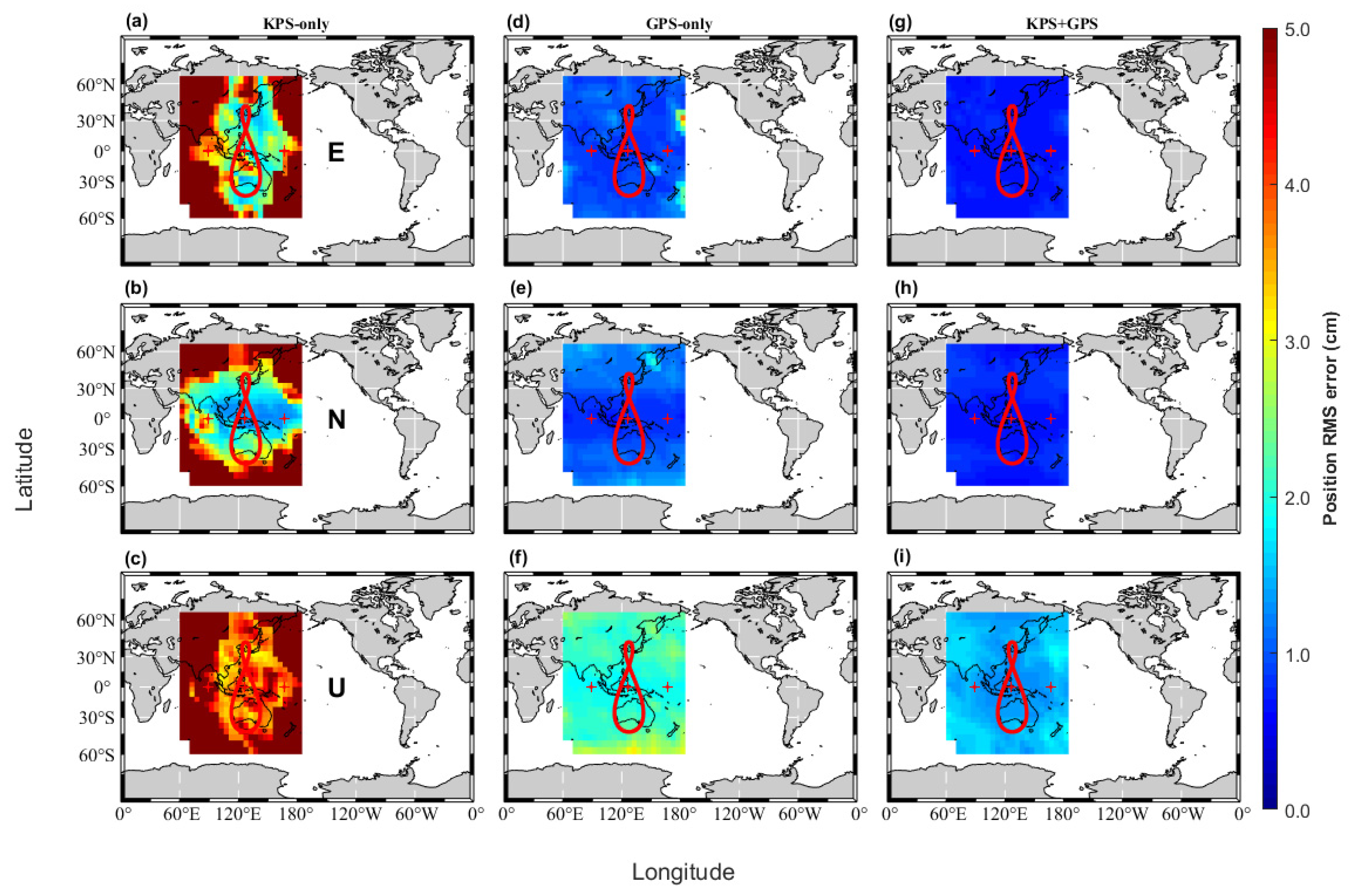Figure 8 shows the positioning accuracies for KPS-only, GPS-only, and KPS+GPS in the east (E), north (N), and up (U) components, respectively. We mainly considered SPP performance for KPS and GPS on a regional scale. For SPP, we also set the regular grids with the area that covers from 60°S to 60°N latitude and 60°E to 180°E longitude. The grid points are evenly spaced in latitude and longitude. As such, we process simulated observations for SPP at the grid points with a spatial resolution of 5° by 5° on a regional scale. The E component for KPS has the smallest RMS value at the central longitude of 128°E. The performance of SPP tends to drop sharply away from the central longitude of KPS IGSO satellites. It is directly related to the average number of visible satellites on the ground stations. When the number of visible satellites is less than 5, the KPS can result in large positioning errors of more than a few tens of meters. The N component has a small RMS value near the earth equator and has a large RMS value at higher latitude regions. An error of the U component is very similar to that of the E one. The KPS presents a good performance in the horizontal components. However, the RMS values of the vertical component are relatively large compared to those of the horizontal components.

GPS has better SPP performance on a regional scale compared to KPS. GPS also provides consistent SPP performance at all grid points on a regional scale. In addition, the RMS value of U components is relatively large compared to the E and N components. The combined KPS and GPS SPP solutions are shown in the right Figure 8g–i. Obviously, combined KPS and GPS presents the highest positioning accuracy for all three components on a regional scale. It is noted that the combination of KPS and GPS can significantly improve the SPP performance.

For each station, the RMS values for SPP errors are plotted in the E, N, and U components using a histogram. Furthermore, histograms are calculated by a 95% confidence level with the normal approximation. Figure 9 is related to the grids in Figure 8. It shows the probability distributions of the SPP position RMS errors in each component for KPS, GPS, and combined KPS+GPS, respectively. For statistical analysis, we investigated the averaged RMS values in each component. As shown in Figure 9, the averaged RMS values on a regional scale for KPS are about 4.7, 3.7, and 7.1 m for E, N, and U components, respectively. For GPS, the averaged value is about 1.2, 1.4, and 3.1 m for each component, respectively. It can be seen that the SPP performance of KPS is relatively poor compared to GPS. The positioning errors for KPS in each component are approximately twice those of GPS with respect to SPP on a regional scale. In particular, the error of the vertical component is relatively large compared to the horizontal components. While the position errors of the horizontal components are distributed less than about 1.2 cm, the vertical component is concentrated from about 1.5 to 3.0 cm. As shown in the right Figure 9g–i, the combination of KPS and GPS gives better positioning performance compared to KPS and GPS. The averaged RMS values for combined KPS+GPS are about 0.9, 0.9, and 2.0 m for E, N, and U components, respectively. Furthermore, the positioning accuracy for the combined KPS+GPS was improved by 25.0%, 31.8%, and 35.0% in each component compared to that for GPS.

4.4. Precise Point Positioning (PPP)

To show the feasibility of precise positioning on a regional scale for KPS, we examine the performance of different kinematic PPP (KPPP) processing. Figure 10 shows the KPPP positioning accuracy for KPS, GPS, and combined KPS+GPS in the E, N, and U components, respectively. KPS is not available anywhere globally. As clearly shown in Figure 10, the KPS service area is limited only to the East Asia and Oceania regions. KPS KPPP results are very similar to KPS SPP in terms of the characteristics of the positioning errors. As with KPS SPP, the positioning accuracy is relatively high in areas where five or more visible satellite signals on the ground can be tracked. The positioning accuracy of KPS tends to drop sharply with the average number of visible satellites on a regional scale.

The positioning accuracy of KPPP is very different from that of SPP. While SPP has meter-level positioning accuracy, KPPP can achieve centimeter-level solutions. As shown in the middle Figure 10d–f, GPS solutions provide stable positioning performance in the regional area. Compared to KPS and GPS, combined KPS+GPS can improve the positioning accuracy significantly. In the KPS service area, it can be seen that the combined KPS+GPS solutions can achieve position accuracy of less than about 1 and 2 cm in the horizontal and vertical components, respectively.

For the numerical analysis of KPPP results, we present the probability distribution for the corresponding position RMS errors. Figure 11 is related to the grids in Figure 10. The RMS errors at the grid points are expressed as the probability distributions for KPS, GPS, and KPS+GPS KPPP. The averaged values of position errors for KPS are approximately 7.5, 5.8, and 9.1 cm in the E, N, and U components, respectively. The averaged position errors in all three coordinate components were lower than 10 cm. In the fringe of the KPS service area, however, KPS errors can reach to about 40 cm. This indicates that the number of visible satellites can result in large positioning errors in KPPP mode.

As shown in the middle Figure 11d–f, GPS is more accurate than KPS. The absolute accuracy of GPS in all components is within a range of 0 to 4 cm. The position errors on average are about 1.0, 1.0, and 2.1 cm in each component, respectively. Moreover, the vertical component for GPS is statistically concentrated on the positioning errors between 1.8 to 3.0 cm. The vertical error is related to the satellite geometry. It is relatively larger than the horizontal one.

The positioning accuracy of the combined KPS+GPS was significantly improved compared to KPS and GPS. The averaged position errors were about 0.7, 0.8, and 1.5 cm in each component, respectively. In the KPPP mode, the integration of KPS and GPS can provide higher accuracy, which can be better than 1 and 2 cm for the horizontal and vertical components, respectively. For the bulk of the positioning errors less than 1 cm, the E and N components provide similar performance. Furthermore, the U component presents a large population of positioning errors between 1.2 and 2.0 cm. The positioning accuracy for the combined KPS+GPS was improved compared to GPS by approximately 28.7$\%$, 27.1$\%$, and 30.5% in each component.

In this study, the combined KPS+GPS improved the position accuracy in both SPP and KPPP modes compared to KPS and GPS. As a result, it is noted that KPS with GPS can contribute to the improvement of the positioning accuracy.

5. Summary and Conclusions

In this study, we presented the initial KPS constellation. We also performed simulations to investigate the performance of the designed KPS in the service area. For KPS GEO satellites, the achievable orbit precision with the simulated ground data was approximately 50 cm 3-d RMS compared to the true orbit that we simulated, while KPS IGSO POD was approximately 10 cm. Moreover, the performance indicators for KPS/GPS were analyzed in terms of satellite visibility, SISRE, SPP, and KPPP.

The area where seven KPS satellite signals are tracked on the ground at the same time is located at 35° S–35° N latitude and 90° E–162° E longitude.

With the simulated precise KPS/GPS orbit products, we calculated the orbit-only SISRE for KPS/GPS. The averaged RMS values of the orbit-only SISRE were approximately 4.3 cm for KPS GEO and approximately 3.9 cm for KPS IGSO. The SISRE of KPS IGSO was slightly smaller than that of KPS GEO. However, the SISRE of KPS was relatively large compared to that of GPS. It is directly related to the KPS orbit accuracy.

The performance of KPS SPP tends to decrease sharply as the distance from the central longitude of IGSO satellites increases. It is directly related to the average number of visible satellites on the ground stations. In addition, the KPS SPP can result in large positioning errors of tens of meters when the number of visible satellites is less than five. The positioning errors for KPS SPP in the service area were about 4.7, 3.9, and 7.1 m for the E, N, and U components, respectively. For the GPS SPP solution, they were about 1.2, 1.4, and 3.1 m for each component. Therefore, it can be seen that the KPS-only SPP derived from the simulation has a poor performance in positioning accuracy compared to the GPS-only SPP. Furthermore, we showed that the combination of KPS and GPS can significantly improve the positioning performance.

The averaged position errors for the KPS-only KPPP in the service area were less than 10 cm. This indicates that the KPS system can have the capability of precise positioning. In some regions, the errors of the KPS-only KPPP reached about 40 cm. Unlike KPS, the GPS-only KPPP solutions showed high positioning accuracy in the KPS service area. In addition, the positioning accuracy in the KPPP mode was further improved by combining KPS and GPS. With the comprehensive performance of KPS from the simulation, KPS can provide better performance with GPS in the Asia-Oceania region.

As a result, we presented some predicted performances, including different positioning results in future KPS operating modes. The KPS system is expected to be valuable and contribute to GNSS users.

References

- Zein, Y.; Darwiche, M.; Mokhiamar, O. GPS tracking system for autonomous vehicles. Alex. Eng. J. 2018, 57, 3127–3137. [Google Scholar] [CrossRef]
- Bakula, M. An approach to reliable rapid static GNSS surveying. Survey Rev. 2012, 44, 265–271. [Google Scholar] [CrossRef]
- Tavella, P.; Petit, G. Precise time scales and navigation systems: Mutual benefits of timekeeping and positioning. Satell. Navi. 2020, 1, 1–10. [Google Scholar] [CrossRef]
- Dabove, P.; Pietra, V.D.; Piras, M. GNSS Positioning Using Mobile Devices with the Android Operating System. Int. J. Geo Inf. 2020, 9, 220. [Google Scholar] [CrossRef] [Green Version]
- Bevis, M.; Businger, S.; Herring, T.A.; Rocken, C.; Anthes, R.A. GPS meteorology: Remote sensing of atmospheric water vapor using GPS. J. Geophys. Res. 1992, 97, 787–801. [Google Scholar] [CrossRef]
- Hernández-Pajares, M.; Juan, J.M.; Sanz, J. High resolution TEC monitoring method using permanent ground GPS receivers. Geophys. Res. Lett. 1997, 24, 1643–1646. [Google Scholar] [CrossRef] [Green Version]
- Kato, T.; Terada, Y.; Kinoshita, M.; Kakimoto, H.; Isshiki, H.; Matsuishi, M.; Yokoyama, A.; Tanno, T. Real-time observation of tsunami by RTK-GPS. Earth Planets Space 2000, 52, 841–845. [Google Scholar] [CrossRef] [Green Version]
- Larson, K.M. GPS seismology. J. Geod. 2009, 83, 227–233. [Google Scholar] [CrossRef]
- Hein, G.W. Status, perspectives and trends of satellite navigation. Satell. Navi. 2020, 1, 11–22. [Google Scholar] [CrossRef]
- CSNO. Beidou Navigation Satellite System Signal in Space Interface Control Document Open Service Signal (Version 2.1). Available online: http://www.beidou.gov.cn/xt/gfxz/201710/P020171202693088949056.pdf (accessed on 12 September 2017).
- CSNO. Beidou Navigation Satellite System Signal in Space Interface Control Document Open Service Signal B2b (Version 1.0). Available online: http://en.beidou.gov.cn/SYSTEMS/Officialdocument/202008/P020200803544811195696.pdf (accessed on 3 August 2020).
- Yang, Y. Progress, contribution and challenges of compass/Beidou satellite navigation system. Acta Geod. Cartogr. Sin. 2010, 39, 1–6. [Google Scholar]
- Zaminpardaz, S.; Teunissen, P.J.G.; Nadarajah, N. IRNSS/NavIC and GPS: A Single and Dual System L5 Analysis. J. Geod. 2017, 91, 915–931. [Google Scholar] [CrossRef] [Green Version]
- Safoora, Z.P.; Kan, W.; Peter, J.G. Teunissen. Australia-first high-precision positioning results with new Japanese QZSS regional satellite system. GPS Solut. 2018, 22, 101. [Google Scholar] [CrossRef] [Green Version]
- Ye, H.; Jing, X.; Liu, L.; Wang, M.; Hao, S.; Lang, X.; Yu, B. Analysis of Quasi-Zenith Satellite System Signal Acquisition and Multiplexing Characteristics in China Area. Sensors 2020, 20, 1547. [Google Scholar] [CrossRef] [Green Version]
- Wu, F.; Kubo, N.; Yasuda, A. Performance Evaluation of GPS Augmentation using Quasi-Zenith Satellite System. IEEE Trans. Aero. Elec. Syst. 2004, 40, 1249–1260. [Google Scholar] [CrossRef]
- Ge, H.; LI, B.; Ge, M.; Zang, N.; Nie, L.; Shen, Y.; Schuh, H. Initial Assessment of Precise Point Positioning with LEO Enhanced Global Navigation Satellite Systems (LeGNSS). Remote Sens. 2018, 10, 984. [Google Scholar] [CrossRef] [Green Version]
- Li, B.; Ge, H.; Ge, M.; Nie, L.; Shen, Y.; Schuh, H. LEO enhanced Global Navigation Satellite System (LeGNSS) for real-time precise positioning services. Adv. Space Res. 2019, 63, 73–93. [Google Scholar] [CrossRef]
- Montenbruck, O.; Steigenberger, P.; Hugentobler, U. Enhanced solar radiation pressure modeling for Galileo satellites. J. Geod. 2015, 89, 283–297. [Google Scholar] [CrossRef]
- Prange, L.; Orliac, E.; Dach, R.; Arnold, D.; Beutler, G.; Schaer, S.; Jäggi, A. CODE’s five-system orbit and clock solution—The challenges of multi-GNSS data analysis. J. Geod. 2017, 91, 345–360. [Google Scholar] [CrossRef] [Green Version]
- Grimes, J.G. Global Positioning System Standard Positioning Service Performance Standard, 4th ed.; DoD: Arlington, VA, USA, 2008; pp. 17–18. [Google Scholar]
- Liu, J.; Ge, M. PANDA software and its preliminary result of positioning and orbit determination. Wuhan Univ. J. Nat. Sci. 2003, 8, 603–609. [Google Scholar] [CrossRef]
- Blewitt, G. Carrier phase ambiguity resolution for the Global Positioning System applied to geodetic baselines up to 2000 km. J. Geophys. Res. 1989, 94, 10187–10203. [Google Scholar] [CrossRef] [Green Version]
- Dow, J.M.; Neilan, R.E.; Rizos, C. The International GNSS Service in a changing landscape of Global Navigation Satellite Systems. J. Geod. 2009, 83, 191–198. [Google Scholar] [CrossRef]
- Saastamoinen, J. Atmospheric correction for the troposphere and stratosphere in radio ranging satellites. Use Artific. Satell. Geod. 1972, 15, 247–251. [Google Scholar] [CrossRef]
- Boehm, J.; Niell, A.; Tregoning, P.; Schuh, H. Global Mapping Function (GMF): A new empirical mapping function based on numerical weather model data. Geophys. Res. Lett. 2006, 33, L07304. [Google Scholar] [CrossRef] [Green Version]
- Kouba, J.; Héroux, P. Precise Point Positioning Using IGS Orbit and Clock Products. GPS Solut. 2001, 5, 12–28. [Google Scholar] [CrossRef]
- Pawlowicz, R. M_Map: A mapping Package for MATLAB. Computer Software. 2020. Available online: http://www.eoas.ubc.ca/~rich/map.html (accessed on 1 January 2020).
- Förste, C.; Bruinsma, S.; Shako, R.; Flechtner, F.; Dahle, C.; Abrikosov, O.; Marty, J.; Lemoine, J.; Neumayer, K.; Biancale, R.; et al. EIGEN-6-The New Combined Global Gravity Field Model including GOCE Data from the Collaboration of GFZ-Potsdam and GRGS-Toulouse. In Proceedings of the AGU Fall Meeting 2011, San Francisco, CA, USA, 5–9 December 2011. [Google Scholar]
- Standish, E.M. JPL Planetary and Lunar Ephemerides DE405/LE405. 1998; JPL IOM 312.F-98-048. Available online: ftp://ssd.jpl.nasa.gov/pub/eph/planets/ioms/de405.iom.pdf (accessed on 26 August 1998).
- Petit, G.; Luzum, B. IERS conventions 2010, IERS Technical Note No.36. 2010. Available online: https://www.iers.org/IERS/EN/Publications/TechnicalNotes/tn36.html (accessed on 16 December 2010).
- Beutler, G.; Brockmann, E.; Gurtner, W.; Hugentobler, U.; Mervart, L.; Rothacher, M.; Verdun, A. Extended orbit modeling techniques at the CODE processing center of the international GPS service for geodynamics (IGS): Theory and initial results. Manuscr. Geod. 1994, 19, 367–386. [Google Scholar]
- Bizouard, C.; Gambis, D. The Combined Solution C04 for Earth Orientation Parameters Consistent with International Terrestrial Reference Frame 2008. IERS Notice. 2011. Available online: http://hpiers.obspm.fr/iers/eop/eopc04 (accessed on 1 February 2011).
- Prange, L.; Beutler, G.; Dach, R.; Arnold, D.; Schaer, S.; Jäggi, A. An empirical solar radiation pressure model for satellites moving in the orbit-normal mode. Adv. Space Res. 2020, 65, 235–250. [Google Scholar] [CrossRef]
- Wu, J.T.; Wu, S.C.; Haij, G.A.; Bertiger, W.I.; Lichten, S.M. Effects of antenna orientation on GPS carrier phase. Manusc. Geod. 1993, 18, 91–98. [Google Scholar]
- Geng, J.; Shi, C. Rapid initialization of real-time PPP by resolving undifferenced GPS and GLONASS ambiguities simultaneously. J. Geod. 2017, 91, 361–374. [Google Scholar] [CrossRef]
- Ge, M.; Zhang, H.; Jia, X.; Song, S.; Wickert, J. What is Achievable with Current Compass Constellation? In Proceedings of the ION GNSS 2012, Nashville, TN, USA, 17–21 September 2012; pp. 331–339.
- Xu, X.; Li, M.; Li, W.; Liu, J. Performance Analysis of Beidou-2/Beidou-3e Combined Solution with Emphasis on Precise Orbit Determination and Precise Point Positioning. Sensors 2018, 18, 135. [Google Scholar] [CrossRef] [Green Version]
- Li, X.; Zhang, K.; Meng, X.; Zhang, Q.; Zhang, W.; Li, X.; Yuan, Y. LEO–BDS–GPS integrated precise orbit modeling using FengYun-3D, FengYun-3C onboard and ground observations. GPS Solut. 2020, 24, 48. [Google Scholar] [CrossRef]
- Shi, J.; Wang, G.; Han, X.; Guo, J. Impacts of Satellite Orbit and Clock on Real-Time GPS Point and Relative Positioning. Sensors 2017, 17, 1363. [Google Scholar] [CrossRef] [PubMed] [Green Version]
- Montenbruck, O.; Steigenberger, P.; Hauschild, A. Broadcast versus precise ephemerides: A multi-GNSS perspective. GPS Solut. 2014, 19, 321–333. [Google Scholar] [CrossRef]
- Montenbruck, O.; Steigenberger, P.; Hauschild, A. Multi-GNSS signal-in-space range error assessment—Methodology and results. Adv. Space Res. 2018, 61, 3020–3038. [Google Scholar] [CrossRef]
- Ouyang, C.; Shi, J.; Shen, Y.; Li, L. Six-Year BDS-2 Broadcast Navigation Message Analysis from 2013 to 2018: Availability, Anomaly, and SIS UREs Assessment. Sensors 2019, 19, 2767. [Google Scholar] [CrossRef] [PubMed] [Green Version]
- Kazmierski, K.; Hadas, T.; Sośnica, K. Weighting of Multi-GNSS Observations in Real-Time Precise Point Positioning. Remote Sens. 2018, 10, 84. [Google Scholar] [CrossRef] [Green Version]
- Zhang, S.; Du, S.; Li, W.; Wang, G. Evaluation of the GPS Precise Orbit and Clock Corrections from MADOCA Real-Time Products. Sensors 2019, 19, 2580. [Google Scholar] [CrossRef] [Green Version]
- Satirpod, C.; Rizos, C.; Wang, J. GPS single point positioning with SA off: How accurate can we get? Survey Rev. 2001, 36, 255–262. [Google Scholar] [CrossRef]