Capability of Jason-2 Subwaveform Retrackers for Significant Wave Height in the Calm Semi-Enclosed Celebes Sea

Abstract

Satellite altimetry is a unique system that provides repeated observations of significant wave height (SWH) globally, but its measurements could be contaminated by lands, slicks, or calm water with smooth surface. In this study, capability of subwaveform retrackers against 20 Hz Jason-2 measurements is examined in the calm Celebes Sea. Distances between contamination sources and Jason-2 observation points can be determined using sequentially assembled adjacent waveforms (radargram). When no contamination sources are present within a Jason-2 footprint, subwaveform retrackers are in excellent agreement with the Sensor Geophysical Data Records (SGDR) MLE4 retracker that uses full-length waveforms, except that Adaptive Leading Edge Subwaveform (ALES) retracker has a positive bias in a calm sea state (SWH < 1 m), which is not unusual in the Celebes Sea. Meanwhile, when contamination sources exist within 4.5 km from Jason-2 observation points, SGDR occasionally estimates unrealistically large SWH values, although they could be partly eliminated by sigma0 filters. These datasets are then compared with WAVEWATCH III model, resulting in good agreement. The agreement becomes worse if swells from the Pacific is excluded in the model, suggesting constant presence of swells despite the semi-enclosed nature. In addition, outliers are found related with locally-confined SWH events, which could be inadequately represented in the model.

1. Introduction

Satellite altimeters transmit microwave pulses toward the sea surface below and measure “waveforms”, i.e., time series of the power of received backscattered echoes (Figure 1a). Under the presence of sea surface waves, microwave pulse signals reflected at the wave crests reach back to the satellite earlier than ones reflected at the wave troughs. This temporal discrepancy is represented as the leading edge rise time, i.e., duration of the leading edge slope of the waveform, and thus enables to measure significant wave height (SWH). Since the mid-point of the leading edge slope would represent the wave-averaged sea surface, the distance between the satellite and the sea surface at nadir, which will be converted to the sea surface height (SSH), is calculated from the round-trip delay time of the radar pulses at the midpoint of the leading edge.

Measurements of SWH by satellite altimeters have been reported quite accurate in open oceans e.g., [1,2], but they have not been fully discussed in areas near lands. This is partly because altimeter measurements are often unreliable in coastal areas [3]. In so-called “retracking” processes, an idealized model is fitted to observed perturbed waveforms (Figure 1a). The Brown mathematical model is most commonly used as the idealized model in open oceans, but it assumes homogeneous reflectance within a footprint of an altimeter [3]. This assumption, however, tends to be broken in coastal areas since sources of inhomogeneous reflectance (e.g., ships, lands, slicks, or calm water in small bays) are often present within a footprint. Therefore, altimeter measurements in coastal areas could be contaminated by such sources within a footprint.

In this decade, however, new retracking algorithms have been developed to accurately treat coastal altimetry data e.g., [3,4,5,6,7]. Especially, so-called “subwaveform retrackers”, such as Adaptive Leading Edge Subwaveform (ALES) retracker, are promising and widely used in these days [5]. The subwaveform retrackers analyze only a part of the waveform near the leading edge slope (i.e., subwaveform estimation window) to reduce possible contaminations of extraordinary microwave reflections from areas of inhomogeneous reflectance within a footprint (Figure 1a). Recently, another subwaveform retracker is proposed by [6] (Wang, Ichikawa, and Wei, 2019; hereinafter referred as “WIW19”) that refers sequentially assembled waveforms of all along-track points, i.e., a radargram (Figure 1b), to find a largest subwaveform estimation window size that is not affected by contaminated echoes. Use of these retracking algorithms have been reported to significantly improve coastal altimetry measurements.

Another reason why coastal altimetry SWH measurements are not fully discussed is due to strong spatial gradient of wave heights in coastal areas [1]. In coastal areas where spatial scales are generally small, it is unrealistic to expect spot buoy measurements, along-track altimeter measurements, and gridded wave model results to be all compatible with each other. In this study, therefore, we choose the Celebes Sea as the study area. The Celebes Sea is a deep marginal sea so that spatial gradient would be less significant than in coastal areas near lands. Nevertheless, frequent contaminations of altimeter measurements by presence of areas of smooth sea surface have been reported even in the center of the Celebes Sea, 200 km away from lands, so that performance of subwaveform retrackers could be fully examined [6].

In the present study, Jason-2 SWH datasets in the Celebes Sea determined by three retracking algorithms were compared with each other and also with a wave model. Details of Jason-2 data and algorithms are described in Section 2, together with descriptions of the wave model. The inter-comparisons of Jason-2 datasets are first described in Section 3.1, then they are compared with wave model results (Section 3.2). Discrepancies of the retracking algorithms are discussed in Section 4.1. In addition, representability of the wave model is discussed in Section 4.2, followed by conclusions in Section 5.

2. Materials and Methods

The Celebes Sea was selected for the study area in the present study. The Celebes Sea is a deep (most area is over 2000 m) semi-enclosed sea located between 1°N and 6°N (Figure 2). In general, wind speed is low and waves are calm, and these conditions often produce areas of quite smooth sea surface, which contaminate altimeter waveforms as stronger echo intensity than the surrounding areas within a footprint (also known as “sigma0 blooms” [8]). Smooth areas are frequently found even in the middle of the sea away from islands, and thus altimeter measurements in the Celebes Sea are often corrupted [6].

In this study, the 20 Hz Sensor Geophysical Data Records (SGDR; Version d) of the Jason-2 altimeter waveforms in the Celebes Sea were used [9]; four tracks are available in the Celebes Sea, as shown in Figure 2. The dataset covers the period from July 2008 to April 2015. Together with the original SGDR SWH dataset determined from full-length waveforms, two SWH datasets using subwaveform retracking algorithms are investigated in this study.

One is ALES retracker, which adjusts the subwaveform estimation window size proportional to the SWH estimation [5,10]. Since ALES uses only a small part of the trailing edge slope (no more than 20 gates in calm sea states; Figure 1b) that is necessary to accurately fit the Brown model, it is less likely affected by contaminations in the trailing edge slope.

The other is WIW19 retracker, which requires a series of adjacent waveforms: unlike SGDR and ALES that process each single waveform independently, WIW19 uses radargrams to determine the estimation window size [6]. Since contaminations from a smooth area can be recognized in the neighboring waveforms as far as the area is included in a footprint (Figure 1b), radargrams enable it easier to identify these contaminations. In WIW19, the subwaveform estimation window size is extended as long as possible unless contaminated echoes are included, and then the Brown model is fitted excluding the contaminated trailing edge outside the estimation window (Figure 1a). Note that the subwaveform estimation window size of WIW19 is significantly variable, depending on the relative locations of the nadir observation point to contamination sources (Figure 1b). Although WIW19 is a subwaveform retracker, it could use full-length waveform as SGDR if no contamination sources were present within a footprint and thus the whole echoes in a waveform were uncontaminated.

In the fitting process of the Brown model, two subwaveform retrackers uses the Nelder-Mead optimization approach [4,5,6], whereas SGDR uses Maximum Likelihood Estimator (MLE4) [8]. Note that four unknown parameters of the Brown model are estimated in both SGDR and WIW19, whereas ALES does not directly estimate the slope of the trailing edge, which is related to the attitude (mispointing angle) of an altimeter.

In order to eliminate obvious outliers in SGDR and ALES datasets, several quality-control filters [6] have been applied to 20 Hz data in this study (

Table 1. Filtering criteria of 20 Hz data.

Parameter	Validity Conditions
MQE (ALES) MQE (SGDR)	0 ≤ x(count) ≤ 0.15 0 ≤ x(count) ≤ 0.30
SSH (ALES and SGDR)	−130 ≤ x (m) ≤ 100
SWH (ALES and SGDR)	0 < x (m) < 11
Sigma0 (ALES and SGDR)	7 ≤ x (dB) ≤ 30
Uncontaminated trailing edge length (WIW19)	5 ≤ x (gates)

MQE: Mean Quadratic Error between observed and fitted waveforms.

). These criteria are recommended ones in Jason-2 Products Handbook [9], except that zero SWH data are excluded in the present study. For WIW19, we eliminated waveforms whose uncontaminated trailing edge is shorter than 5 gates, in order to keep reasonable fitting to the Brown model [6].

In order to compare these Jason-2 SWH data with wave fields numerically calculated from wind fields, wave hindcasts were conducted with a 3rd-generation wave model, WAVEWATCH III version 3.14 (WW3) [11]. The WW3 was driven by the surface wind field estimated by the NCEP Climate Forecast System Reanalysis (CFSR version 2) [12] and water depths were obtained from ETOPO1 bathymetry database. The hindcast covers the 5-month period from January through May 2014.

For all calculations, we used the same parameterization schemes for the three main source terms: wind input, nonlinear spectral transfer, and dissipation. For the wind input and wave dissipation, the source term package by [13] was used. We employed the discrete interaction approximation (DIA) method [14] for the nonlinear interaction term. The shallow water source terms were not included. For spatial propagation of the wave spectrum, the default third-order advection scheme is used. For all these, the default settings were used.

The model has a nested domain with grid resolutions of 1/2° for the outer nest (covering the Global Oceans excluding the poles) and 1/12° for the inner nest (Indonesian Seas: 97.5°E–129.0°E, 9.0°S–15.0°N; the domain is indicated in Figure 2). The frequency domain was set to 30 bins logarithmically spaced from 0.041 to 0.65 Hz (relative frequency of 10%) whereas the directional resolution was set to 10°. WW3 wave model products for the inner nest were stored hourly which was used for the comparison with Jason-2 data.

Excellent agreement between WW3 model and both altimeter and buoy data has been reported in open ocean e.g., [15,16,17]. The correlation coefficients between 1/4° WW3 model and GDR SWH data of several altimeters exceed 0.9 in most areas [16], although they slightly decrease to 0.8 in the equatorial area. In the comparison in [16], however, worst correlations are found in the Indonesian Seas as significantly low as approximately 0.5; worst agreement with the altimetry SWH data in the Indonesian Seas is also found in wave hindcasts of another model (European Center for Medium-Range Weather Forecasts) [18]. On the other hand, [17] reported that agreement between 1/20° WW3 model and strictly quality-controlled altimetry SWH data that eliminate all suspicious observations [2] is good even when the Indonesian Seas are included. From comparisons between tropical coastal buoys and WW3 models with different resolutions (1/2°, 1/5°, and 1/20°), [17] also concluded that correlation values do not change significantly from coarser grids to finger grids, in contrast that the root-mean-squared (RMS) differences decrease by increasing the resolution of the grids; note that temporal variations of wind waves are mainly determined by wind fields themselves and that these models in [17] commonly use the same NCEP wind fields. Therefore, the different correlation coefficients in [16] and [17] would be due to discrepancy of the quality of the altimeter data, not the resolution of WW3 models. These results suggest that the capability of Jason-2 retrackers for SWH can be assessed by correlation coefficients with WW3 models, as a consistency with wave fields numerically determined from the NCEP wind fields. At the same time, they also suggest that the resolution of WW3 models may affect the other statistics such as the RMS differences with the altimetry data. In the present study, therefore, the ability of the 1/12° WW3 model to represent basic wave physics in the Celebes Seas will be alternately further discussed in Section 4.2.

For comparisons, WW3 SWH values are extracted at the point and time of Jason-2 20 Hz observations; linear interpolations of 1/12° grids and one-hour intervals are used. Figure 3 shows examples of SWH variations along Track 190 in a standard calm sea state or in a rougher sea state. Even in the calm sea state (Figure 3a), and for all algorithms, 20 Hz altimetry SWH data are so noisy that all 20 Hz SWH values (both Jason-2 altimetry data and WW3 model data) are averaged in this study over 51 along-track points to produce 18 km separations along tracks; small scale structures of SWH less than 18 km are not treated in the present study since they are not well represented in the model. In the averaging process, outliers in a 18-km block are removed based on the Median Absolute Deviation (MAD) [2,10]; namely, an observed value $x_i$ is discarded as an outlier if its deviation from the median value $Mn$ is larger than three times of MAD, where MAD is defined as $1.4286 \times median\left(\left|x_i-Mn\right|\right)$, and $Mn=median\left(x_i\right) \left(i=1,\cdots , 51\right)$. After this MAD filter, the mean number of data points used in an 18-km block becomes 45.8 for WIW19, 46.9 for ALES, 43.4 for SGDR and 50.4 for WW3 model: if the number of data is less than 25, the corresponding 18-km averaged value is discarded. Mean standard deviations of 18-km averages were 0.42 m for WIW19, 0.35 m for ALES, and 0.50 m for SGDR, while it was 0.008 m for WW3 model.

3. Results

3.1. Inter-Comparisons among Three Algorithms

Histograms of 20 Hz SWH values and 18-km averaged SWH values are plotted in Figure 4 and Figure 5, respectively. By 18-km averaging, the frequency of the smallest bins (0 to 0.2 m) clearly decreases for all algorithms, while that of the moderate bins (0.4 to 0.8 m) increases significantly. These result in that the frequency distribution for 18-km averaged SWH has a peak at the moderate bins for all three datasets, but the kurtosis of the peaks is significantly different. In ALES dataset (Figure 5b), nearly a half of the data are concentrated in bins around the steep peak (0.6 to 0.8 m), while no data are found less than 0.4 m. On the contrary, in WIW19 dataset (Figure 5a), smaller SWH bins (less than 0.5 m) are as frequently observed as the most frequent bin (0.5 to 0.6 m). The other SGDR dataset (Figure 5c) lies in between two cases.

Data distributions against the other datasets are plotted in Figure 6; statistics of these comparisons are listed in

Table 2. Statistics of inter-comparisons of the retrackers.

Statistics	WIW19 vs. ALES	WIW19 vs. SGDR	ALES vs. SGDR
Number of data	32,380	30,927	32,744
RMS Diff.	0.21 m	0.21 m	0.29 m
Slope of reg. line	0.67	0.91	1.76
Intercept of reg. line	0.35 m	0.06 m	−0.72
Pearson Corr. Coef.	0.91	0.82	0.74

. The slope and intercept of an orthogonal regression line are determined to minimize the sum of squared perpendicular distances from the data points to the line. As shown in Figure 6a, two subwaveform retrackers, WIW19 and ALES, agree significantly well, except in low SWH ranges. When SWH is larger than 1 m, data points are distributed closely to the reference equivalence line. However, in lower SHW ranges, ALES values (ordinate) tend to be larger than WIW19 values (abscissa). This is consistent with that no data points exist in the bin less than 0.5 m in ALES data (Figure 5b).

Between subwaveform retrackers and SGDR, clear correlation forming a line of dense distributions can be identified as in Figure 6b,c, although data points are widely scattered as a whole. Even at relatively high SWH ranges larger than 2 m, trail of the correlated distribution line can be recognized. Its slope, however, is slightly away from the equivalence line in Figure 6b, suggesting overestimating WIW19 or underestimating SGDR. This discrepancy will be discussed in Section 4.1.1.

Note also that SGDR SWH values intermittently exceed 2 m even when WIW19 or ALES are less than 1 m (Figure 6b,c). As anticipated, the original SGDR algorithm seems to suffer intermittent occurrence of unrealistically larger SWH values by waveform contaminations, while subwaveform retrackers would successfully avoid these contaminations. These outliers in SGDR will be discussed in Section 4.1.2 in connection with filtering sigma0 blooms.

3.2. Comparison with WW3 Model

The Jason-2 SWH datasets are then compared with the WW3 model results. At first, histograms of collocated data are plotted in Figure 7. Although the number of data is only 7% of Figure 5 due to a shorter 5-month duration of the comparison, the same features shown in Figure 5 are present in Figure 7; namely, peaks at moderate bins (0.4 to 0.7 m) for all algorithms and significant discrepancy in the kurtosis of the peaks. It should be noted that the histogram of WW3 model (Figure 7d) has a moderate peak: its peak dominance (14%) is close to WIW19 (12%; Figure 7a) and SGDR (17%; Figure 7c), but much smaller than ALES (27%; Figure 7b).

Scatter plots and statistics are shown in Figure 8 and

Table 3. Statistics of comparisons with WW3 model.

Statistics	WIW19	ALES	SGDR
Number of data	2010	2125	2018
RMS Diff.	0.30 m	0.30 m	0.40 m
Slope of reg. line	1.23	0.87	1.30
Intercept of reg. line	−0.17 m	0.22 m	−0.20 m
Pearson Corr. Coef.	0.76	0.74	0.55

, respectively. Again, similar tendencies with Figure 6 are present; namely, absence of smaller SWH than 0.5 m in ALES data (Figure 8b), and presence of larger SWH in SGDR data despite small WW3 SWH values (Figure 8c). Increasing data concentration around the peak (0.6 to 0.8 m) in ALES histogram (Figure 7b) would be compensated by the absence of smaller SWH values in ALES data.

The better agreement in Table 3 is found with the subwaveform retrackers (WIW19 and ALES). Although the slopes and intercepts of the orthogonal regression lines are not significantly different among three algorithms, the correlation coefficient (0.55) is considerably smaller than those of the subwaveform retrackers (0.74 and 0.76). The RMS difference of the subwaveform retrackers is 0.30 m, which is similar to comparisons with buoy data in open oceans, although slightly larger e.g., [1,2,19].

Accounting similarity of the histograms in Figure 7, these results would indicate that WIW19 retracker provides promising SWH observations consistent with the WW3 model wave fields, even in the calm Celebes Sea where waveforms of altimeter measurements are often contaminated by inhomogeneous reflectance within footprints. On the contrary, in spite of the similarity of the histogram, statistics with WW3 model for SGDR data are not as good as for WIW19 data. A small number of outliers with SWH exceeding 2 m in calm wave conditions (Figure 8c) would have ruined the statistics, although they are not significant in the histogram (Figure 7c).

4. Discussion

4.1. Discrepancies of the Jason-2 Retrackers

4.1.1. Dependency on the Length of the Uncontaminated Trailing Edge

All three algorithms use the same waveforms, so their discrepancies would mainly depend on the estimation window size. If a Jason-2 nadir point is close to contamination sources (i.e., slicks or lands), the contaminated echoes would appear in a waveform at gates close to the leading edge slope, so that the length of the uncontaminated trailing edge (hereinafter, abbreviated as “UTE”) in WIW19 becomes short (Figure 1b). On the contrary, if contamination sources are away enough from a nadir point and not included in a footprint, the UTE becomes long enough to use nearly whole waveform values. In other words, the UTE length can be used as an index how close the altimeter observation point is to contamination sources. Therefore, the inter-comparisons in Figure 6 are replotted for observations close to contamination sources (Figure 9) and for uncontaminated observations (Figure 10).

All 20 Hz observations with the UTE length less than 15 gates are selected as “observations near contamination sources”; horizontal distance corresponding to 15 gates is approximately 4.5 km. These observations account approximately 17% of the whole 20 Hz data, but only 6.4% of WIW19 18-km averaged data correspond to this category since two thirds of these 20 Hz observations are discarded as outliers by the MAD filter in the 18-km averaging process. Reduction by the MAD filter is most significant in SGDR data, for which only 3.3% of 18-km averaged data correspond to this category, suggesting 80% of the 20 Hz observations near contamination sources are removed by the MAD filter. The corresponding ratio is 5.1% for ALES data.

Since contaminated echoes are present near the leading edge slope in waveforms, full-waveform retracker SGDR is certainly affected by these contaminations. As suggested by large slopes of orthogonal regression lines (Figure 9b,c and

Table 4. Statistics of inter-comparisons of the retrackers for observations near contamination sources.

Statistics	WIW19 vs. ALES	WIW19 vs. SGDR	ALES vs. SGDR
Number of data	1475	1024	937
RMS Diff.	0.23 m	0.54 m	0.53 m
Slope of reg. line	0.58	2.43	4.27
Intercept of reg. line	0.40 m	−0.83 m	−2.56
Pearson Corr. Coef.	0.86	0.72	0.58

), SGDR would occasionally overestimate SWH values. In other words, the MAD filter could miss discarding 20% of observations near contamination sources, and these contaminated observations occasionally provide unrealistically large SWH outliers in SGDR data under calm wave conditions, as seen in Figure 6b,c.

Meanwhile, since subwaveform estimation window sizes of ALES and WIW19 are similar in this category, these two algorithms become nearly identical, except for estimation of the slope of the trailing edge in the Nelder-Mead optimizations during fitting process of the Brown model. The orthogonal regression line in Figure 9a indicates that ALES estimation has a positive bias with respect to WIW19 only when SWH is less than 1.0 m, i.e., when the leading edge slope is steep in waveforms and the subwaveform estimation window size of ALES proportional to SWH would be less than six gates. Due to this positive bias, ALES does not include SWH values less than 0.5 m. Note that an improved version of ALES, i.e., WHALES, has been recently developed that has modified fitting process of the leading edge slope [20]; the positive bias in low SWH conditions found in ALES could be modified in WHALES.

For uncontaminated observations, 20 Hz waveforms are selected when the UTE length is greater than 60 gates, or more than nearly 90% of full waveform length; horizontal distance corresponding to 60 gates is approximately 9 km. These observations account approximately 28% of the whole 20 Hz data; in other words, the rest 72% of the 20 Hz waveforms in the Celebes Sea are contaminated to some extent. After 18-km averaging, 25% of WIW19 data correspond to this category, suggesting only 10% of those 20 Hz observations are discarded by the MAD filter. For ALES and SGDR datasets, corresponding ratios are 23% and 22%, respectively.

Since almost full-length waveforms are used in WIW19 in this category, WIW19 and SGDR algorithms now become similar, except for the fitting processes of the Brown model, i.e., Nelder-Mead method and MLE4. Agreement of two algorithms is significant (Figure 10b), except that the slope of the orthogonal regression line (0.86) is slightly smaller than the unity. Meanwhile, although the subwaveform estimation window sizes of ALES are much smaller than those of WIW19 and SGDR in this category, ALES estimations are also well correlated with the other two retrackers using full-length waveforms, except for relative positive biases in a SWH range smaller than 1 m, as was suggested in Figure 9a.

When comparison is limited to a section where the abscissa SWH is larger than 1.5 m so that the relative positive biases in ALES data are excluded, agreement of WIW19 and ALES data sets, both use the Nelder-Mead fitting method, becomes excellent (Figure 10a and

Table 5. Statistics of inter-comparisons of the retrackers, for uncontaminated observations.

Statistics	WIW19 vs. ALES	WIW19 vs. SGDR	ALES vs. SGDR
Number of data	7838	7247	7199
RMS Diff.	0.16 m	0.12 m	0.16 m
Slope of reg. line
Whole	0.76	0.86	1.09
x ≥ 1.5m	1.00	0.91	0.96
x < 1.5m	0.70	0.85	1.15
Intercept of reg. line
Whole	0.28 m	0.05 m	−0.23 m
x ≥ 1.5m	−0.07 m	−0.04 m	−0.05 m
x < 1.5m	0.32 m	0.05 m	−0.28 m
Pearson Corr. Coef.	0.96	0.97	0.98

), despite that the subwaveform estimation window sizes are significantly different. Meanwhile, when compared with SGDR data that uses MLE4 fitting method, agreement of ALES and SGDR (Figure 10c) is slightly better (Table 5) than that of WIW19 and SGDR (Figure 10b). A reminder that ALES does not estimate the slope of the trailing edge in Nelder-Mead method but takes the value from the SGDR products [5]; in other words, difference in estimations of the slope of the trailing edge contributes to the agreement of data sets. These results would suggest that difference of the subwaveform estimation window sizes is less important than choice of the fitting algorithms for similarity of SWH, as far as uncontaminated observations are used.

4.1.2. Filtering Sigma0 Blooms in SGDR Data

As seen in Figure 9, unlike subwaveform retrackers, contaminations of waveforms significantly affect SGDR estimations, especially when contamination sources are close to altimeter observation points. Lengths of the UTE introduced in WIW19 have been successfully used in the present study to identify the distances from contamination sources. On the other hand, from original definitions of “sigma0 blooms”, larger sigma0 values would correspond to the presence of contamination sources near altimeter observation points. Therefore, relationship between the UTE length and sigma0 is plotted (Figure 11) for all 30,927 points of SGDR data shown in Figure 6b. When the UTE length becomes larger than 20 gates, sigma0 of most data points concentrates between 13 to 17 dB, although larger sigma0 values than 20 dB occasionally exist. Meanwhile, if the UTE is shorter than 20 gates, the sigma0 values tend to increase as the UTE becomes shorter, e.g., for observations near contamination sources plotted in Figure 9b (UTE < 15 gates), most sigma0 exceeds 16 dB. Therefore, if SGDR data are filtered when sigma0 is larger than a certain value (e.g., 19 dB), more waveforms with shorter UTEs will be removed than those with longer UTEs. However, since UTE length and sigma0 are related but not equivalent, sigma0 filters would fail to remove contaminated waveforms with smaller sigma0 values and also unnecessarily discard uncontaminated waveforms with larger sigma0 values (Figure 11).

Figure 12 and

Table 6. Statistics of comparisons between WIW19 and SGDR with different sigma0 criteria.

Statistics	30 dB	22 dB	19 dB	16 dB	15 dB
Number of data	30,927	29,995	27,596	19,492	12,771
RMS Diff.	0.21 m	0.17 m	0.15 m	0.12 m	0.12 m
Slope of reg. line	0.91	1.03	1.00	0.96	0.93
Intercept of reg. line	0.06 m	−0.10 m	−0.08 m	−0.05 m	−0.03 m
Pearson Corr. Coef.	0.82	0.91	0.94	0.97	0.98

are examples of various sigma0 filters applied to SGDR data. Intermittent SHW outliers seen in Figure 6b are significantly reduced in Figure 12a by filtering data with sigma0 larger than 22 dB, although several of them are still remained. As the sigma0 filtering criteria decrease, those scattered outliers are obviously removed and thus the correlation coefficient and the RMS difference with WIW19 steadily increases and decreases, respectively. At the same time, however, the number of data also significantly decreases; more than a half of original data are removed if sigma0 criterion is set as 15 dB. As colors of the scatter density near the reference equivalence line show (Figure 12), strict sigma0 filters remove uncontaminated observations unnecessarily, although they improve the quality of observations.

4.2. WW3 Model Representability

When comparisons with WW3 model in Figure 8 are restricted to the uncontaminated observations (Figure 13 and

Table 7. Statistics of comparisons with WW3 model, for uncontaminated observations.

Statistics	WIW19	ALES	SGDR
Number of data	583	580	537
RMS Diff.	0.30 m	0.27 m	0.28 m
Slope of reg. line	1.23	0.95	1.05
Intercept of reg. line	−0.18 m	0.13 m	−0.10 m
Pearson Corr. Coef.	0.78	0.79	0.77

), statistics of SGDR become considerably improved due to elimination of outliers, whereas improvements for WIW19 are less significant since no outliers are originally included even before the restriction. Eventually, all three algorithms achieved similar good agreement.

The good agreement of WW3 with altimetry SWH data in the calm Celebes Sea would encourage us to further study on wave dynamics and WW3 model representability in semi-enclosed seas. As an example, quantitative investigation on swells from the Pacific in the semi-enclosed Celebes Sea is investigated in this study. We have prepared the same WW3 model but calculated without nesting: the waves in the semi-enclosed Celebes Sea in the non-nested model are generated by local winds, but do not account swells from the outside of the calculation domain (Figure 2). The same scatter plots with Figure 13 but with non-nested WW3 model are shown in Figure 14, with their statistics in

Table 8. Statistics of comparisons with non-nested WW3 model.

Statistics	WIW19	ALES	SGDR	WW3
Number of data	583	579	538	769
RMS Diff.	0.38 m	0.39 m	0.31 m	0.29 m
Slope of reg. line	1.23	0.95	1.03	1.00
Intercept of reg. line	0.10 m	0.35 m	0.15 m	0.22 m
Pearson Corr. Coef.	0.81	0.83	0.80	0.90

.

For each algorithm, the slope of the orthogonal regression line (Table 8) is similar to the value listed in Table 7, but the intercept is obviously increased by 0.22 m to 0.28 m, as if the whole points in Figure 13 are shifted toward the left by a negative bias of abscissa. Better RMS differences with the nested WW3 model than with the non-nested WW3 model confirm actual presence of swells even in the semi-enclosed Celebes Sea. On the contrary, correlation coefficients with the non-nested WW3 model in Table 8 are slightly better than those with the nested WW3 model in Table 7, which suggests that swell components in the nested WW3 model are rather negatively correlated with Jason-2 data.

Direct comparison between WW3 and non-nested WW3 (Figure 14d and Table 8) confirms that swells from the Pacific always enter in the Celebes Sea with the magnitude of approximately 0.2 m, at least in the given five months in this model. Due to its semi-enclosed nature, swells (defined by WW3 minus non-nested WW3) are mostly less than 0.4 m, but larger swells exceeding 0.6 m are occasionally found in Figure 14d. From individual scatter plots in Figure 15, all these larger swells are on Track 101 (circles), and mostly at latitudes from 2 to 5°N (cyan, green and orange). However, this isolated group of larger swells along Track 101, i.e., the closest track to the Pacific, are not significantly recognized in Jason-2 data which are characterized by broader scattering at all SWH ranges (Figure 14). This would suggest either that these localized larger swells are present only in the WW3 model and actual larger swells are spread broader, or that Jason-2 observations are too noisy to identify the isolated larger swells. Note also that the absence of these locally-distributed larger swells in Jason-2 data would explain slightly worse correlation coefficients for the nested WW3 model in Table 7 than ones for the non-nested WW3 model in Table 8. Actually, the correlation coefficients with the nested WW3 model are improved from Table 7 when Track 101 are excluded in the comparisons (0.85 for WIW19, 0.82 for ALES, and 0.79 for SGDR).

As another example of local distributions in WW3 model, Figure 16 shows the WW3 SWH field and NCEP wind field at 10:00 on 12 January 2014, six minutes after the Jason-2 observation along Track 190 (Figure 3b). Near Track 190, strong winds exceeding 10 ms⁻¹ speed blew from the Sulu Sea (Figure 16b), as a part of a tropical low pressure area (System 91W) centered at 123°E and 6°N, which eventually became Typhoon 201401 “Lingling”. Associated with these strong winds, large SWH area exceeding 2 m were appeared in Figure 16a, but which was slightly shifted from locations of Track 190. Figure 3b indicates that the altimetry SWH data of all retrackers exceeded 2 m south of 4°N, although they were smaller than 1.5 m around 4.4°N (downwind area of the Sulu Archipelago). Meanwhile, the WW3 model values were spatially uniform and less than 2 m, which could be related to the spatial displacement of larger SWH area with respect to Track 190. Since presence of archipelagoes may affect not only swells but also wind fields, better representation of wave fields in models in this region would require higher resolutions in both wave model and wind fields.

5. Conclusions

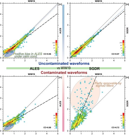
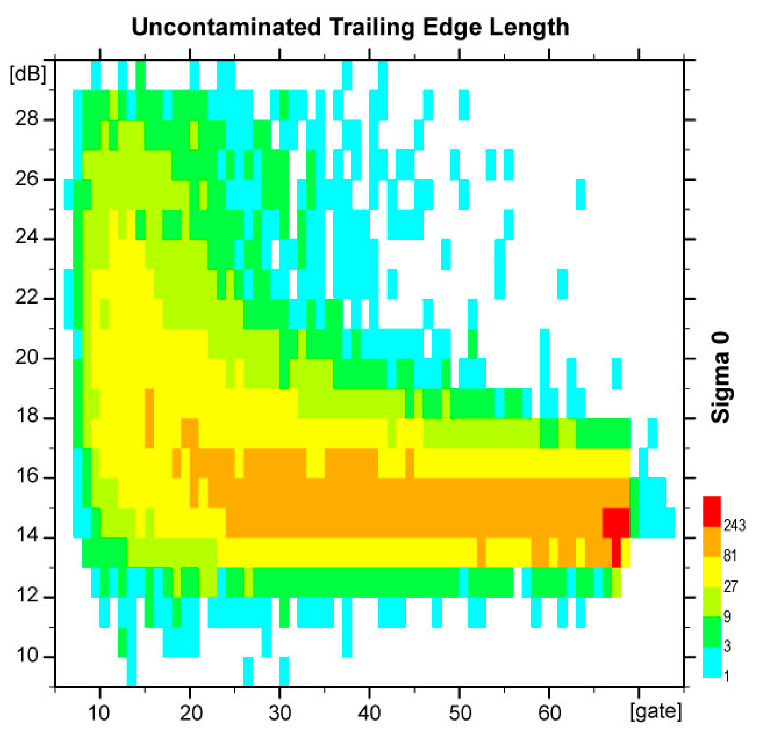
In the Celebes Sea where waveforms of satellite altimeters are often contaminated, two subwaveform retrackers, ALES and WIW19, are applied to Jason-2 20 Hz SGDR data. The estimated SWH datasets are first compared with the original SGDR SWH data that use full-length waveforms. Using radargrams, or a series of adjacent waveforms along Jason-2 tracks, WIW19 can provide an optimal index (the uncontaminated trailing edge length) how Jason-2 observation points are close to contamination sources such as slicks and lands.

When observations are close to these contamination sources, SGDR tends to estimate unrealistic SWH values with respect to two subwaveform retrackers, since contaminated echoes near the leading edge ruin the full-waveform SGDR retracker. Meanwhile, the subwaveform retrackers avoid to use contaminated echoes within the trailing edge of the waveforms, so that their SWH estimations are not affected by the presence of contamination sources. These contaminated observations could be filtered by sigma0 criteria since they tend to have larger sigma0 values as “sigma0 blooms”. Strict sigma0 filtering certainly reduces SWH outliers and improves data quality, but unnecessarily removes uncontaminated observations at the same time.

When uncontaminated full-length waveforms are available, all algorithms are well correlated, except that ALES retracker has a positive bias in a calm sea state (SWH < 1 m), whose state is not unusual in the calm semi-enclosed Celebes Sea. Due to this positive bias, ALES data include no SWH estimations smaller than 0.4 m, which is rather unrealistic in this calm study area. Under the calm sea state condition, ALES limits the subwaveform estimation window size to less than six gates, even though a longer window size were actually available since observations are uncontaminated. In other words, although a short estimation window size of ALES subwaveform retracker is useful to avoid potential contaminations in the trailing edge slope, it could be too short in the calm sea state to properly fit the Brown model to a waveform with the steep leading edge. Meanwhile, WIW19 retracker extends the size of the uncontaminated estimation windows as long as possible.

For moderate sea states (SWH > 1.5 m), agreement of two subwaveform retrackers using the Nelder-Mead fitting method (WIW19 and ALES) are excellent despite that the subwaveform estimation window sizes are significantly different. On the other hand, WIW19 tends to estimate slightly larger SWH values than SGDR that uses MLE4 fitting, although both use the similar estimation window sizes. Therefore, for uncontaminated altimeter observations in moderate sea states, choices of the fitting algorithms would influence the similarity of the results more significantly than the estimation window sizes.

These datasets are then compared with WW3 model results, resulting in good agreement especially when comparisons are limited to uncontaminated Jason-2 observations. Note, however, that WIW19 retracker can achieve similar agreement with all available observations without such strict limitation, providing better data availability; data availability would be especially important e.g., in assimilating fast-varying SWH field in coastal areas.

The agreement, however, becomes worse if swells from the Pacific is excluded in the WW3 model, suggesting that the swells are almost always present in the Celebes Sea, in spite of its semi-enclosed nature. Comparisons with individual Jason-2 data also reveal discrepancies that may be caused by insufficiency of the present WW3 model calculated from the NECEP wind fields, such as displacements of locally-confined SWH events with respect to Jason-2 tracks. Together with improved quality of the altimetry SWH data, higher resolutions of both wave models and wind fields would further improve wave fields descriptions in semi-enclosed coastal seas.

References

1. Zieger, S.; Vinoth, J.; Young, I.R. Join Calibration of Multiplatform Altimeter Measurements of Wind Speed and Wave Height over the Past 20 Years. J. Atmos. Ocean. Tech. 2009, 26, 2549–2564. [Google Scholar] [CrossRef]
2. Ribal, A.; Young, I.R. 33 years of globally calibrated wave height and wind speed data based on altimeter observations. Sci. Data 2019, 6, 1–15. [Google Scholar] [CrossRef] [Green Version]
3. Gommenginger, C.; Thibaut, P.; Fenoglio-Marc, L.; Quartly, G.; Deng, X.; Gomez-Enri, J.; Challenor, P.; Gao, Y. Retracking Altimeter Waveforms Near the Coasts. In Coastal Altimetry; Vignudelli, S., Kostianoy, A., Cipollini, P., Beneveniste, J., Eds.; Springer: Berlin/Heidelberg, Germany, 2011; pp. 61–102. [Google Scholar]
4. Wang, X.F.; Ichikawa, K. Coastal Waveform Retracking for Jason-2 Altimeter Data based on along-track Echograms around the Tsushima Islands in Japan. Remote Sens. 2017, 9, 762. [Google Scholar] [CrossRef] [Green Version]
5. Passaro, M.; Cipollini, P.; Vignudeli, S.; Quartly, G.D.; Snaith, H.M. ALES: A multi-mission adaptive subwaveform retracker for coastal and open ocean altimetry. Remote Sens. Environ. 2014, 145, 173–189. [Google Scholar] [CrossRef] [Green Version]
6. Wang, X.F.; Ichikawa, K.; Wei, D.G. Coastal waveform retracking in the slick-rich Sulawesi Sea of Indonesia, based on variable footprint size with homogeneous sea surface roughness. Remote Sens. 2019, 11, 1274. [Google Scholar] [CrossRef] [Green Version]
7. Idris, N.H.; Deng, X.; Md Din, A.H.; Idris, N.H. CAWRES: A Waveform Retracking Fuzzy Expert System for Optimizing Coastal Sea Levels from Jason-1 and Jason-2 Satellite Altimetry Data. Rem. Sens. 2017, 9, 603. [Google Scholar] [CrossRef] [Green Version]
8. Thibaut, P.; Poisson, J.C.; Bronner, E.; Picot, N. Relative Performance of the MLE3 and MLE4 Retracing Algorithms on Jason-2 Altimeter Waveforms. Mar. Geod. 2010, 33, 217–335. [Google Scholar] [CrossRef]
9. Dumont, J.P.; Rosmorduc, V.; Carrere, L.; Picot, N.; Bronner, E.; Couhert, A.; Desai, S.; Bonekamp, H.; Scharroo, R.; Leuliette, E. OSTM/Jason-2 Products Handbook, Iss. 1rev11, SALP-MU-M-OP-15815-CN; CNESS: Paris, France, 2017; pp. 1–66. [Google Scholar]
10. Passaro, M.; Fenoglio-Marc, L.; Cipollini, P. Validation of significant wave height from improved satellite altimetry in the German bight. IEEE Trans. Geosc. Rem. Sens. 2015, 53, 2146–2156. [Google Scholar] [CrossRef]
11. Tolman, H.L. User Manual and System Documentation of WAVEWATCH III TM Version 3.14; National Centers for Environmental Prediction, National Weather Service, NOAA: Camp Springs, MD, USA, 2009. [Google Scholar]
12. Saha, S.; Moorthi, S.; Wu, X.; Wang, J.; Nadiga, S.; Tripp, P.; Behringer, D.; Hou, Y.-T.; Chuang, H.-Y.; Iredell, M.; et al. The NCEP Climate Forecast System Version 2. J. Clim. 2014, 27, 2185–2208. [Google Scholar] [CrossRef]
13. Bidlot, J.R.; Janssen, P.A.E.M.; Adballa, S. A Revised Formulation of Ocean Wave Dissipation and Its Model Impact. ECMWF Technical Memoranda 509; ECMWF: Reading, UK, 2007; pp. 1–27. [Google Scholar] [CrossRef]
14. Hasselmann, S.; Hasselmann, K.; Allender, J.H.; Barnet, T.P. Computations and Parameterizations of the Nonlinear Energy Transfer in a Gravity-Wave Spectrum. Part II: Parameterizations of Nonlinear Energy Transfer for Application in Wave Models. J. Phys. Oceanogr. 1985, 15, 1378–1391. [Google Scholar] [CrossRef] [Green Version]
15. Chawla, A.; Spindler, D.M.; Tolman, H.L. Validation of a thirty year wave hindcast using the Climate Forecast System Reanalysis winds. Ocean Model. 2013, 70, 189–206. [Google Scholar] [CrossRef]
16. Perez, J.; Menendez, M.; Losada, I.J. GOW2: A global wave hindcast for coastal applications. Coast. Engin. 2017, 124, 1–11. [Google Scholar] [CrossRef]
17. Ribal, A.; Babanin, A.V.; Zieger, S.; Liu, Q.X. A high-resolution wave energy resource assessment of Indonesia. Renew. Energy 2020. [Google Scholar] [CrossRef]
18. Cavaleri, L.; Abdalla, S.; Benetazzo, A.; Bertotti, L.; Bidlot, J.-R.; Breivik, Ø.; Carniel, S.; Jensen, R.E.; Portilla-Yandun, J.; Rogers, W.E.; et al. Wave modelling in coastal and inner seas. Prog. Oceanogr. 2018, 167, 164–233. [Google Scholar] [CrossRef]
19. Wang, X.F.; Ichikawa, K. Effect of High-Frequency Sea Waves on Wave Period Retrieval from Radar Altimeter and Buoy Data. Remote Sens. 2016, 8, 764. [Google Scholar] [CrossRef] [Green Version]
20. Schlembach, F.; Passaro, M.; Quartly, G.D.; Kurekin, A.; Nencioli, F.; Dodet, G.; Piolle, J.F.; Ardhuin, F.; Bidlot, J.; Schwatke, C.; et al. Round Robin Assessment of Radar Altimeter Low Resolution Mode and Delay-Doppler Retracking Algorithms for Significant Wave Height. Rem. Sens. 2020, 12, 1254. [Google Scholar] [CrossRef] [Green Version]
Figure 1. Schematic waveform (a) and radargram (b) affected by an area of smooth sea surface. Waveforms of all latitudes in (b) are aligned with respect to the gate of the leading edge bottom. At a latitude y1 indicated by a red line in (b), the waveform behaves as in (a). Presence of a smooth surface area is recognized in (b) as an area of extraordinary-strong power of echoes shown with orange and yellow colors around a latitude y0, and which contaminates waveforms of neighboring latitudes as stronger echoes (with green color) from inhomogeneous reflectance within a footprint that do not follow the Brown model. The black and white lines in b indicate the stop gate of the subwaveform estimation window in WIW19 and Adaptive Leading Edge Subwaveform (ALES), respectively [6]. A green curve in (a) indicates the Brown mathematical model in WIW19 fitted excluding the contaminated trailing edge.
Remotesensing 12 03367 g001
Figure 2. Location of the Indonesian Seas, or the inner nest domain for the nested WAVEWATCH III version 3.14 (WW3) model. The Celebes Sea, or the study area of Jason-2 altimeter data, is highlighted as the green inner box. Four Jason-2 tracks are present in the Celebes Sea; tracks are indicated by red lines in the inner box with track numbers.
Remotesensing 12 03367 g002
Figure 3. Estimated significant wave height (SWH) values by WIW19 (green), ALES (red), and SGDR (blue) algorithms and WW3 model value (orange) along Track 190 in a standard calm sea state (21 May 2014 07:34) (a), or in a rougher sea state (12 January 2014 09:54) (b). The 18-km averaged values and their standard deviations are also indicated by lines.
Remotesensing 12 03367 g003
Figure 4. Histograms of Jason-2 20 Hz SWH data determined by WIW19 (a), ALES (b), and SGDR (c). Bin sizes are 0.1 m and the total data number is shown in each panel.
Remotesensing 12 03367 g004
Figure 5. Histograms of Jason-2 20 Hz SWH data determined by WIW19 (a), ALES (b), and SGDR (c). The same as Figure 4, but for 18-km averaged values.
Remotesensing 12 03367 g005
Figure 6. Scatter density plots of Jason-2 SWH values between WIW19 and ALES datasets (a), WIW19 and SGDR datasets (b), and ALES and SGDR datasets (c). Orthogonal regression lines are indicated by bold broken lines. Reference equivalence lines are also indicated by thin lines.
Remotesensing 12 03367 g006
Figure 7. Histograms of Jason-2 SWH data determined by WIW19 (a), ALES (b), and SGDR (c) and corresponding SWH values in WW3 wave model (d). Bin sizes are 0.1 m and the total data number is shown in each panel.
Remotesensing 12 03367 g007
Figure 8. All panels (ac) are the same as Figure 6, but between SWH in WW3 model and Jason-2 data determined by WIW19 (a), ALES (b), and SGDR (c).
Remotesensing 12 03367 g008
Figure 9. All panels (ac) are the same as Figure 6 but for observations near contamination sources (waveforms with the uncontaminated trailing edge (UTE) lengths less than 15 gates).
Remotesensing 12 03367 g009
Figure 10. All panels (ac) are the same as Figure 6 but for uncontaminated observations (waveforms with the UTE lengths larger than 60 gates). Additionally, orthogonal regression lines are calculated for two sections where the abscissa SWH is larger or smaller than 1.5 m and plotted by blue dotted lines.
Remotesensing 12 03367 g010
Figure 11. Scatter density plot between the UTE lengths and sigma0 values of 18-km averaged SGDR data.
Remotesensing 12 03367 g011
Figure 12. The same as Figure 6b but data are excluded when SGDR sigam0 is larger than 22 dB (a), 19 dB (b), 16 dB (c), and 15 dB (d).
Remotesensing 12 03367 g012
Figure 13. All panels (ac) are the same as Figure 8 but for uncontaminated observations (UTE length is larger than 60 gates).
Remotesensing 12 03367 g013
Figure 14. The same as Figure 13 but between non-nested WW3 model SWH and Jason-2 SWH from uncontaminated observations determined by WIW19 (a), ALES (b), and SGDR (c). Scatter density plot between non-nested WW3 model and WW3 model is also shown for reference (d). The reference equivalence lines for 0.6-m swell are plotted by red dotted lines.
Remotesensing 12 03367 g014
Figure 15. Scatter plots between WW3 and non-nested WW3 model results extracted at the Jason-2 uncontaminated observations. All values along Track 101 are indicated by circles, Track 012 by triangles, Track 025 by squares, and Track 190 by rhombuses. These marks are colored in red for observation points between 1 and 2°N, orange between 2 and 3°N, green between 3 and 4°N, cyan between 4 and 5°N, and blue between 5 and 6°N. Three lines plotted are the same as Figure 14d.
Remotesensing 12 03367 g015
Figure 16. The SWH field in the nested WW3 model (a) and the NCEP wind field (b) at 10:00 on 2014/01/12. Jason-2 passed along Track 190 (shown by purple broken lines) six minutes before, as shown in Figure 3b. Wind vectors in (b) are sparsely plotted with 0.5° gaps, and colored in blue, green and red when wind speed is less than 5 ms−1, from 5 to 10 ms−1, and more than 10 ms−1, respectively.
Remotesensing 12 03367 g016