Abstract
Anomaly detection is one of the most challenging topics in hyperspectral imaging due to the high spectral resolution of the images and the lack of spatial and spectral information about the anomaly. In this paper, a novel hyperspectral anomaly detection method called morphological profile and attribute filter (MPAF) algorithm is proposed. Aiming to increase the detection accuracy and reduce computing time, it consists of three steps. First, select a band containing rich information for anomaly detection using a novel band selection algorithm based on entropy and histogram counts. Second, remove the background of the selected band with morphological profile. Third, filter the false anomalous pixels with attribute filter. A novel algorithm is also proposed in this paper to define the maximum area of anomalous objects. Experiments were run on real hyperspectral datasets to evaluate the performance, and analysis was also conducted to verify the contribution of each step of MPAF. The results show that the performance of MPAF yields competitive results in terms of average area under the curve (AUC) for receiver operating characteristic (ROC), precision-recall, and computing time, i.e., 0.9916, 0.7055, and 0.25 s, respectively. Compared with four other anomaly detection algorithms, MPAF yielded the highest average AUC for ROC and precision-recall in eight out of thirteen and nine out of thirteen datasets, respectively. Further analysis also proved that each step of MPAF has its effectiveness in the detection performance.
1. Introduction
A hyperspectral image (HSI) is an image cube that consists of hundreds of spatial images of a particular space with different spectral information. It has better spectral information than a multispectral image because of its large number of narrow spectral bands [1]. Its rich information opens the possibility to differentiate several objects of interest based on their spectral signatures. Therefore, it is widely used in many remote-sensing research fields, such as spectral unmixing [2,3,4], target detection [5,6,7], and classification [8,9,10].
Target detection methods in HSI are mainly classified into supervised and unsupervised categories, based on the utilization of prior information. Anomaly detection is an unsupervised target detection method that aims to identify interesting objects that are different from their surroundings, in terms of spatial and spectral domain, without any prior information about the objects [11,12,13]. These objects consist of a relatively small number of pixels compared to the total number of pixels in the scene. Anomaly detection is widely used in many applications, such as urban detection [14], agriculture [15], maritime target detection, fire monitoring, and geology [16]. Hyperspectral anomaly detection has played a crucial role in both military [13,16,17] and civilian projects [13,14,18,19].
One of the important milestones in anomaly detection, developed by Reed and Yu, is the Reed–Xiaoli (RX) method [20]. It uses the multivariate Gaussian distribution to model the background. It then uses the Mahalanobis distance between the test pixel and the background to detect the anomaly. This method became well-known because of its simplicity and satisfying performance. Several extensions based on the RX were also proposed [21,22,23]. Recent algorithms based on RX and Fractional Fourier Entropy RX (FrFE-RX) [24] used the fractional Fourier transform as a preprocess to remove noise and to enhance the difference between the anomaly and the background. Even though this had a better performance than RX, it required a high computational time to do the preprocessing.
Another well-known approach in anomaly detection is collaborative-representation-based detector (CRD) [25]. This approach assumes that each pixel in the HSI can be approximately represented by its neighborhoods. The neighborhoods are defined by the area between the outer and the inner windows (dual windows) centered at each test pixel. This method, however, is not flexible. The performance of this method depends on the size of the dual windows. There is also a possibility that the anomalous pixels are inside the neighborhoods, which will decrease the performance of CRD. In order to address this issue, variants of CRD were proposed [26,27,28]. A recent algorithm, called spatial density background purification (SDBP) [29], also aimed to solve this problem. It used a density peak (DP) clustering algorithm to calculate the local density of the neighborhoods and remove some of the neighborhoods that have a low density to acquire pure background pixels in the neighborhoods. Even though the performance of the SDBP was better than that of CRD, this also depended on the size of dual windows. Another problem of CRD and its variants was the long computing time in detecting the anomalous pixels.
Another type of anomaly detection is based on the attribute filter that exploits HSI’s spatial information [30,31,32,33]. One of these methods, introduced by Kang et al., was called attribute and edge-preserving filters detector (AED) [33]. This assumed that anomalous pixels usually appear as small objects. AED used a principal component to reduce the HSI’s spectral resolution, the attribute filter to extract the anomalous pixels, and the edge-preserving filter for postprocessing to smooth the output detection and decrease the false alarm rate. This method had a good performance and fast computing time; however, the proposed filtering function introduced in [33] had a risk. This function was a filter that would remove an object if its area is greater than the filter threshold. If the location of anomalous objects was very close, the dilation process would combine those objects into one object. If the area of the combined object was greater than the filter threshold, this function would remove it. This would cause a significant decrease in AED’s performance. The other limitation of using AED was that the maximum area of the anomaly parameter needs to be set manually. Since AED used the attribute filter to extract the anomalous pixels and the area of the anomaly can differ in each HSI, this parameter was considered a crucial one due to its influence on the risk of false-positive and false-negative occurrences. Since the attribute filter was used to filter connected pixels based on the size area, false positive may occur if the size area is too wide so that there is one or more background pixels included in the anomalies. On the contrary, if the size area was too small, one or more anomaly pixels were excluded from the anomalies and considered as the background.
In this paper, we propose an algorithm for anomaly detection called morphological profile and attribute filter (MPAF). Different from previous works, our proposed method used a morphological profile [34] and an attribute filter [35] to detect anomalies in HSI. This study aims to improve the detection accuracy and computing time. This method is proposed based on the facts: (1) only some bands can give clear information about a certain object in HSI and some bands have a high correlation, and (2) anomalous objects are smaller than the background. Based on the first fact, entropy and histogram counts were used to select a band. This step was not only to select the effective band for anomaly detection but also to reduce the computing time of the algorithm. For the second fact, a morphological profile was used to extract the anomalous pixels and an attribute filter was used to filter the false anomalous pixels. Even though we can use an attribute filter to extract the anomalous pixels, it relies on the gray-level thresholds to label pixels in the image before extracting the anomalous pixels. The more complex the image is, the more ineffective it becomes. Meanwhile, the morphological profile extracted anomalous pixels in the image based on their neighborhood, but it was ineffective for removing large objects. Combining the morphological profile and the attribute filter for anomaly detection will improve the detection accuracy because they complement each other. Moreover, in order to address the issue of previous methods also based on the attribute filter, we propose an algorithm to automatically determine the maximum area of the anomaly.
Instead of using spectral signatures from all bands, several anomaly detection methods ([30,36,37,38]) applied band selection algorithm to reduce the spectral dimension, remove redundant and interference bands, and as a result, decrease false alarm rate. The selected bands had more discriminative features for anomaly than the discarded bands. This selection gave a positive effect on the performance of the subsequent detection algorithm and reduced the computational complexity. In this work, instead of spectral signatures, we used HSI data’s entropy as a means to observe the information quantity of the HSI bands. Entropy is a quantitative metric of the information contained in an image. This gave us a subset of prospective bands to represent the anomalies using a particular threshold. Since anomalies were much smaller than the background, we further selected one band from this subset using an algorithm based on the histogram that ensured the spatial characteristic between anomalies and the background. In addition, the subsequent step dealt with the algorithm to determine the maximum area of anomalies due to this spatial characteristic. Hence, even if there was a false anomalous pixel due to its same signature as the anomaly’s in the selected band, this algorithm can detect and remove it based on this spatial requirement. This paper shows that our proposed approach yielded superior results on thirteen datasets that are often used as a benchmark in HSI anomaly detection.
The contribution of this work is developing a new approach for HSI anomaly detection that combines two conventional techniques in image processing, added with new algorithms for band selection and determining the maximum area of anomalies. In the first step, the band selection contributes to less computing time while preserving the most representative band based on the entropy and histogram. Even though we applied conventional techniques for the next steps, we found that the results could be improved by suppressing the false-positive cases. Hence, in the filtering step, we propose the algorithm to determine the maximum area of anomalies automatically, that differs from previous works [30,31,32,33] in terms of automated fashion. This paper shows that the proposed algorithm increased detection performance by avoiding false-positive results.
The rest of this paper is organized as follows. Section 2 reviews the morphological profile and attribute filter. Section 3 describes the detail of the proposed method in this paper. Section 4 shows the parameter settings, results, and our respective analyses. Finally, Section 5 is the conclusion of this study.
2. Materials and Methods
2.1. Morphological Profile
A morphological profile consists of an opening profile and a closing profile [39], which are created based on mathematical morphology. A mathematical morphology [40] is a set of operations that processes objects in an image based on their shapes. Each pixel in the image is processed based on the value of other pixels in its neighborhood. The neighborhood is defined by the shape and size of the structuring element . There are two basic operations in mathematical morphology, i.e., erosion and dilation.
Erosion (⊖) is defined as a local minimum operator. It selects the minimum value between the manipulated pixel and its neighborhood. On the contrary, dilation (⊕) is defined as a local maximum operator. It selects the maximum value between the manipulated pixel and its neighborhood:
where is the domain of and is a grayscale image with indexes of spatial dimensions x and y. Erosion tends to remove bright pixels while dilation tends to remove dark pixels.
Other operations of mathematical morphology are called opening and closing, which are derived from erosion and dilation. Opening () and closing () are defined as follows:
Opening tends to remove bright pixels but is less destructive than erosion. Meanwhile, closing tends to remove dark pixels but is less destructive than dilation.
2.2. Attribute Filter
An attribute filter is an adaptive filter introduced by Breen and Jones [41]. It can preserve or remove connected components in an image based on a predefined attribute such as area, standard deviation, the moment of inertia, etc. Here, we briefly describe how the attribute filter worked. Refer to [35] for a detailed explanation.
Binary attribute thinning is defined as a filter that removes connected components of true pixels, called a binary connected opening, that does not fulfill criterion . For example, if given is the area that contains more than 25 pixels, preserves only the connected components that have more than 25 pixels and removes the others. Whereas, binary attribute thickening is defined as a filter that removes connected components of false pixels, called binary connected closing, that does not fulfill criterion .
A grayscale image can be represented as a stack of binary images obtained by thresholding the grayscale image at each of its gray levels. The connected components of a grayscale image are built based on this set of gray levels. If given a set of gray levels , ranging on the gray levels of , grayscale attribute thinning and thickening can be defined as follows:
where is the binary image obtained by thresholding at gray level . In other words, grayscale attribute thinning removes connected components of bright pixels that do not fulfill the criterion and grayscale attribute thickening removes connected components of dark pixels that do not fulfill the criterion .
2.3. Proposed Algorithm
Figure 1 shows that the proposed method, i.e., morphological profile and attribute filter (MPAF), consisted of three steps: (1) selecting a band based on entropy and histogram counts; (2) background removal with the morphological profile (MP); and (3) filtering the image with the attribute filter (AF).
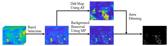
Figure 1.
Schematic of morphological profile and attribute filter (MPAF) algorithm for hyperspectral anomaly detection. MP—morphological profile, AF—attribute filter.
2.3.1. Entropy- and Histogram-Based Band Selection
There were three purposes of this band selection. The first was to classify the selected band as a bright-anomaly (BA) or dark-anomaly (DA) band. Bright-anomaly means the anomaly is shown as bright pixels in the image. Dark-anomaly means the anomaly is shown as dark pixels in the image. The second was to select the most effective band for anomaly detection. The third aimed to reduce computing time.
The adjacent bands of the HSI are highly correlated [30]. Processing all the bands will be inefficient. Therefore, the first step of the proposed band selection was sampling the band in the HSI as follows:
where is the index of the band to sample, is the sampling interval, is the starting band of the sample image, and is the sample image. Reducing the spectral resolution will reduce the computational cost.
The second step was classifying each sample image as and filtering them based on the most frequent classification. In this step, each sample image was normalized as follows:
where is pixel i of , is the normalized image, is the mean of pixels in the image , and is the standard deviation of pixels on the image .
The normalized image made a clear differentiation between background pixels and anomalous pixels. Figure 2 shows the differentiation between the data before and after normalization. Anomalous pixels are shown as small objects in the image, and the other pixels are background pixels, either in images before or after normalization. The histograms after normalization, however, are shifted and expanded so that it is more reliable to take a threshold to define whether the images belong to the band with BA (Figure 2a,b) or DA (Figure 2c,d). Let denote the threshold to define extreme-bright pixels (whose values v), and extreme-dark pixels (whose value ). Then, each sample image was then classified as follows:
where is the bright-anomaly band flag, is the dark-anomaly band flag, is the classification threshold, and is the normalized histogram counts at pixel value v.
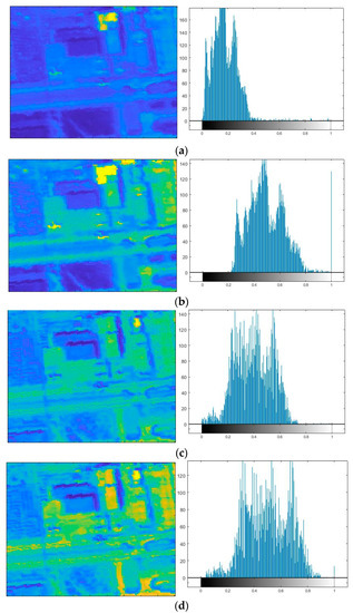
Figure 2.
Image and image histogram of (a) ABU-Airport-1 band 5 before normalization and (b) after normalization; and (c) band 165 before normalization and (d) after normalization. The histograms show the grayscale values (in the range of 0–1) in the -axis, and the number of pixels (counts) in the -axis.
The sample images were then filtered as follows:
where is a matrix that contains filtered images, and . is a matrix that contains bright-anomaly images, and is a matrix that contains dark-anomaly images.
In order to avoid using bands that contain noise, the samples were filtered using entropy (). Entropy was used to measure the information contained in the image. The filtered images () were calculated as follows:
where is the normalized histogram counts and is the element of . is the mean of entropy of all bands in I, and is the standard deviation of entropy of all bands in I. Figure 3 shows that bands with very low entropy, i.e., bands 148, 156, and 204, cannot be used for anomaly detection. Meanwhile, the other band with average entropy, i.e., band 6, can be used for anomaly detection.
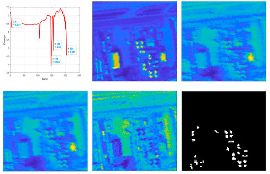
Figure 3.
(a) Entropy curve of all bands. Image of band (b) 6, (c) 148, (d) 156, and (e) 204. (f) Reference map.
The band was then selected as follows:
where is the selected band and is a selection coefficient. The image with the above condition will have more background pixels. Thus, this condition will improve the detection rate when using a morphological profile to detect anomalies.
2.3.2. Background Removal
Anomalies are shown as small dark or bright objects in the image. MP was used to detect these objects. Anomalies can be detected by the following equations:
where is the resulting image and , which represents the width of the anomaly, and is the width of square s. Opening removes small objects from bright pixels and closing removes small objects from dark pixels. Therefore, Equation (16) results in anomalous objects.
2.3.3. Area Filtering
Even though we can detect objects with MP, the shape of s is fixed [39]. They are ineffective on non-compact shapes, especially on large objects. Therefore, AF was used to filter these objects:
where is the differential map, is the maximum area of anomalous objects, is the output of the filter, is element-wise multiplication, and is the width of square . The criteria used in both attribute filters ( and ) is , which means they will keep the connected components whose area is greater than . Therefore, the differential map obtained by Equation (17) will remove the objects whose area is greater than . Since is used for filtering, dilating it with se3 will expand each area on to avoid losing anomalous pixels during the AF process.
2.3.4. Area of Anomaly
In previous works [30,31,32,33], the limitation of using AF was that the methods need to set the manually. Therefore, in this paper, we proposed a novel method to automatically set not only the but also the .
Anomalous objects in an image usually appear as small objects and have a similar area. We can differentiate the anomalous objects from the background even though they have a similar spectral reflectance. Based on these assumptions, if given a set of areas of suspected anomalous objects, we can model this set as a normal distribution. Thus, we can calculate the maximum area of anomalous objects statistically. Furthermore, to optimize the detection using MP with square , the width of should be equal to the width of the smallest square containing the anomalous object. It is equivalent to the maximum value between the width and height of the smallest box containing the anomalous object (bounding box).
To extract the suspected anomalous objects from the image, we proposed using differential map like in Equation (17). In [33], the optimal value for the maximum area of anomalous objects was set to be pixels, where is the number of pixels in HSI. Based on this, was first calculated with equal to . The Boolean map was then obtained by thresholding the as follows:
where is the threshold of the image. The value of is set with Otsu’s method [42] due to its robust performance. The connected components in represent the suspected anomalous objects. Each connected component in can be labeled. Then, we can get the area of each connected component and the width and height of each connected component’s bounding box.
We let be the areas of connected components in and be a set of widths and heights of connected components’ bounding boxes. and are calculated as follows:
where , is the mean of , is the standard deviation of , and .
3. Experimental Results and Analysis
3.1. Data
In this paper, the proposed method was evaluated on real datasets that have been made available online [43], i.e., Airport–Beach–Urban (ABU) datasets. The data were manually extracted from images of the Airborne Visible/Infrared Imaging Spectrometer (AVIRIS), except for ABU-Beach-4, which was manually extracted from the image of the Reflective Optical System Imaging Spectrometer (ROSIS-03). Each dataset had a reference map that has been manually labeled. Table 1 describes some features of these images.

Table 1.
Features of the Airport–Beach–Urban (ABU) datasets.
3.2. Results
The performance of MPAF was evaluated with the most widely used metrics, area under the curve (AUC), and the receiver operating characteristic (ROC) [44]. To verify the performance of the proposed method, other methods, i.e., RX [20], FrFE-RX [24], AED [33], and SDBP-D [29] (SDBP with dual window) detectors, were used for comparison. These methods were either frequently cited in the literature or recent algorithms for HSI anomaly-detection applications.
To generate the results in Table 2, optimal parameters of FrFE-RX, AED, SDBP-D methods were selected for each image to get the best AUC. For FrFE-RX, the fractional-order () was selected by varying it from 0–1. Since the same datasets were used in AED, we set the maximum area of the anomaly () for each dataset as the same as the values recommended in [33]. The other parameters of AED were kept at AED’s default parameter setting, i.e., , , , and . Similarly, for SDBP-D, we used the values recommended in [29] to set the window size ( and ) and the percentage of the highest selected density value ().
Table 2.
Area under the curve (AUC) values of receiver operating characteristic (ROC) curves for the compared methods, i.e., morphological profile and attribute filter (MPAF), Reed–Xiaoli (RX), fractional fourier entropy RX (FrFE-RX), attribute and edge-preserving filters detector (AED), and spatial density background purification with dual window (SDBP-D) on the ABU datasets.
For the proposed method, a default parameter setting (, ,, , and ) was used for most of the datasets, which will be discussed in the next subsection. This setting could achieve acceptable performances for most of the datasets. If only a small number of bands or no band can represent all anomalous pixels in the reference map, the needed to be adjusted. Specifically, for the ABU-Airport-1 and the ABU-Beach-4 datasets, the was set as .
As shown in Table 2, the MPAF method achieved the best scores on 61.5% of the datasets (8 out of 13 datasets). The average AUCs of the MPAF method on each ABU dataset were 0.9816, 0.9971, and 0.9962, respectively, and the average of all datasets reached 0.9916. Even though the MPAF method ranked second on the ABU-Airport datasets, the difference was only 0.0076, which is very low. The proposed method also achieved the best score on 50% of the ABU-Airport datasets. The result of the proposed method was also stable, as the minimum AUC score was 0.9718 (ABU-Airport-1). The FrFE-RX method showed better performances than the RX method in most cases, which was consistent with the results reported in [24]. Despite those results, the FrFE-RX’s AUCs still could not match the MPAF’s AUCs in all cases. Both the AED and the SDBP-D method performed well, but still less effectively than the proposed method.
Figure 4, Figure 5 and Figure 6 show the results obtained by the compared methods for the three scenes. As shown in those figures, anomalous objects can be easily recognized on the MPAF and the AED detection maps visually. On the contrary, it is harder to recognize anomalous objects on the RX and the FrFE-RX detection maps. Most of the MPAF results had fewer false anomalous pixels compared to the AED or the other methods. This means that the attribute filter with the determination of anomaly area proposed in this method was effective for removing false anomalous pixels. Moreover, the MPAF method can detect all anomalous objects even though it cannot wholly detect all of the pixels in the objects.
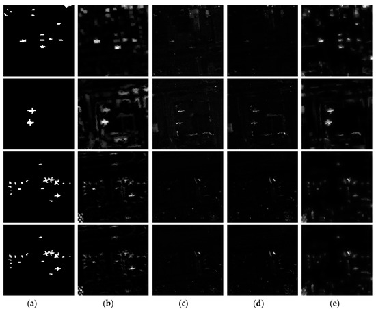
Figure 4.
ABU-Airport detection map of the compared methods. (a) Reference map, (b) MPAF, (c) RX, (d) FrFE-RX, (e) AED.
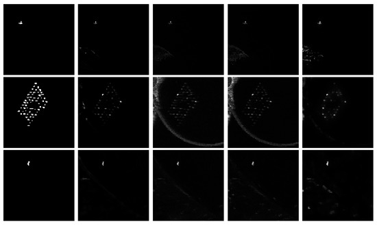
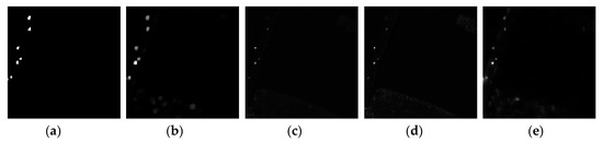
Figure 5.
ABU-Beach detection map of the compared methods. (a) Reference map, (b) MPAF, (c) RX, (d) FrFE-RX, (e) AED.
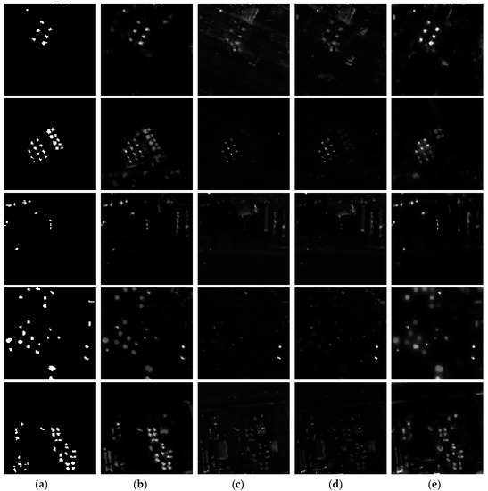
Figure 6.
ABU-Urban detection map of the compared methods. (a) Reference map, (b) MPAF, (c) RX, (d) FrFE-RX, (e) AED.
Although the performance of AED was relatively stable, its AUC score was very low, i.e., 0.789, on the ABU-Urban-2 dataset. It was the result of performing image dilation before performing its filtering function. As shown in Figure 6, the anomalous objects were very close to each other. Two or more anomalous objects merged into one after the image dilation step. As a result, the area of the merged objects was greater than the threshold of the filtering function. Meanwhile, our proposed algorithm avoided this drawback by the step to determine the area of anomaly.
Figure 7, Figure 8 and Figure 9 show the ROC curves of different methods, i.e., the MPAF, RX, FrFE-RX, and AED methods, for anomaly detection using the ABU datasets. The probability of the detection of MPAF is always greater than 0.9 before the false-alarm rate reaches 0.1. It means that for a low false-alarm rate, the result of the proposed method has promising results.
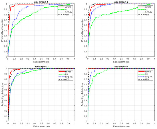
Figure 7.
ROC curves of the compared methods on the ABU-Airport Scene.
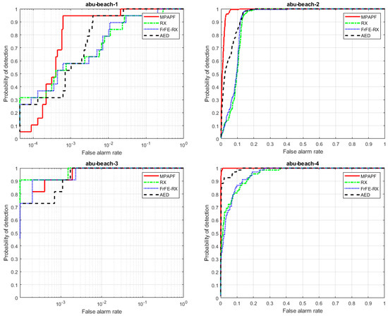
Figure 8.
ROC curves of the compared methods on the ABU-Beach Scene.
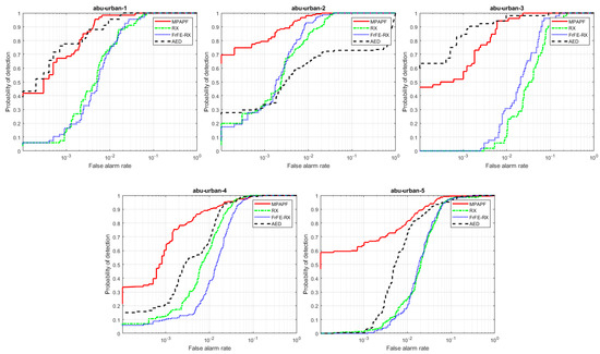
Figure 9.
ROC curves of the compared methods on the ABU-Urban Scene.
In observation, since imbalanced datasets may occur between anomaly and background classes, we also evaluated the performance using precision-recall curve. Instead of using the F1-score that summarizes a method’s performance for a specific probability threshold, a precision-recall curve provided the performance across different thresholds by its AUC. Figure 10, Figure 11 and Figure 12 depict the precision-recall curves of the compared methods for Airport, Beach, and Urban datasets, respectively. Table 3 shows the AUC values of each curve. One can see that MPAF outperformed the other methods in most cases, i.e., nine out of thirteen datasets with the average value reached 0.7055, which is 0.1080 higher than the second-best method, i.e., AED. Based on these results and the definition of precision and recall, it implies that MPAF was the best approach among others in predicting positive anomalies while reducing false ones and capturing the actual anomalies on the scenes.
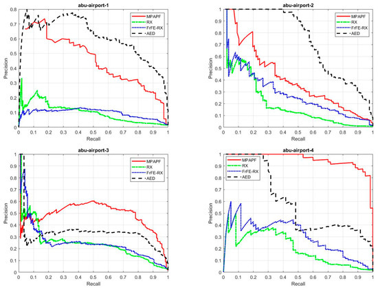
Figure 10.
Precision-recall curves of the compared methods on the ABU-Airport Scene.
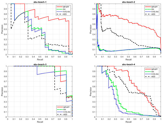
Figure 11.
Precision-recall curves of the compared methods on the ABU-Beach Scene.
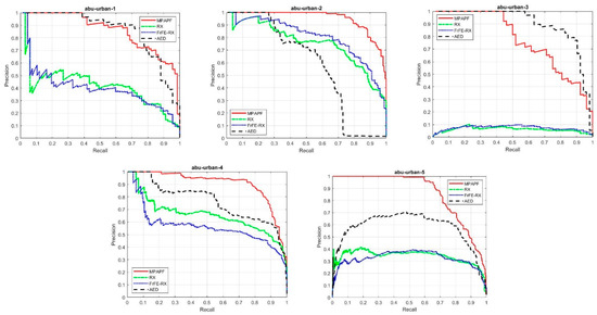
Figure 12.
Precision-recall curves of the compared methods on the ABU-Urban Scene.
Table 3.
AUC values of precision-recall curves for the compared methods on the ABU datasets.
4. Discussion
4.1. Computing Time
In this paper, the computing time of the MPAF is also compared with the other methods. All methods were executed using MATLAB on a computer with Intel(R) Core(TM) i5–4300U CPU and 16 GB RAM. The results are shown in Table 4. It was shown that the proposed method’s time is quite fast, ranking second after the RX method. The differences were not too significant (0.03–0.11 s). Moreover, even though the RX method was fast, the AUC results of this method were far less accurate than the AUC results of the proposed method. As expected from the FrFE-RX method, even though it is a modification of the RX method, it required a lot of time to process the datasets and to select the optimum fractional-order, since this process is pixel-based and is done for each band. The computing time of the proposed method should be acceptable since it had promising results.
Table 4.
The average computing time (in seconds) of the compared methods on the ABU dataset.
4.2. Component Analysis
This subsection analyzes the influence of different parameters on the performance of the MPAF method, the effectiveness of its band-selection method, and the effect of the MP and AF combination on the detection method. These parameters were the maximum area of the anomalous objects and the width-of-square s, i.e., , , and . AUC was used to evaluate the performance of the MPAF method under different parameter settings.
4.2.1. Parameter Sensitivity Analysis
Figure 13 shows the average AUCs of the MPAF on each dataset under the influence of different parameter settings. When analyzing the influence of one parameter, the other parameter was set with the default parameter settings , ,, , and . Both and were set automatically when analyzing and , since they did not depend on other parameters but images. Either or was set automatically when analyzing one of these parameters.
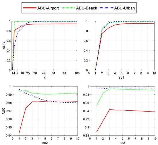
Figure 13.
Influence of the parameters, , , , and over the MPAF performance.
As shown at the top of Figure 13, the AUCs depended on the area of the anomaly in the MPAF method, i.e., and . The average of AUCs increased from zero before they saturated on a particular value. If either was less than the area of the anomaly or was less than the width of the anomaly, the accuracy of detection was low. It means that the proposed algorithm for setting and was proved to be effective since the AUCs in Table 2 were above 0.97. Furthermore, in a particular case, e.g., ABU-Urban-3, some objects had the same reflectance value as the anomaly. Therefore, if either was greater than the area of the anomaly or was greater than the width of the anomaly, some false anomalous pixels were detected and reduced the AUC of MPAF, as shown in Figure 14.
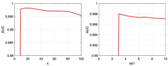
Figure 14.
Influence of parameters and over the MPAF performance on the ABU-Urban-3 dataset.
The bottom left of Figure 13 shows the influence of over the detection performance. In the ABU-Urban and ABU-Beach cases, increasing decreased detection performance. This meant that in most cases, the dilation step with was not needed, since means there was no dilation. In the ABU-Airport case, Figure 15a shows the influence of over AUCs for all the ABU-Airport datasets. It clearly shows that only ABU-Airport-1 needed the dilation step. Furthermore, at , Figure 15b shows that the maximum of AUCs was 0.8919. This means that the MPAF detected most of the anomaly locations, but not the entire area of each detected anomaly. After the dilation step, the detected anomalous objects were expanded, thus increasing the detection accuracy.
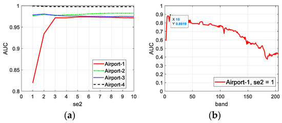
Figure 15.
(a) Influence of the parameter over the MPAF performance on the ABU-Airport datasets. (b) The MPAF performance on the ABU-Airport-1 dataset at .
The bottom right of Figure 13 shows the influence of over the detection performance. As expected, the AUCs increased when was increased to a certain value, i.e., . The dilation of the attribute filter expanded the objects in the image. Thus, the objects covered the lost pixels, which were caused by the AF process. The performance went down as was increased further, causing the objects to expand too much. Some false anomalous pixels were detected and reduced the AUC of MPAF.
4.2.2. Band Selection Effectiveness
To analyze the effectiveness of the proposed band selection, we compared the AUCs in Table 2 with the best AUCs of the MPAF without the band selection. The best AUCs were obtained by running the MPAF on each band of each dataset with the same parameter setting as the one that produced the AUCs in Table 2. Then we selected the maximum AUCs from each dataset. This comparison is shown in Table 5. The average differences of the AUC on the ABU datasets were 0.005125, 0.000615, and 0.0008, respectively. Even though the band selection process cannot obtain the best result, its performance is still acceptable since the differences were very low while promoting an automatic process. Furthermore, the time consumed was also low because of the spectral resolution reduction due to this band-selection process.
Table 5.
Comparison between AUC of the MPAF’s best band and AUC of the MPAF’s selected band on the ABU datasets.
4.2.3. MP and AP Effectiveness
To analyze the effect of MP and AF combination on the detection method, we compared the average AUCs of the MPAF in Table 2 with the average AUCs of the MPAF without MP and the MPAF without AF. As shown in Figure 16, the average AUCs of MPAF were always the highest, while the other two AUCs were inconsistent, depending on the datasets. In addition, we evaluated the statistics using a box plot, as shown in Figure 17. The first three boxes from the left correspond to Airport scenes that are performed by MPAF, MPAF without AF, and MPAF without MP, respectively. The following three boxes are for Beach, and the last three are for Urban scenes. One can see that compared with MP without AF and MP without AF, MPAF always showed the highest median values, least dispersed, and the highest minimum AUC values. It proved that combining MP and AF for anomaly detection improves the detection performance.
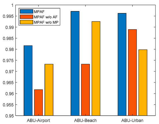
Figure 16.
Average AUCs of ROC for MPAF, MPAF without attribute filter (AF) step, and MPAF without morphological profile (MP) step on the ABU datasets.
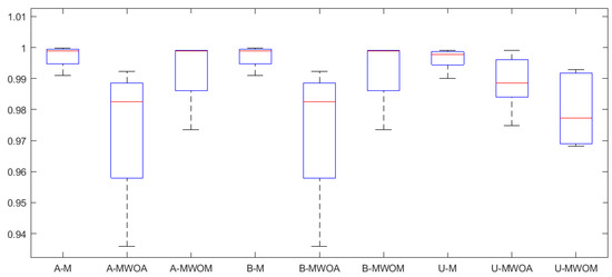
Figure 17.
Statistic of AUCs of ROC for different scenarios. From left to right, the first letter of the box’s name: A, B, U denotes the datasets, i.e., Airport, Beach, and Urban, respectively, followed by M, MWOA, or MWOM which are for the scenarios, i.e., MPAF, MPAF without AF, and MPAF without MP, respectively.
5. Conclusions
In this paper, we proposed a new hyperspectral anomaly detection algorithm called MPAF, based on the conventional morphological profile and attribute filter that improved with novel band selection and maximum area determination algorithms. This approach uses entropy and histogram counts to reduce the spectral dimension of the hyperspectral image, applies the morphological profile to discard the background pixels, and the attribute filter with a proposed area determination algorithm to filter the false anomalous pixels. A sensitivity analysis was conducted and proved the effectiveness of each step of the method. The experiments on real hyperspectral images showed that MPAF achieved high detection performances, reaching 0.9916 on average and superiority in 61.5% of thirteen datasets, with only slight differences in 38.5% of cases. In addition, it involved less computing time, i.e., 0.25 s on average. The performance of MPAF in reducing false anomalous pixels was also proven by reaching the highest score in the area under precision-recall curves, which was 0.1080 points higher than that of the state-of-the-art method. This proves that the proposed method is suitable for high-resolution HSIs and offers higher performance than previous methods.
Author Contributions
Conceptualization, F.A. and M.R.; methodology, F.A. and M.R.; software, F.A.; validation, M.R. and M.O.; formal analysis, F.A. and M.R.; data curation and writing—original draft preparation, F.A.; writing—review and editing, M.R. and M.O.; visualization, F.A.; supervision, M.R.; project administration, M.R.; funding acquisition, M.R. All authors have read and agreed to the published version of the manuscript.
Funding
This research was supported by Universitas Indonesia through Hibah Publikasi Artikel di Jurnal Internasional Kuartil Q1 dan Q2 (Q1Q2) research grant, under contract number NKB-0309/UN2.R3.1/HKP.05.00/2019.
Acknowledgments
The authors acknowledge the funding support.
Conflicts of Interest
The authors declare no conflict of interest.
References
- Rizkinia, M.; Okuda, M. Local abundance regularization for hyperspectral sparse unmixing. In Proceedings of the 2016 Asia-Pacific Signal and Information Processing Association Annual Summit and Conference (APSIPA), Jeju, Korea, 13–16 December 2016; pp. 1–6. [Google Scholar]
- Rizkinia, M.; Okuda, M. Joint Local Abundance Sparse Unmixing for Hyperspectral Images. Remote Sens. 2017, 9, 1224. [Google Scholar] [CrossRef]
- Kizel, F.; Benediktsson, J.A. Spatially Enhanced Spectral Unmixing through Data Fusion of Spectral and Visible Images from Different Sensors. Remote Sens. 2020, 12, 1255. [Google Scholar] [CrossRef]
- Zeng, Y.; Ritz, C.; Zhao, J.; Lan, J. Attention-Based Residual Network with Scattering Transform Features for Hyperspectral Unmixing with Limited Training Samples. Remote Sens. 2020, 12, 400. [Google Scholar] [CrossRef]
- Fu, X.; Shang, X.; Sun, X.; Yu, H.; Song, M.; Chang, C.-I. Underwater Hyperspectral Target Detection with Band Selection. Remote Sens. 2020, 12, 1056. [Google Scholar] [CrossRef]
- Moeini Rad, A.; Abkar, A.A.; Mojaradi, B. Supervised Distance-Based Feature Selection for Hyperspectral Target Detection. Remote Sens. 2019, 11, 2049. [Google Scholar] [CrossRef]
- Wu, X.; Zhang, X.; Wang, N.; Cen, Y. Joint Sparse and Low-Rank Multi-Task Learning with Extended Multi-Attribute Profile for Hyperspectral Target Detection. Remote Sens. 2019, 11, 150. [Google Scholar] [CrossRef]
- Fang, B.; Bai, Y.; Li, Y. Combining Spectral Unmixing and 3D/2D Dense Networks with Early-Exiting Strategy for Hyperspectral Image Classification. Remote Sens. 2020, 12, 779. [Google Scholar] [CrossRef]
- Liu, Y.; Gao, L.; Xiao, C.; Qu, Y.; Zheng, K.; Marinoni, A. Hyperspectral Image Classification Based on a Shuffled Group Convolutional Neural Network with Transfer Learning. Remote Sens. 2020, 12, 1780. [Google Scholar] [CrossRef]
- He, Z.; He, D. Spatial-Adaptive Siamese Residual Network for Multi-/Hyperspectral Classification. Remote Sens. 2020, 12, 1640. [Google Scholar] [CrossRef]
- Yang, Y.; Zhang, J.; Song, S.; Liu, D. Hyperspectral Anomaly Detection via Dictionary Construction-Based Low-Rank Representation and Adaptive Weighting. Remote Sens. 2019, 11, 192. [Google Scholar] [CrossRef]
- Tan, K.; Hou, Z.; Ma, D.; Chen, Y.; Du, Q. Anomaly Detection in Hyperspectral Imagery Based on Low-Rank Representation Incorporating a Spatial Constraint. Remote Sens. 2019, 11, 1578. [Google Scholar] [CrossRef]
- Ma, D.; Yuan, Y.; Wang, Q. Hyperspectral Anomaly Detection Based on Separability-Aware Sample Cascade. Remote Sens. 2019, 11, 2537. [Google Scholar] [CrossRef]
- Rodríguez-Cuenca, B.; García-Cortés, S.; Ordóñez, C.; Alonso, M.C. Automatic Detection and Classification of Pole-Like Objects in Urban Point Cloud Data Using an Anomaly Detection Algorithm. Remote Sens. 2015, 7, 12680–12703. [Google Scholar] [CrossRef]
- Horstrand, P.; Díaz, M.; Guerra, R.; López, S.; López, J.F. A Novel Hyperspectral Anomaly Detection Algorithm for Real-Time Applications with Push-Broom Sensors. IEEE J. Sel. Top. Appl. Earth Obs. Remote Sens. 2019, 12, 4787–4797. [Google Scholar] [CrossRef]
- Manolakis, D.; Truslow, E.; Pieper, M.; Cooley, T.; Brueggeman, M. Detection algorithms in hyperspectral imaging systems: An overview of practical algorithms. IEEE Signal Proc. Mag. 2014, 31, 24–33. [Google Scholar] [CrossRef]
- Chen, F.; Ren, R.; Van de Voorde, T.; Xu, W.; Zhou, G.; Zhou, Y. Fast Automatic Airport Detection in Remote Sensing Images Using Convolutional Neural Networks. Remote Sens. 2018, 10, 443. [Google Scholar] [CrossRef]
- Makki, I.; Younes, R.; Francis, C.; Bianchi, T.; Zucchetti, M. A Survey of Landmine Detection using Hyperspectral Imaging. ISPRS J. Photogramm. Remote Sens. 2017, 124, 40–53. [Google Scholar] [CrossRef]
- Taghipour, A.; Ghassemian, H. Hyperspectral Anomaly Detection Using Spectral–Spatial Features Based On the Human Visual System. Int. J. Remote Sens. 2019, 40, 8683–8704. [Google Scholar] [CrossRef]
- Reed, I.S.; Yu, X. Adaptive Multiple-Band CFAR Detection of an Optical Pattern with Unknown Spectral Distribution. IEEE Trans. Acoust. Speech Signal Process. 1990, 38, 1760–1770. [Google Scholar] [CrossRef]
- Zhou, J.; Kwan, C.; Ayhan, B.; Eismann, M.T. A Novel Cluster Kernel RX Algorithm for Anomaly and Change Detection Using Hyperspectral Images. IEEE Trans. Geosci. Remote Sens. 2016, 54, 6497–6504. [Google Scholar] [CrossRef]
- Imani, M. RX Anomaly Detector with Rectified Background. IEEE Geosci. Remote Sens. Lett. 2017, 14, 1313–1317. [Google Scholar] [CrossRef]
- Wang, W.; Zhao, B.; Feng, F.; Nan, J.; Li, C. Hierarchical Sub-Pixel Anomaly Detection Framework for Hyperspectral Imagery. Sensors 2018, 18, 3662. [Google Scholar] [CrossRef] [PubMed]
- Tao, R.; Zhao, X.; Li, W.; Li, H.; Du, Q. Hyperspectral Anomaly Detection by Fractional Fourier Entropy. IEEE J. Sel. Top. Appl. Earth Obs. Remote Sens. 2019, 12, 4920–4929. [Google Scholar] [CrossRef]
- Li, W.; Du, Q. Collaborative Representation for Hyperspectral Anomaly Detection. IEEE Trans. Geosci. Remote Sens. 2015, 53, 1463–1474. [Google Scholar] [CrossRef]
- Vafadar, M.; Ghassemian, H. Hyperspectral Anomaly Detection Using Outlier Removal from Collaborative Representation. In Proceedings of the International Conference on Pattern Recognition and Image Analysis, Shahrekord, Iran, 19–20 April 2017; pp. 13–19. [Google Scholar]
- Su, H.; Wu, Z.; Du, Q.; Du, P. Hyperspectral Anomaly Detection Using Collaborative Representation With Outlier Removal. IEEE J. Sel. Top. Appl. Earth Obs. Remote Sens. 2018, 11, 5029–5038. [Google Scholar] [CrossRef]
- Tan, K.; Hou, Z.; Wu, F.; Du, Q.; Chen, Y. Anomaly Detection for Hyperspectral Imagery Based on the Regularized Subspace Method and Collaborative Representation. Remote Sens. 2019, 11, 1318. [Google Scholar] [CrossRef]
- Tu, B.; Li, N.; Liao, Z.; Ou, X.; Zhang, G. Hyperspectral Anomaly Detection via Spatial Density Background Purification. Remote Sens. 2019, 11, 2618. [Google Scholar] [CrossRef]
- Xie, W.; Jiang, T.; Li, Y.; Jia, X.; Lei, J. Structure Tensor and Guided Filtering-Based Algorithm for Hyperspectral Anomaly Detection. IEEE Trans. Geosci. Remote Sens. 2019, 57, 4218–4230. [Google Scholar] [CrossRef]
- Lei, J.; Xie, W.; Yang, J.; Li, Y.; Chang, C. Spectral–Spatial Feature Extraction for Hyperspectral Anomaly Detection. IEEE Trans. Geosci. Remote Sens. 2019, 57, 8131–8143. [Google Scholar] [CrossRef]
- Taghipour, A.; Ghassemian, H. Hyperspectral anomaly detection using attribute profiles. IEEE Geosci. Remote Sens. Lett. 2017, 14, 1136–1140. [Google Scholar] [CrossRef]
- Kang, X.; Zhang, X.; Li, S.; Li, K.; Li, J.; Benediktsson, J.A. Hyperspectral Anomaly Detection with Attribute and Edge-Preserving Filters. IEEE Trans. Geosci. Remote Sens. 2017, 55, 5600–5611. [Google Scholar] [CrossRef]
- Benediktsson, J.A.; Palmason, J.A.; Sveinsson, J.R. Classification of Hyperspectral Data from Urban Areas Based on Extended Morphological Profiles. IEEE Trans. Geosci. Remote Sens. 2005, 43, 480–491. [Google Scholar] [CrossRef]
- Mura, M.D.; Benediktsson, J.A.; Waske, B.; Bruzzone, L. Morphological Attribute Profiles for the Analysis of Very High Resolution Images. IEEE Trans. Geosci. Remote Sens. 2010, 48, 3747–3762. [Google Scholar] [CrossRef]
- Xie, W.; Li, Y.; Lei, J.; Yang, J.; Chang, C.; Li, Z. Hyperspectral Band Selection for Spectral–Spatial Anomaly Detection. IEEE Trans. Geosci. Remote Sens. 2020, 58, 3426–3436. [Google Scholar] [CrossRef]
- Wang, L.; Chang, C.I.; Lee, L.C.; Wang, Y.; Xue, B.; Song, M.; Yu, C.; Li, S. Band Subset Selection for Anomaly Detection in Hyperspectral Imagery. IEEE Trans. Geosci. Remote Sens. 2017, 55, 4887–4898. [Google Scholar] [CrossRef]
- Prasad, S.; Bruce, L.M. Limitations of Principal Components Analysis for Hyperspectral Target Recognition. IEEE Geosci. Remote Sens. Lett. 2008, 5, 625–629. [Google Scholar] [CrossRef]
- Ghamisi, P.; Mura, M.D.; Benediktsson, J.A. A Survey on Spectral–Spatial Classification Techniques Based on Attribute Profiles. IEEE Trans. Geosci. Remote Sens. 2015, 53, 2335–2353. [Google Scholar] [CrossRef]
- Haralick, R.M.; Sternberg, S.R.; Zhuang, X. Image Analysis Using Mathematical Morphology. IEEE Trans. Pattern Anal. Mach. Intell. 1987, PAMI-9, 532–550. [Google Scholar] [CrossRef]
- Breen, E.J.; Jones, R. Attribute Openings, Thinnings, and Granulometries. Comput. Vis. Image Underst. 1996, 64, 377–389. [Google Scholar] [CrossRef]
- Otsu, N. A Threshold Selection Method from Gray-Level Histograms. IEEE Trans. Syst. Man Cybern. 1979, 9, 62–66. [Google Scholar] [CrossRef]
- Airport–Beach–Urban (ABU) Dataset. Available online: http://xudongkang.weebly.com/data-sets.html (accessed on 23 November 2019).
- Ferri, C.; Hernández-Orallo, J.; Flach, P. A Coherent Interpretation of AUC as a Measure of Aggregated Classification Performance. In Proceedings of the 28th International Conference on Machine Learning (ICML-11), Washington, DC, USA, 28 June–2 July 2011; pp. 657–664. [Google Scholar]


Publisher’s Note: MDPI stays neutral with regard to jurisdictional claims in published maps and institutional affiliations. |
© 2020 by the authors. Licensee MDPI, Basel, Switzerland. This article is an open access article distributed under the terms and conditions of the Creative Commons Attribution (CC BY) license (http://creativecommons.org/licenses/by/4.0/).