Robust Statistical Detection of GNSS Multipath Using Inter-Frequency C/N₀ Differences

Abstract

Multipath detection and mitigation are crucial issues for global navigation satellite system (GNSS) high-precision positioning. The multi-frequency carrier power-to-noise density ratio (C/N₀)-based multipath detection technique has achieved good results in real-time static and low-dynamic applications, and shown better practicability because of the low computational load and the requirement for little additional hardware. However, the classic multipath detection method based on inter-frequency C/N₀ differences directly employs the 3σ rule to determine the threshold without considering the distribution of detection statistics and their variation characteristics with elevation angle, and ignores the interference of outliers to the reference functions. A robust multipath detection method is proposed in this paper. The reference functions of C/N₀ differences are fitted using least absolute deviation (LAD) to obtain more accurate nominal values. According to the skew characteristics of the detection statistics, a medcouple (MC)-based adjusted boxplot is employed to determine the threshold. The performance of the new detection method is verified in the multipath environments. The experimental results show that compared with the classic method, the new multipath detector has strong robustness and can respond more accurately to large changes in multipath (MP) combination values at most elevation angles. It is sensitive to short-delay multipath and diffraction, and is an important supplement to multipath detection techniques.

1. Introduction

Multipath is one of the most problematic factors that restricts the accuracy and reliability of global navigation satellite system (GNSS) positioning, especially in challenging environments, such as urban canyons, viaducts, high-rise glass buildings and wooded areas. Due to the complexity of its generation mechanism, it is difficult to establish a general and accurate error model. Additionally, multipath depends on the surrounding environment of the receiver, so it cannot be eliminated by the double-differenced technique. According to the delay relative to the line-of-sight (LOS) signal, multipath can be divided into short-delay, medium-delay and long-delay multipath. Short-delay multipath is defined as reflected signal delays less than 0.1 chips (about 30 m for the GPS L1 C/A case) and long-delay multipath covers the reflected signal delays greater than 0.75 chips [1]. The latter can be distinguished easily by the code tracking loop of a GPS receiver, while short-delay multipath is often difficult to handle due to the strong correlation between its signal and the LOS signal [2]. Over the years, researchers have conducted extensive and in-depth research on multipath detection and mitigation [3,4,5,6,7,8]. However, no single method is completely reliable and suitable for all application scenarios. Thanks to the advancement of major GNSS constellations around the world and the popularity of multi-frequency receivers using both high-cost (Leica, Trimble, TopCon, Javad, etc.) and low-cost chipsets (u-blox F9P, Broadcom BCM47755, etc.), it has become increasingly attractive to reduce multipath and non-line-of-sight (NLOS) errors by using multi-frequency measurements [9,10,11,12]. Among them, multi-frequency carrier power-to-noise density ratio (C/N₀)-based multipath detection shows great potential in real-time applications because it does not require additional hardware and the computational load is low [13,14].

Since the phase of the reflected signal relative to its direct signal is wavelength dependent, different frequencies will cause different disturbances to the LOS component of the signal, resulting in different phase variations and power losses [15]. Therefore, the C/N₀ difference between two frequencies becomes an ideal indicator for assessing multipath interference. According to a nonlinear relationship between antenna gain and elevation angle, Strode and Groves [16] established a polynomial model of GPS C/N₀ difference with respect to elevation angle in a low-multipath environment, namely the reference function, and determined whether multipath exists by calculating the deviation degree between C/N₀ difference and its corresponding nominal value in a potential high-multipath environment. This method is suitable for geodetic applications and shows good performance in the detection of short-delay multipath and diffraction based on three-frequency C/N₀ measurements. Subsequently, Zhang et al. [17] extended the idea to GPS dual-frequency receivers. Nevertheless, the classic method actually falls into a statistical trap. The multipath detection statistics from calibration data do not follow the normal distribution, so it is not robust to determine the threshold using the 3σ rule based on the mean value and standard deviation. Špánik et al. [18] noticed this and have reconstructed the detection statistics to be closer to the zero-mean normal distribution, and then employed the 3σ rule to obtain the multipath detection threshold. However, the additional independent variables make the model more complex and its physical meaning seems ambiguous. Moreover, it is difficult for these new statistics to approach the zero-mean normal distribution at some elevation angles in practical applications.

In outlier detection for univariate data, the 3σ rule is the most commonly used statistics-based method. It is believed that almost all sample values are within three standard deviations of the mean, so it is empirically useful to consider 99.7% probability as close to certainty, and values outside this range are identified as outliers. However, the premise is that the data must follow a normal distribution. The detection statistics in the classic method are not normally distributed data at a specific elevation angle, but non-negative skewed data, that is, outliers only appear on one side of the distribution. In addition, although mean and standard deviation can be sensitive to the variations of sample data, such high sensitivity makes the detection method easy to be influenced by extreme values and thus cause misjudgment. Therefore, the 3σ rule cannot be simply used to determine the multipath detection threshold. An alternative outlier detection method for univariate data is the boxplot, proposed by Tukey [19]. Observations beyond the fence (Q₁ − 1.5IQR, Q₃ + 1.5IQR) are considered outliers, where Q₁ and Q₃ are the first and third quartiles, respectively; IQR = Q₃ − Q₁ is the interquartile range. For normally distributed data, the proportion of observations outside the fence is only 0.7%, namely 0.35% on each side of the distribution. Due to the use of quantiles instead of mean and standard deviation, boxplot has better robustness and is widely used in various fields. However, the boxplot only applies to normal or symmetric distributions and may not perform well for asymmetrical or heavy-tailed distributions. In order to make the boxplot useful for outlier detection in skewed data, statisticians have made some improvements to it [20,21,22,23,24]. However, these methods either do not sufficiently adjust for skewness or are not robust enough for outliers. Hubert and Vandervieren [25] proposed a new adjusted boxplot based on a robust measure of skewness, which can be applied to all distributions and is independent of the sample size. By establishing functions of the measure to adjust fences, the method takes into full account the skewness of the data and is resistant to outliers.

Another issue that cannot be ignored is the influence of outliers on the coefficient estimation of reference functions. Even in low-multipath environments, calibration data still include a certain number of abnormal measurements. The least squares estimation is sensitive to outliers, which may bias the regression line to outliers and cause the nominal value of the C/N₀ difference to be distorted. Therefore, it is necessary to introduce a robust regression method in the modeling process of reference functions to ensure the high accuracy of the nominal value. The simplest way to estimate parameters in a regression model, which is less sensitive to outliers than the least squares estimation, is to use the least absolute deviation (LAD) method [26]. Besides, to determine the multipath detection threshold using the new adjusted boxplot method, the first and third quantile functions with respect to elevation angle need to be calculated through quantile regression [27,28] after the statistic is obtained. Note that the LAD estimation is a special case of quantile regression where the quantile is equal to 0.5.

In this paper, the classic multipath detection method is optimized from the perspective of statistics to make the detector more robust. Firstly, the multipath detector based on the C/N₀ difference is described, and the LAD and quantile regression are introduced, as well as the method to estimate their parameters. Secondly, based on LAD, the reference functions of C/N₀ differences are modeled by using the collected calibration data in a low-multipath environment. Thirdly, the deviation between the measured C/N₀ differences and their nominal values is calculated, and the detection threshold is obtained by using quantile regression and the adjusted boxplot. Fourthly, the performance of the new detector is validated in multipath environments, including static and kinematic observation scenarios. Fifthly, a comparative discussion is made between the univariate-based statistical multipath detection method and the multivariate-based machine learning method. Finally, the experimental conclusions are drawn and relevant suggestions are given.

2. Methods

2.1. Multipath Detection Based on C/N₀ Difference

Since multipath and diffraction signals have different effects on C/N₀ on different frequencies, multipath interference or diffraction can be quickly detected by comparing the measured C/N₀ difference with its nominal value at a specific elevation angle. However, for certain reflected signal path delays, the phase lag may be consistent between the two frequencies, resulting in that the C/N₀ difference does not necessarily oscillate when multipath occurs [16]. Three-frequency C/N₀ measurements can greatly reduce the probability of this consistency between frequencies, so the multipath detection results obtained by using three frequencies are much more reliable than two frequencies. Besides, compared to C/N₀, the C/N₀ difference eliminates effects common to all frequencies. The calculation formula of the multipath detection statistic $S$ is as follows [13,16]:

$$S=\sqrt{{\left({\left(\mathrm{C}/{\mathrm{N}}_0\right)}^{L1}-{\left(\mathrm{C}/{\mathrm{N}}_0\right)}^{L2}-\Delta C^{12}\left({\theta }_r^s\right)\right)}^2+{\left({\left(\mathrm{C}/{\mathrm{N}}_0\right)}^{L1}-{\left(\mathrm{C}/{\mathrm{N}}_0\right)}^{L5}-\Delta C^{15}\left({\theta }_r^s\right)\right)}^2}$$

(1)

where ${\left(\mathrm{C}/{\mathrm{N}}_0\right)}^{L1}$, ${\left(\mathrm{C}/{\mathrm{N}}_0\right)}^{L2}$ and ${\left(\mathrm{C}/{\mathrm{N}}_0\right)}^{L5}$ are the measured C/N₀ from GPS L1, L2 and L5 frequencies, respectively; $\Delta C^{12}$ and $\Delta C^{15}$ are the nominal L1-L2 and L1-L5 C/N₀ differences, namely reference functions, in a low-multipath environment; ${\theta }_r^s$ is the elevation angle of the satellite $s$ relative to the receiver $r$.

It is clear that the statistic reflects the deviation between the measured C/N₀ differences and their nominal values. To obtain a reliable detection threshold, two key steps need to be completed. The first is the fitting of the reference functions, and the second is to determine the outlier boundary based on the distribution of detection statistic. Note that the statistic parameters are computed in relation to the elevation angle. After the threshold is determined using the calibration data in a low-multipath environment, the detector can be used for real-time positioning. In practical applications, when the statistic exceeds the threshold, it is considered that the signal may be interfered by multipath or diffraction. In the classic method, the ordinary least squares (OLS) method is used to fit the reference functions, and the multipath detection threshold is given based on the 3σ rule. Therefore, we have improved these two steps separately and obtained a more robust new detector.

In the performance verification of the detector, the code multipath combination is used as a reference indicator, and its calculation formula is [29,30]:

$$M{P}_i=P_i-m_{ij}{\lambda }_i{\phi }_i+\left(m_{ij}-1\right){\lambda }_j{\phi }_j-B_i$$

(2)

$$m_{ij}=\frac{f_i^2+f_j^2}{f_i^2-f_j^2}$$

(3)

$$B_i=-m_{ij}{\lambda }_i{N}_i+\left(m_{ij}-1\right){\lambda }_j{N}_j+{\zeta }_i$$

(4)

where $P$ and $\phi$ are the pseudorange and carrier phase observations, respectively; $\lambda$ and $f$ are the wavelength and frequency of the signal; the subscripts $i$ and $j$ denote different signal frequencies (for GPS, $i, j=1, 2, 5, i\ne j$); $N$ is the phase ambiguity; $\zeta$ is the constant part of hardware delay and multipath error. Without cycle slips, the value of $B$ can be determined by averaging MP combinations within a certain observation period. After subtracting $B$ from the original MP combination, only observation noise and multipath error variation are left. Therefore, the systematic error and time-variant characteristics of code multipath can be analyzed by using the MP value. Since MP combinations describe the peak-to-peak behavior of the code multipath, their variations can catch the magnitude of multipath to some extent [17]. Note that the MP amplitude is proportional to that of the code multipath error, and the C/N₀ difference amplitude is proportional to that of the carrier phase multipath error, so their amplitudes of oscillation do not correspond [16]. Nevertheless, the MP variation can still reflect the interference degree of multipath to observations.

2.2. Least Absolute Deviation and Quantile Regression

In parameter estimation, the OLS method assumes that the observation errors or residuals conform to a zero-mean Gaussian distribution. When the data do not meet this requirement, especially with outliers or heavy-tailed distributions, OLS can produce misleading results. OLS solves the optimal regression coefficients of the data by minimizing the sum of squared errors (SSE), which amplifies the weight of outlier residuals and makes OLS sensitive to outliers. Due to the influence of receiver and antenna performance and unknown interference in the environment, the observed C/N₀ values inevitably contain a certain number of outliers. Therefore, to increase the robustness of parameter estimation and obtain more accurate reference functions, the LAD method is introduced in this paper to perform cubic polynomial fitting on L1-L2 and L1-L5 C/N₀ differences with respect to elevation angles.

The LAD method aims to obtain optimal parameters that can minimize the sum of absolute errors (SAE) [26]:

$$\underset{\beta }{\min }{\displaystyle \sum }_{i=1}^n\left|y_i-f\left(X_i,\beta \right)\right|$$

(5)

where $X$ is the independent variable and $y$ is the dependent variable; $\beta$ is the estimated parameters, and $f\left(·\right)$ is the conditional median function. For this reason, LAD regression is also known as median regression. Compared with OLS, LAD is more robust and the regression equation is less affected by the outliers in the data. However, since the objective function $\left|y-f\left(X,\beta \right)\right|$ is not derivable to $\beta$, LAD regression does not have an analytical solution. Therefore, the LAD estimates need to be calculated iteratively.

Furthermore, Equation (5) can be generalized from the median ($\tau =0.5$) to the quantile. By assigning different weights to the residuals on both sides of the $\tau$th quantile, the following can be obtained [27]:

$$\underset{\beta }{\min }\left({\displaystyle \sum }_{y_i<\xi \left(X_i,\beta \right)}\left(1-\tau \right)\left|y_i-\xi \left(X_i,\beta \right)\right|+{\displaystyle \sum }_{y_i\ge \xi \left(X_i,\beta \right)}\tau \left|y_i-\xi \left(X_i,\beta \right)\right|\right)$$

(6)

where $\tau$ is the quantile, giving the weight $1-\tau$ to observations below the regression line and $\tau$ to observations above the regression line. $\xi \left(·\right)$ is the conditional quantile function. The task of quantile regression is to seek the optimal parameters $\beta$ that meet the above minimization criterion. For statistical outlier detection, quantile is a significant measure, which quantitatively describes the centrality and spread of data. Like LAD regression, quantile regression makes no assumptions about the distribution of residuals and is less sensitive to outliers. Since there is no explicit formula to calculate $\beta$, the iteratively re-weighted least squares (IRLS) algorithm [31,32] is employed to solve the regression parameters in this paper. The Python statistical package Statsmodels [33] provides this function in its QuantReg class.

2.3. Iteratively Re-Weighted Least Squares

(1) For the L¹-norm optimization problem for the linear regression, the optimal solution of the parameters $\beta$ can be expressed as:

$$\underset{\beta }{\arg \min }\Vert y-X{\beta \Vert }_1=\underset{\beta }{\arg \min }{\displaystyle \sum }_{i=1}^n\left|y_i-X_i\beta \right|$$

(7)

(2) Transform the objective function so that the parameters can be solved by the weighted least squares (WLS) method, and thus the iterative formula at step $t+1$ becomes

$${\beta }^{\left(t+1\right)}=\underset{\beta }{\arg \min }{\displaystyle \sum }_{i=1}^n\frac{{\left(y_i-X_i\beta \right)}^2}{\left|y_i-X_i\beta \right|}=\underset{\beta }{\arg \min }{\displaystyle \sum }_{i=1}^n{w}_i^{\left(t\right)}{\left(y_i-X_i\beta \right)}^2={\left(X^T{W}^{\left(t\right)}X\right)}^{-1}{X}^T{W}^{\left(t\right)}y$$

(8)

where $W^{\left(t\right)}=\mathrm{diag}\left\{w_i^{\left(t\right)}\right\}$, and the initial weight value is set to

$$w_i^{\left(0\right)}=1$$

(9)

(3) Through iteration, the updated weight is given by

$$w_i^{\left(t\right)}=\frac{1}{\left|y_i-X_i{\beta }^{\left(t\right)}\right|}$$

(10)

(4) To avoid a zero denominator, the estimated weight must be regularized by using the following formula:

$$w_i^{\left(t\right)}=\frac{1}{\max \left\{\delta ,\left|y_i-X_i{\beta }^{\left(t\right)}\right|\right\}}$$

(11)

where $\delta$ is some small value, e.g., 1 × 10⁻⁶.

(5) More generally, in quantile regression, Equation (10) is converted to

$$w_i^{\left(t\right)}=\frac{q_{\tau }\left(y_i-X_i{\beta }^{\left(t\right)}\right)}{\left|y_i-X_i{\beta }^{\left(t\right)}\right|}$$

(12)

where $q_{\tau }\left(·\right)$ is an indicator function, and its expression is

$$q_{\tau }\left(e\right)=\{\begin{array}{ll}1-\tau ,& e<0\\ \tau ,& e\ge 0\end{array}$$

(13)

(6) When the difference between the parameter solutions at two adjacent steps is less than a certain threshold, the iteration ends.

3. Determination of Multipath Detection Threshold

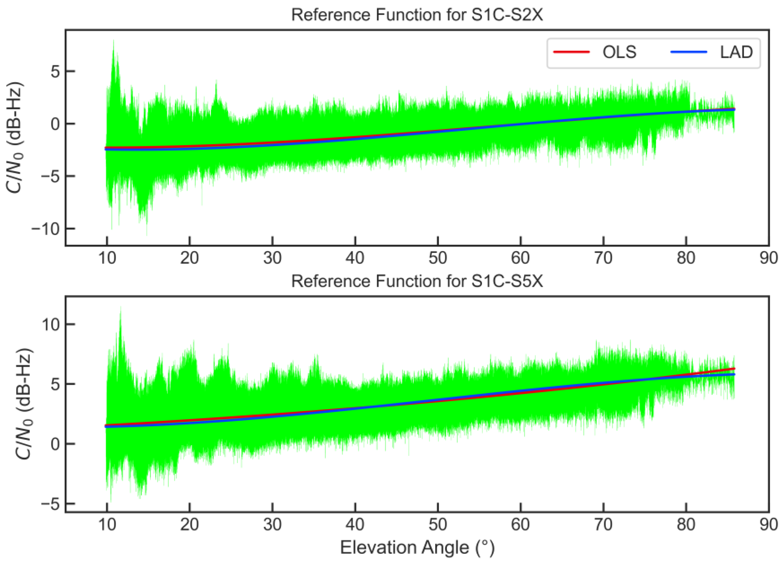
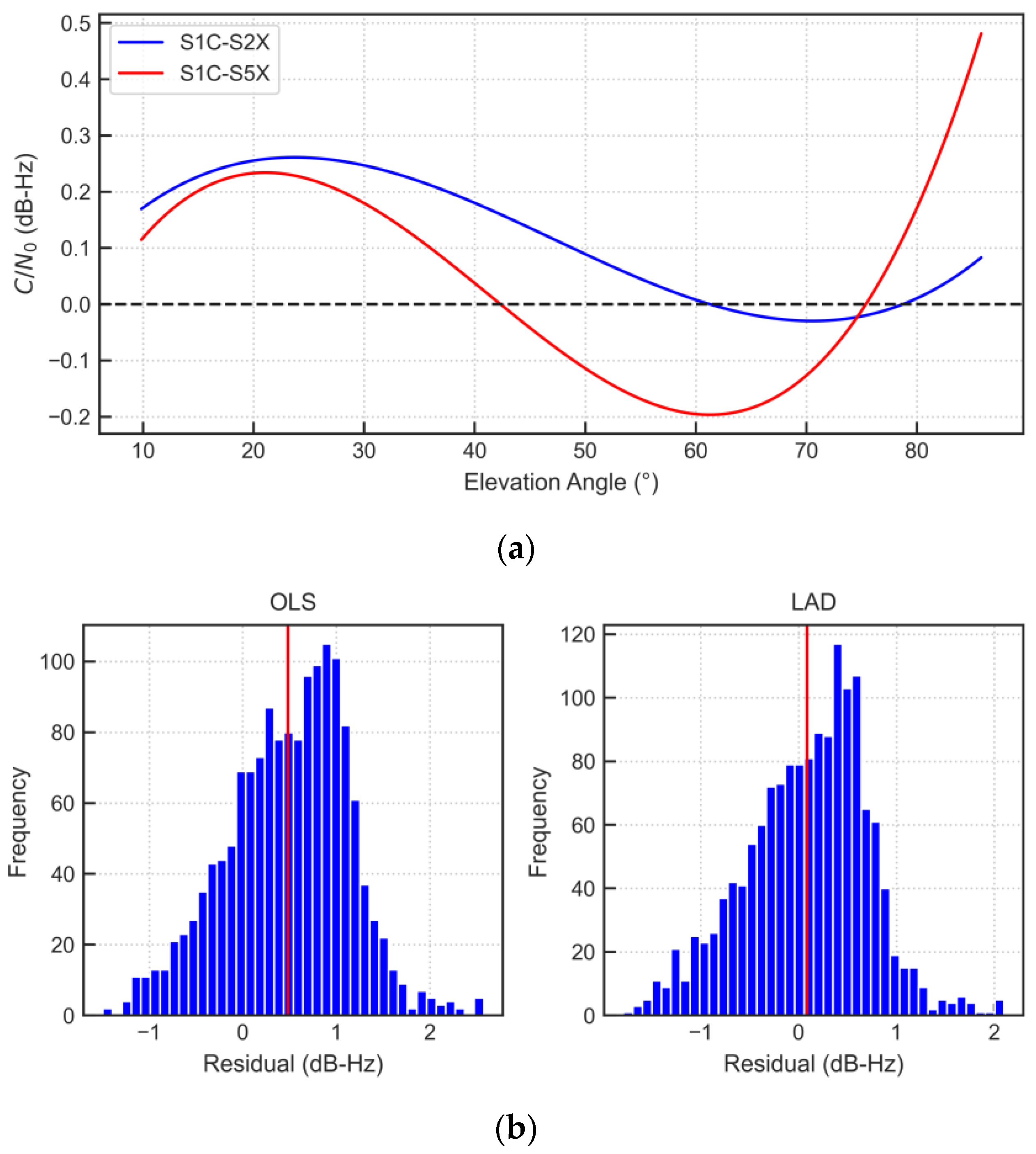
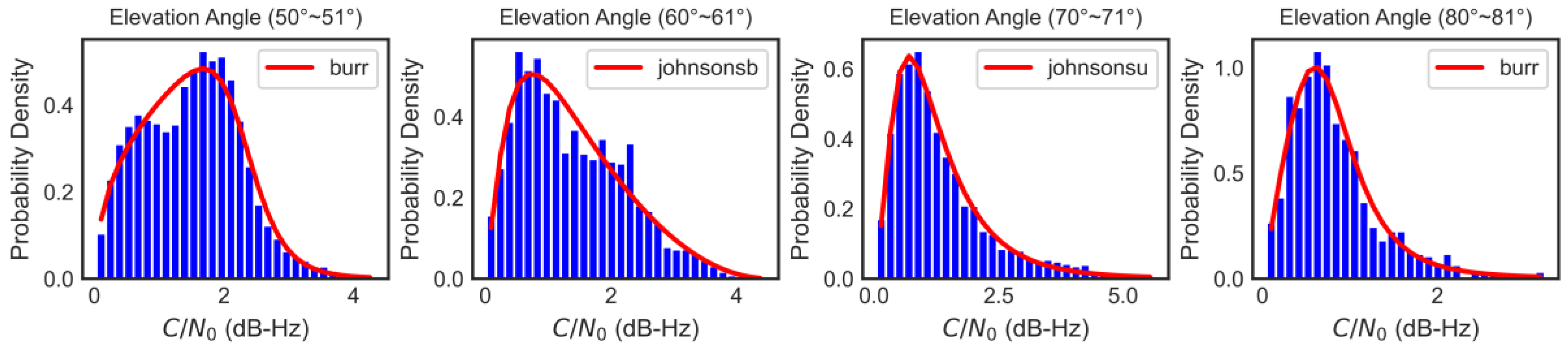
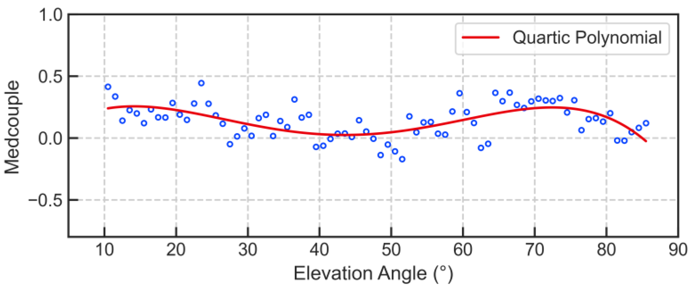
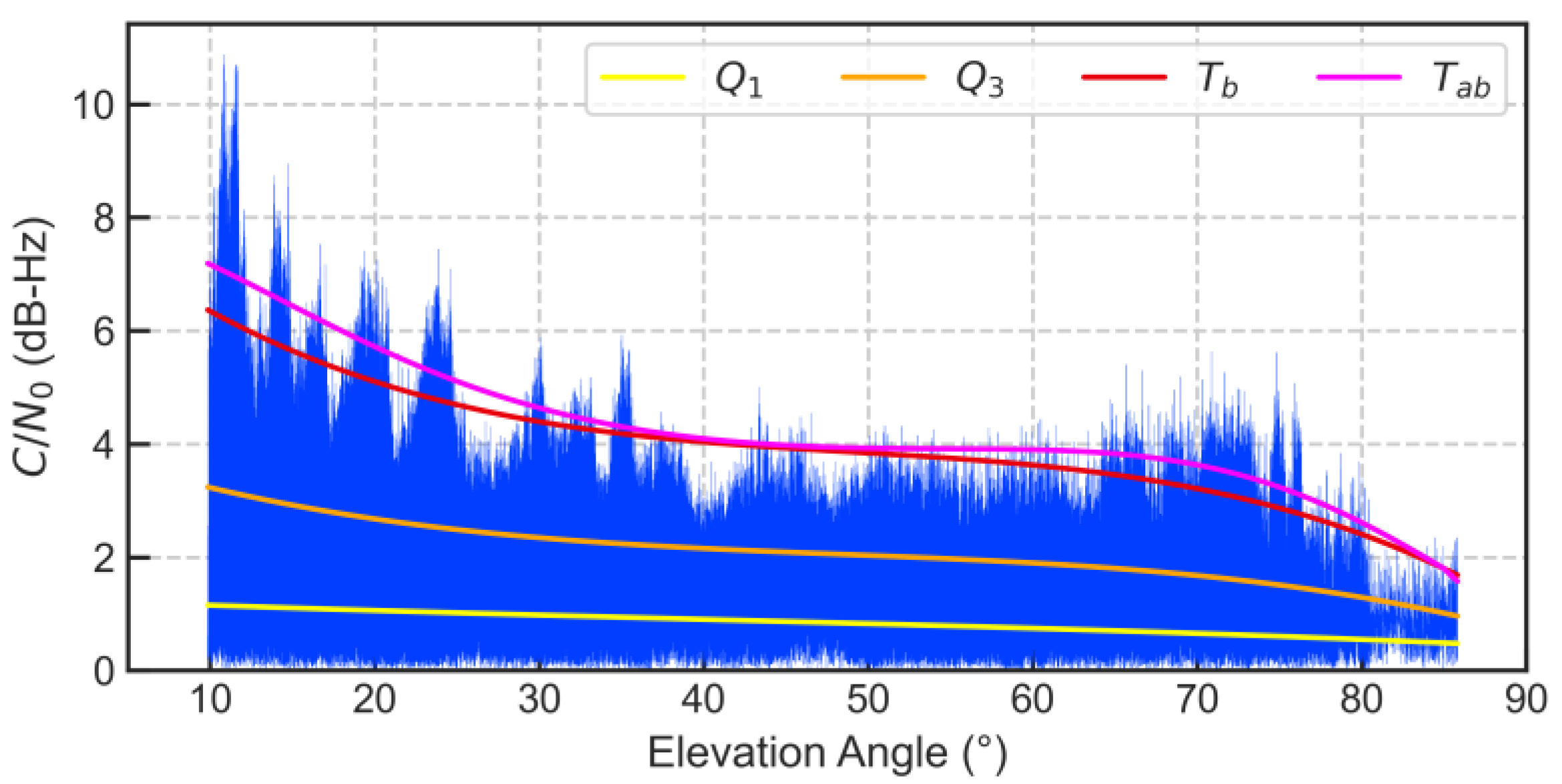
3.1. Modeling of Reference Functions Based on LAD

To calibrate the multipath detector for a specific receiver and antenna, GNSS observations need to be collected in a low-multipath environment. The acquisition site of the static calibration data was on the roof of the Transportation Building at Southeast University in China, where there were no shielding objects around. The types of the receiver and antenna were Trimble BD990 and South CR3, respectively. In addition to GPS, the receiver also supports three-frequency observations of BDS, GLONASS and Galileo. This article only uses GPS observations for research. The cut-off elevation of the receiver was set to 10° to ensure the quality of the data. Finally, 24 h of GNSS three-frequency observations (L1C, L2X and L5X) on October 1, 2019 were obtained with a sampling rate of 1 Hz. The data collection environment and GPS skyplot are shown in Figure 1. Note that the satellite track is not displayed when lock is lost on any frequency.

The function models depending on satellite elevation were established by fitting cubic polynomials for the L1-L2 and L1-L5 C/N₀ differences from all observed GPS satellites in the low-multipath environment. Unlike the classic method, LAD regression was employed to calculate polynomial coefficients in this paper, instead of OLS regression. The developed reference functions are as follows:

$$\Delta C^{12}\left({\theta }_r^s\right)=-1.528\times {10}^{-5}{\left({\theta }_r^s\right)}^3+2.447\times {10}^{-3}{\left({\theta }_r^s\right)}^2-0.057361{\theta }_r^s-2.113$$

(14)

$$\Delta C^{15}\left({\theta }_r^s\right)=-1.257\times {10}^{-5}{\left({\theta }_r^s\right)}^3+1.867\times {10}^{-3}{\left({\theta }_r^s\right)}^2-0.01652{\theta }_r^s+1.417$$

(15)

where ${\theta }_r^s$ is the elevation angle in degrees. Since LAD is robust, some extra preprocessing operations on the calibration data can be omitted to avoid distorting the true distribution of the data. Figure 2 shows the reference functions of the L1-L2 and L1-L5 C/N₀ differences, obtained using LAD and OLS, respectively. In general, the higher the elevation angle, the smaller the variance of the inter-frequency C/N₀ difference. It can be seen that there are certain differences between the two types of reference functions, which indicate that the observation residuals of the calibration data are asymmetrically distributed at some elevation angles, mainly due to the abnormal C/N₀ measurements. In this case, it is difficult to achieve optimal parameter estimation using OLS. Figure 3a shows the curve of difference between OLS and LAD regression (OLS minus LAD). We can find that the difference between the reference functions obtained using these two methods can reach a maximum of about 0.5 dB-Hz. Both curves have relatively large absolute values in the low elevation range, where the outliers are more active. In the medium–high elevation range, L1-L5 reference functions also display large differences. Besides, when the elevation angle is greater than 82°, the two reference functions for L1-L5 C/N₀ differences begin to diverge significantly. To illustrate this distinction more clearly, the residual distribution of the L1-L5 C/N₀ difference at an elevation angle above 82° from LAD and OLS was found, as shown in Figure 3b. We can find that the OLS fitting curve deviated greatly from its nominal value due to the influence of outliers in this range, which makes the mean residual far away from zero, reaching 0.48 dB-Hz. In contrast, the average residual of the LAD fitting curve is close to 0, which is only 0.09 dB-Hz. This demonstrates that LAD regression has higher robustness than OLS.

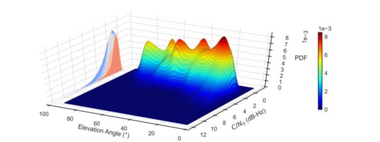
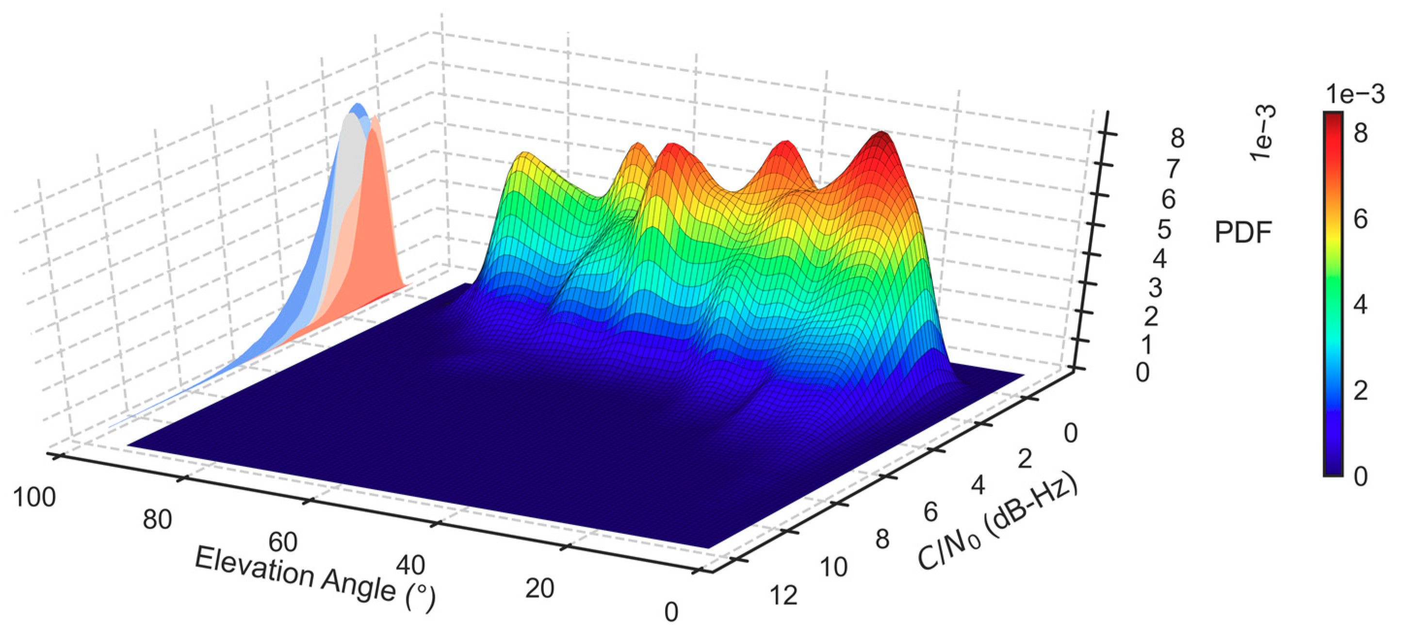
3.2. Distribution of Detection Statistics

The multipath detection statistic was then calculated using Equation (1). To obtain the robust detection threshold, the distribution pattern of $S$ must be analyzed. Figure 4 depicts the joint probability density of the statistics and elevation angle, which was estimated using Gaussian kernels. Its projection on the C/N₀–probability density function (PDF) plane is approximately the probability distributions of $S$ at five specified elevation angles. These statistics present a non-Gaussian distribution. The joint probability density surface demonstrates that the statistics for all elevation angles are generally skewed data. Consequently, the 3σ rule based on the mean and standard deviation cannot provide a reliable threshold model.

The distributions of $S$ at eight typical elevation ranges with an interval of 1 degree are further given, as shown in Figure 5, and their optimal probability densities are fitted. The detailed statistical parameters are listed in

Table 1. Statistical parameters of S at eight elevation ranges with 1-degree interval.

Elevation Range (°)	Sample Size	Skewness	Kurtosis	Mean (dB-Hz)	Median (dB-Hz)	Kolmogorov–Smirnov Test Statistics
10~11	4356	1.302	0.979	2.745	2.017	0.690
20~21	7576	1.207	1.619	1.762	1.517	0.595
30~31	4599	0.944	1.012	1.667	1.573	0.597
40~41	3519	−0.043	−0.565	1.511	1.540	0.638
50~51	5720	0.262	−0.238	1.509	1.546	0.588
60~61	2428	0.630	−0.247	1.384	1.219	0.566
70~71	2269	1.377	1.734	1.317	1.047	0.564
80~81	882	1.410	2.517	0.837	0.724	0.539

, as well as the normality test results of the data using the Kolmogorov–Smirnov (KS) test. After calculation, all KS test P-values are infinitely close to 0, so they are not listed in the table. In statistics, skewness measures the asymmetry of the probability distribution of a random variable relative to the mean value. For a unimodal distribution, negative skewness usually means the tail is on the left of the distribution, while positive skewness means the tail is on the right. The skewness of normally distributed data is about zero. Kurtosis, often referred to as excess kurtosis, is a measure that reflects the steepness or smoothness of the data distribution. A higher kurtosis generally indicates a heavier tail. The kurtosis of the normal distribution is regarded as zero. The results of the KS test are another reference. When the P-value is less than the significance level of 0.05, the null hypothesis is rejected, that is, the data are considered not subject to normal distribution. We can see that these sets of statistics are very inconsistent with the normal distribution. Specifically, except for statistics at elevation range (40°, 41°), the rest are right-skewed data, in which the skewness of statistics at elevation range (10°, 11°), (20°, 21°), (70°, 71°) and (80°, 81°) is even greater than 1. There also appear to be five groups of statistics that show varying degrees of heavy-tailed distribution. In addition, the data at elevation range (10°, 11°), (30°, 31°), (50°, 51°), (60°, 61°) and (80°, 81°) all present some degree of bimodal distribution. The above statistical characteristics weaken the effect of the 3σ rule in judging outliers of these data.

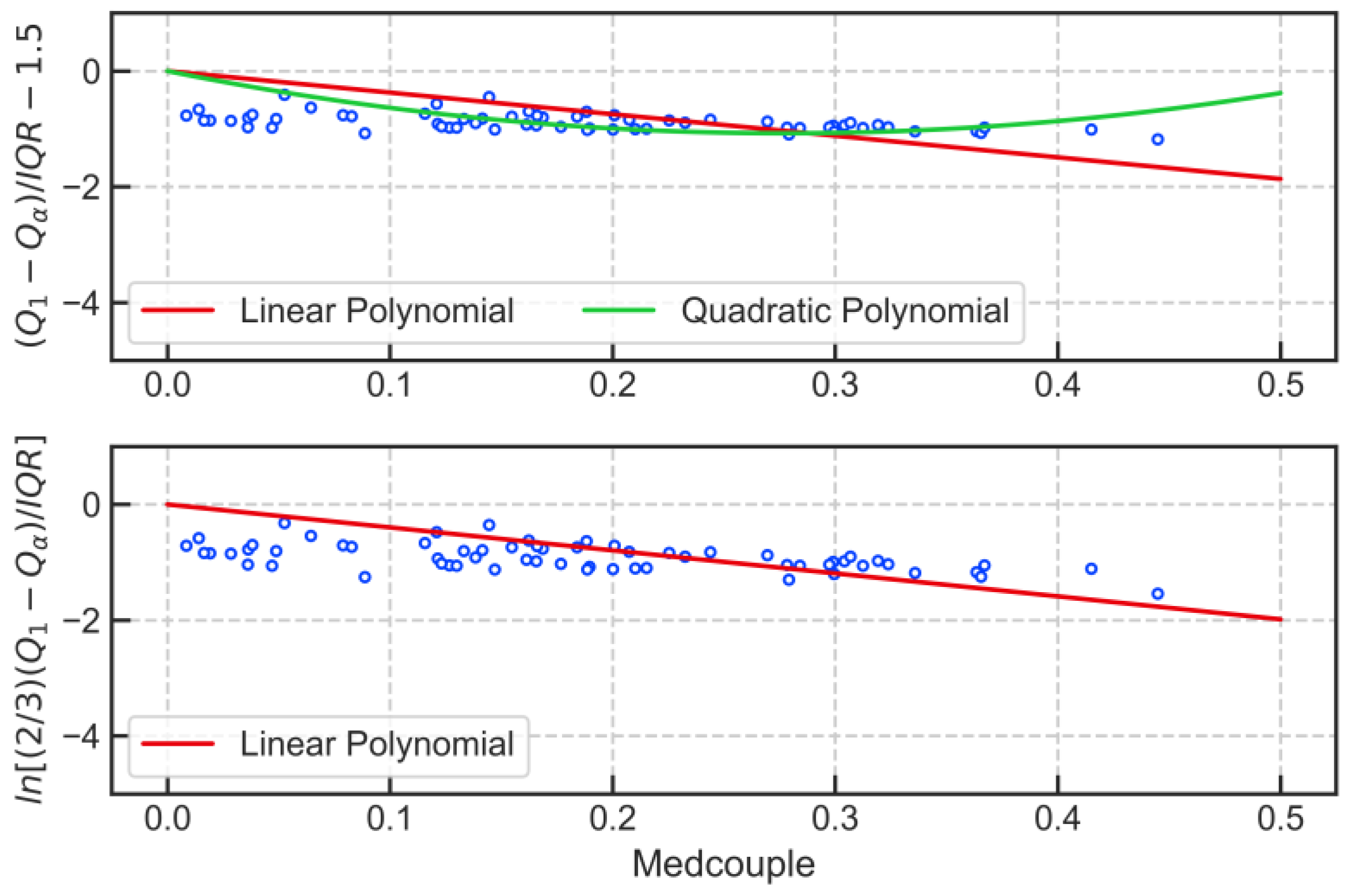
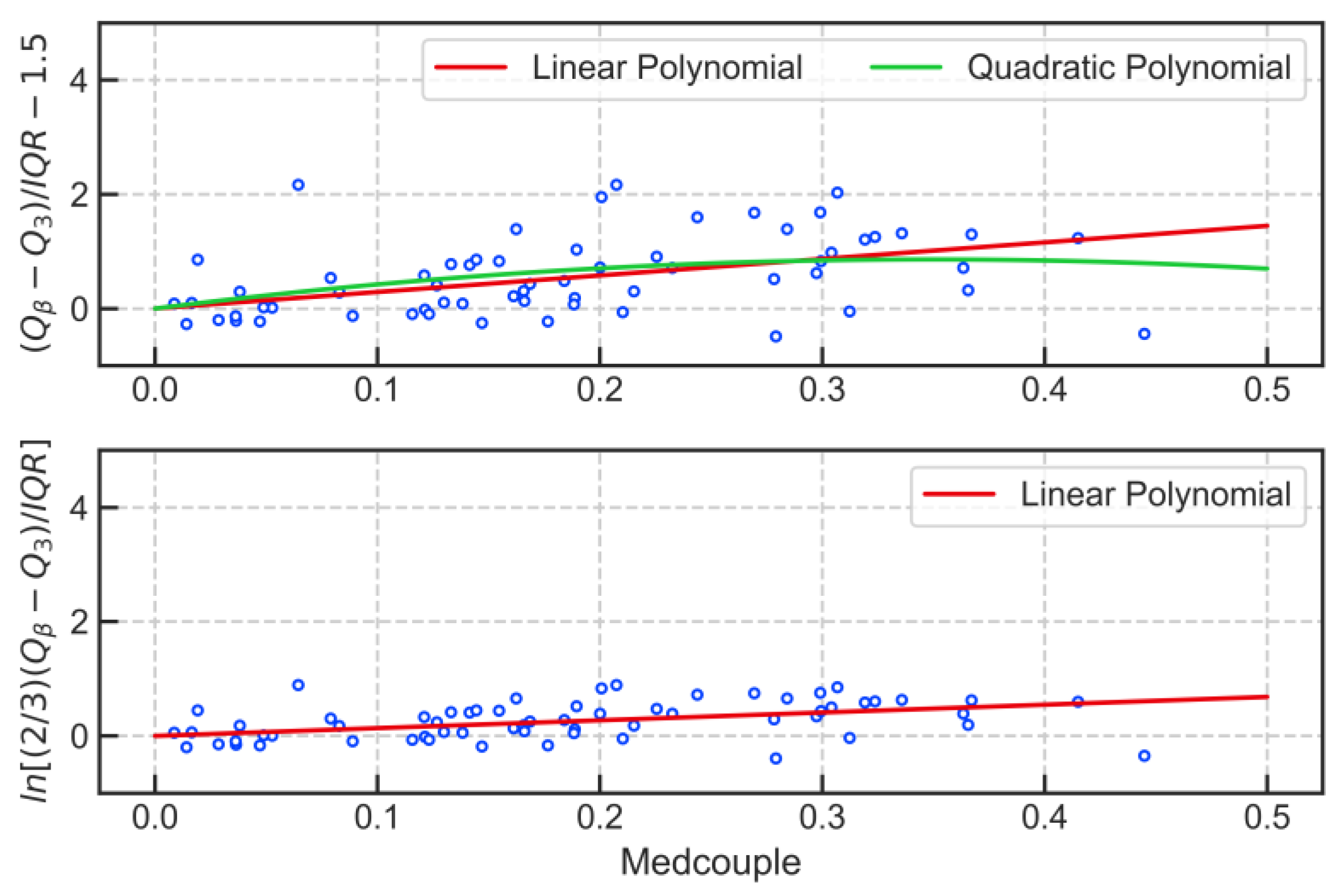
3.3. A Robust Multipath Detection Method for Skewed Data

The skewness parameter of the sample data depends on the second and third empirical moments, which are very sensitive to outliers. Therefore, a more robust parameter, medcouple (MC), is used to measure the asymmetry of the data. It is defined as [34]

$$MC=\underset{x_i\le Q_2\le x_j}{\mathrm{med}}h\left(x_i,x_j\right)$$

(16)

where $Q_2$ is the median of the samples; for all $x_i\ne x_j$, the kernel function $h$ is given by

$$h\left(x_i,x_j\right)=\frac{\left(x_j-Q_2\right)-\left(Q_2-x_i\right)}{x_j-x_i}$$

(17)

Brys et al. [34] also gave a specific definition for the special case $x_i=Q_2=x_j$, even though the probability of its occurrence is almost zero. By definition, the value of MC is between −1 and 1. The MC of right-skewed data is positive, and the MC of left-skewed data is negative. It has a bounded influence function and a breakdown value of 25%, which means that at least 25% outliers are needed to make MC reach 1 or −1.

To obtain the robust outlier boundary of skewed data, two functions related to MC were introduced into the standard boxplot to replace the constant 1.5. The adjusted fence is therefore defined below [25]:

$$\left[Q_1-h_l\left(MC\right)IQR, Q_3+h_u\left(MC\right)IQR\right]$$

(18)

where $h_l\left(0\right)=h_u\left(0\right)=1.5$ is required to determine the outlier threshold of symmetric distributions. The following three simple models for $h_l$ and $h_u$ were considered:

(1) linear model:

$$\{\begin{array}{c}{h}_l\left(MC\right)=aMC+1.5\\ h_u\left(MC\right)=bMC+1.5\end{array}$$

(19)

(2) quadratic model:

$$\{\begin{array}{c}{h}_l\left(MC\right)=a_{1}M{C}^2+a_{2}MC+1.5\\ h_u\left(MC\right)=b_{1}M{C}^2+b_{2}MC+1.5\end{array}$$

(20)

(3) exponential model:

$$\{\begin{array}{c}{h}_l\left(MC\right)=1.5e^{aMC}\\ h_u\left(MC\right)=1.5e^{bMC}\end{array}$$

(21)

where $a, b, a_1, a_2, b_1, b_2\in \mathbb{R}$.

In order to solve the coefficients of the above functions, the expected percentage of outliers is set to be close to 0.7%, which is in accordance with the proportion of outliers in the standard boxplot under a normal distribution. Therefore, the left and right fence boundaries in Equation (18) must satisfy:

$$\{\begin{array}{c}{Q}_1-h_l\left(MC\right)IQR\approx Q_{\alpha }\\ Q_3+h_u\left(MC\right)IQR\approx Q_{\beta }\end{array}$$

(22)

where $Q_{\alpha }$ and $Q_{\beta }$ are the $\alpha$th and $\beta$th percentile of the distribution, $\alpha =0.0035$ and $\beta =0.9965$.

By substituting Equations (19)–(21) into Equation (22), the three models can be converted into:

$$\{\begin{array}{c}\frac{Q_1-Q_{\alpha }}{IQR}-1.5\approx aMC\\ \frac{Q_{\beta }-Q_3}{IQR}-1.5\approx bMC\end{array}$$

(23)

$$\{\begin{array}{c}\frac{Q_1-Q_{\alpha }}{IQR}-1.5\approx a_{1}M{C}^2+a_{2}MC\\ \frac{Q_{\beta }-Q_3}{IQR}-1.5\approx b_{1}M{C}^2+b_{2}MC\end{array}$$

(24)

$$\{\begin{array}{c}\ln \left(\frac{2}{3}\frac{Q_1-Q_{\alpha }}{IQR}\right)\approx aMC\\ \ln \left(\frac{2}{3}\frac{Q_{\beta }-Q_3}{IQR}\right)\approx bMC\end{array}$$

(25)

The linear regression without intercept can be used to estimate parameters. In order to find the best model, we divided the statistic $S$ with a 1-degree elevation interval and calculated the MC values. These data subsets follow different distributions and are skewed variously, which is conducive to function fitting. Here, we only considered the symmetric and right-skewed distributions, because for the left-skewed data, the boxplot fences just need to be flipped. Therefore, we selected the data subsets with MC ≥ 0 and computed their values on the left side of the equal sign in the above three models. The fitted curves for the lower and upper boundaries using OLS regression of the linear, quadratic and exponential model are shown in Figure 6 and Figure 7, respectively. From Figure 6, the fitting effect of the linear and exponential model is better than that of the quadratic model for the lower boundary. Figure 7 further demonstrates the superiority of the exponential model over the linear model for the upper boundary.

For the sake of model simplification and robustness, we rounded down the estimated values of exponential model coefficients $a=-3.97$ and $b=1.34$ to $a=-4$ and $b=1$. Since MC is susceptible to a large proportion of outliers, when the calibration data are not clean enough (as is often the case), the MC estimate may be biased towards outliers, which will result in an excessively large fence. To reduce the potential false negative rate and make the model more robust, we lowered the estimates of $a$ and $b$. Thus, the outlier boundaries of skewed data were obtained. Considering that the mathematical meaning of the statistic $S$ is the deviation of C/N₀ differences from their reference functions, it has only a one-sided (right-sided) outlier boundary. The robust boxplot fence for skewed statistics is

$$T_{ab}=\{\begin{array}{c}{Q}_3\left({\theta }_r^s\right)+1.5e^{MC\left({\theta }_r^s\right)}IQR\left({\theta }_r^s\right), MC\ge 0\\ Q_3\left({\theta }_r^s\right)+1.5e^{4MC\left({\theta }_r^s\right)}IQR\left({\theta }_r^s\right), MC<0\end{array}$$

(26)

where the second formula is obtained by flipping the lower boundary in the first case.

The polynomial of degree 4 was then used to fit the MC values from the data subsets, as shown in Figure 8, and the MC function related to elevation angle was obtained as follows:

$$MC\left({\theta }_r^s\right)=-3.151\times {10}^{-7}{\left({\theta }_r^s\right)}^4+5.465\times {10}^{-5}{\left({\theta }_r^s\right)}^3-3.020\times {10}^{-3}{\left({\theta }_r^s\right)}^2+0.05621{\theta }_r^s-0.07683$$

(27)

The first and third quantile functions for the statistics can be obtained by using quantile regression:

$$Q_1\left({\theta }_r^s\right)=-8.664\times {10}^{-7}{\left({\theta }_r^s\right)}^3+1.044\times {10}^{-4}{\left({\theta }_r^s\right)}^2-0.01170{\theta }_r^s+1.264$$

(28)

$$Q_3\left({\theta }_r^s\right)=-1.281\times {10}^{-5}{\left({\theta }_r^s\right)}^3+1.867\times {10}^{-3}{\left({\theta }_r^s\right)}^2-0.1022{\theta }_r^s+4.081$$

(29)

Therefore, the interquartile range function can be written as

$$IQR\left({\theta }_r^s\right)=Q_3\left({\theta }_r^s\right)-Q_1\left({\theta }_r^s\right)$$

(30)

The new multipath detection threshold, which has higher robustness for skewed data, was obtained by substituting Equations (27)–(30) into Equation (26).

Figure 9 shows the multipath detection statistic and robust threshold from the calibration data in the low-multipath environment. Meanwhile, the threshold for the standard boxplot was also given. It can be seen that the adjusted boxplot corrects the standard boxplot fence $T_b$ according to the skewness of the data distribution, especially at the elevation angles of (10°, 30°) and (60°, 80°). The multipath detection threshold based on the standard boxplot can be calculated by the following formula:

$$T_b=Q_3\left({\theta }_r^s\right)+1.5IQR\left({\theta }_r^s\right)=-3.073\times {10}^{-5}{\left({\theta }_r^s\right)}^3+4.511\times {10}^{-3}{\left({\theta }_r^s\right)}^2-0.2380{\theta }_r^s+8.307$$

(31)

In Figure 9 and for comparison, three multipath detection thresholds calculated by the classic method are also given below:

$$T_{\sigma }=-1.028\times {10}^{-5}{\left({\theta }_r^s\right)}^3+1.569\times {10}^{-3}{\left({\theta }_r^s\right)}^2-0.08743{\theta }_r^s+4.295$$

(32)

$$T_{2\sigma }=-1.028\times {10}^{-5}{\left({\theta }_r^s\right)}^3+1.569\times {10}^{-3}{\left({\theta }_r^s\right)}^2-0.08743{\theta }_r^s+5.366$$

(33)

$$T_{3\sigma }=-1.028\times {10}^{-5}{\left({\theta }_r^s\right)}^3+1.569\times {10}^{-3}{\left({\theta }_r^s\right)}^2-0.08743{\theta }_r^s+6.437$$

(34)

The meaning of the above thresholds is the sum of the mean and standard deviation of the statistic. The former is a fitted cubic polynomial, and the latter is a constant value across all elevations, equal to 1.071 dB-Hz. Note that the detection statistic was based on the following reference functions, which were obtained by using OLS:

$$\Delta C^{{12}^{’}}\left({\theta }_r^s\right)=-9.615\times {10}^{-6}{\left({\theta }_r^s\right)}^3+1.646\times {10}^{-3}{\left({\theta }_r^s\right)}^2-0.02891{\theta }_r^s-2.152$$

(35)

$$\Delta C^{{15}^{’}}\left({\theta }_r^s\right)=6.925\times {10}^{-7}{\left({\theta }_r^s\right)}^3+2.294\times {10}^{-4}{\left({\theta }_r^s\right)}^2+0.03482{\theta }_r^s+1.172$$

(36)

The multipath detection statistic and thresholds for the classic method are shown in Figure 10. With reference to Figure 9, it can be seen that $T_{ab}$ better corresponds to the distribution of statistic than $T_{3\sigma }$. Additionally, $T_{ab}$ takes into account the skew of the data. Intuitively, as the elevation angle increases, the multipath detection threshold of $T_{ab}$ becomes increasingly more stringent compared to $T_{3\sigma }$.

4. Performance Verification

In order to verify the performance improvement of the new detector for multipath detection, we collected three sets of GPS three-frequency observations in multipath environments for experiments conducted on 23 October 2019, including two sets of static data and one set of kinematic data. Since the detection statistic $S$ is receiver and antenna dependent, the receiver and antenna used in the experiments are the same as those in the calibration experiment.

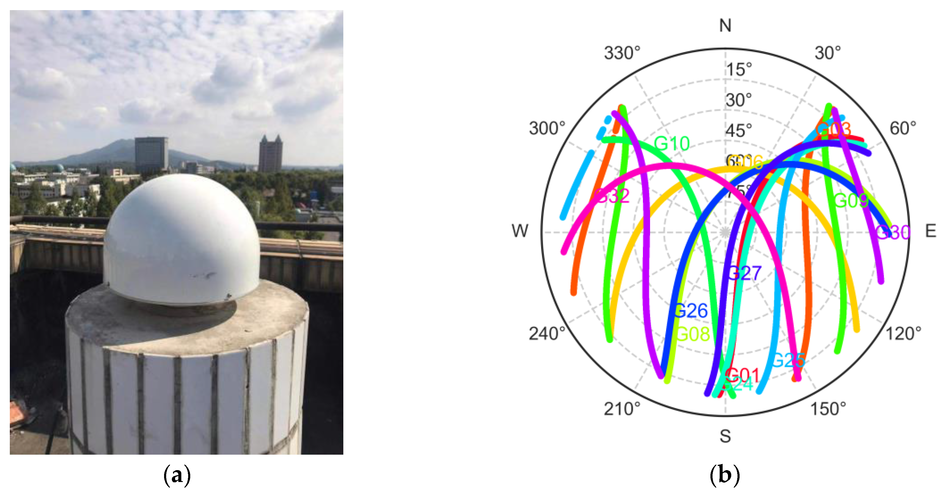
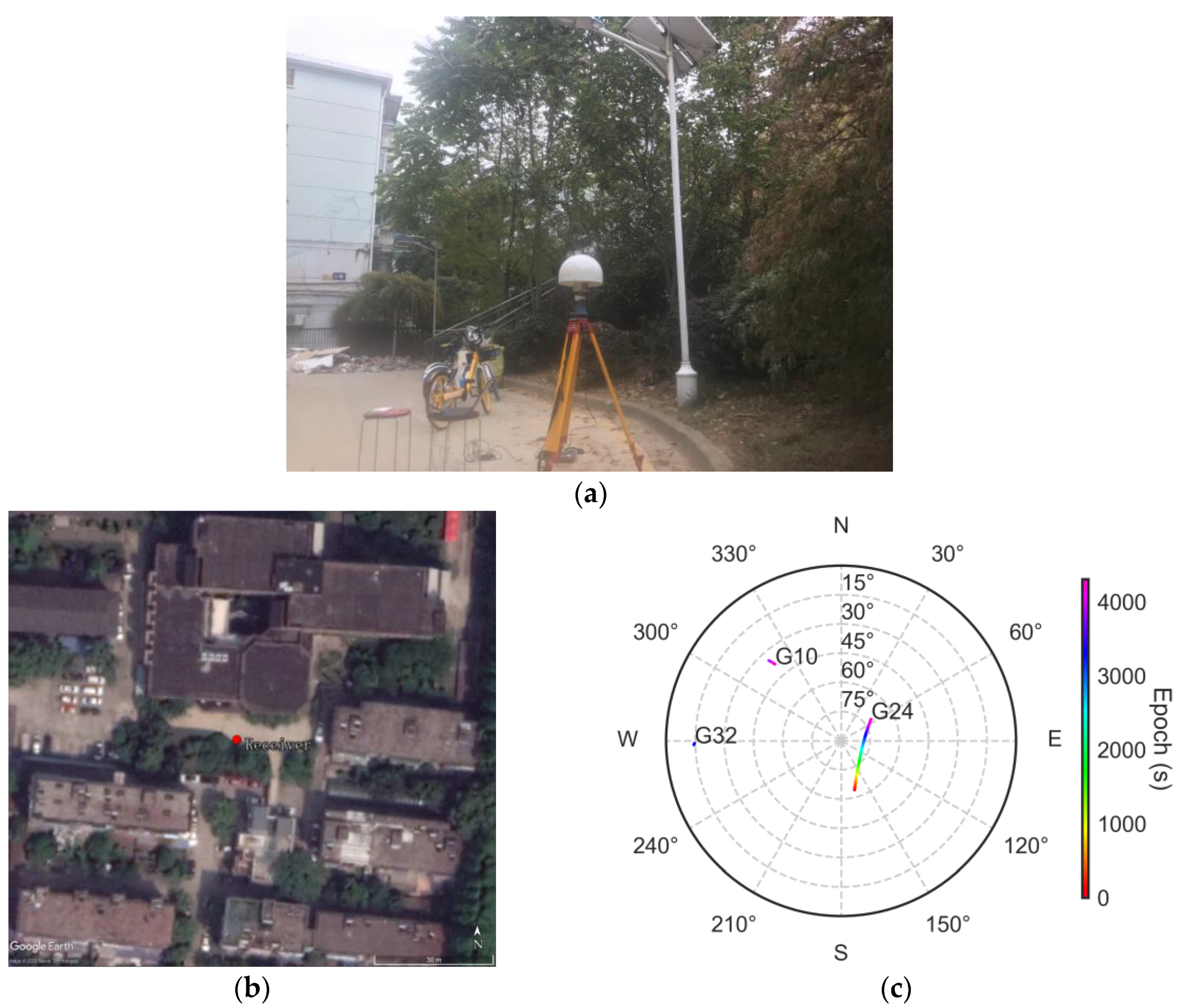
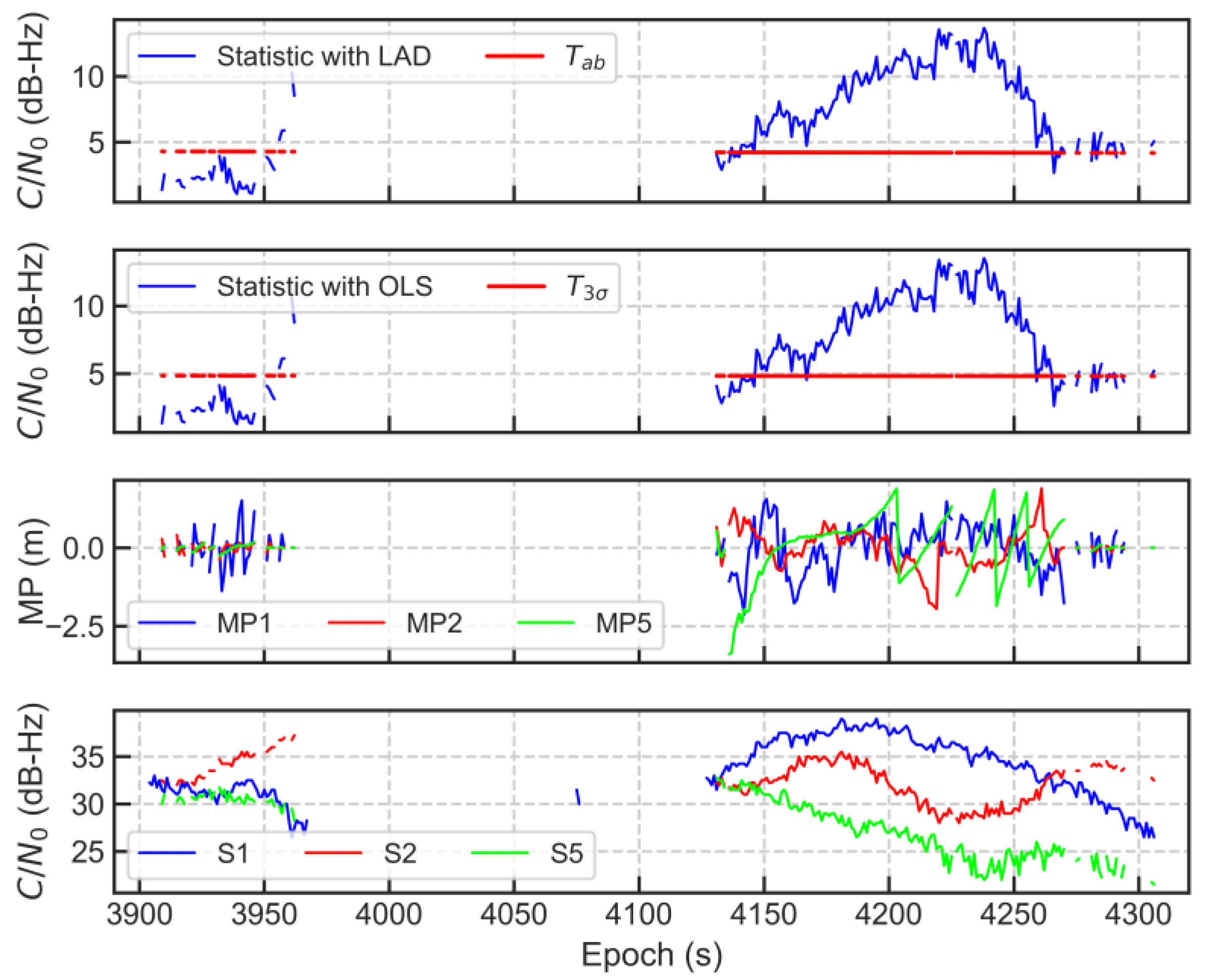
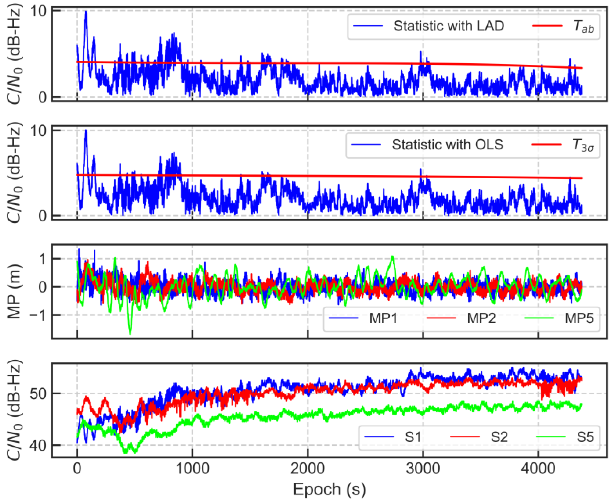
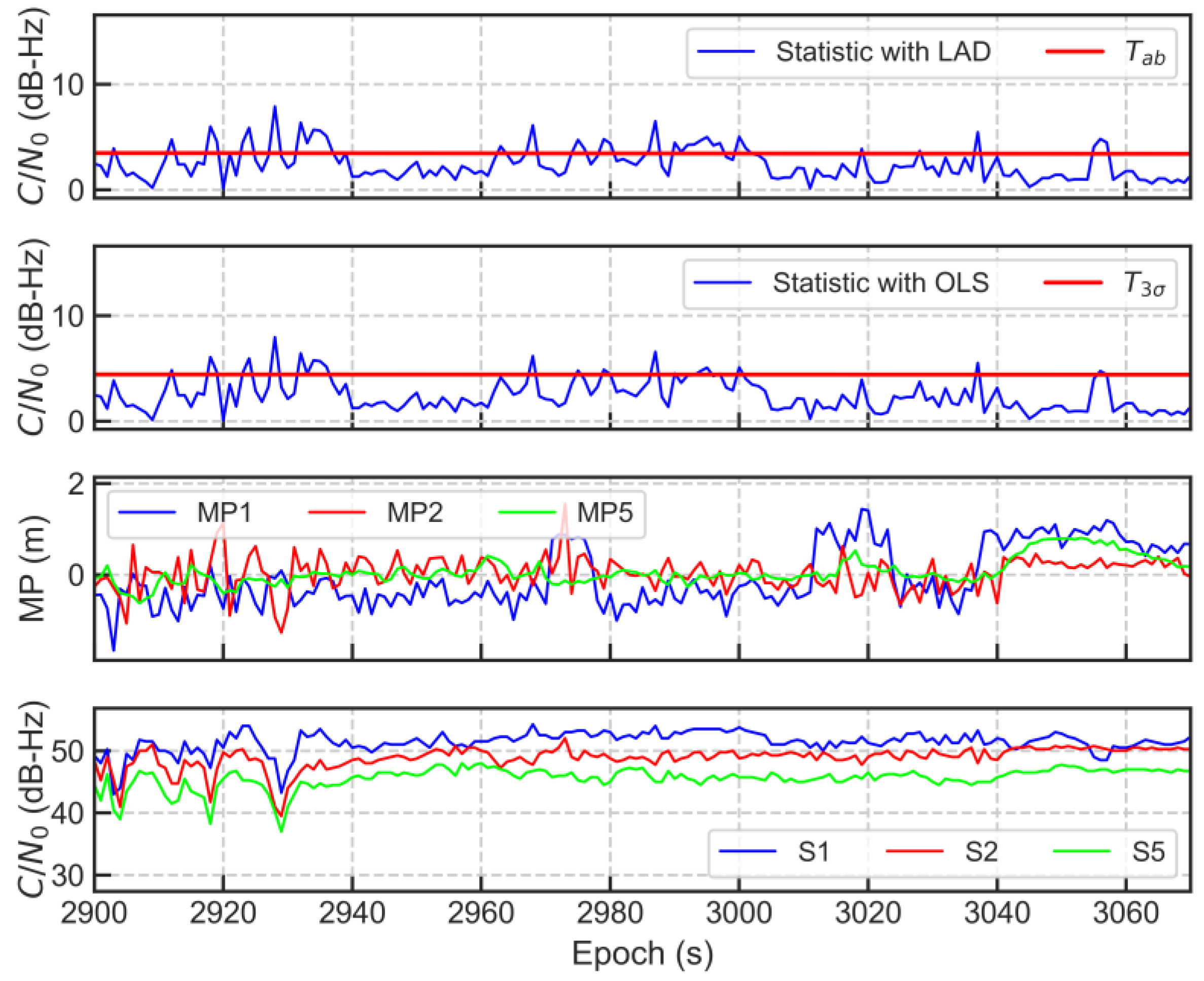
4.1. Static Observation

The static test sites are located in the Western Campus of Southeast University, where most of the buildings have coarse surfaces, so the receiver is vulnerable to diffuse multipath interference. The first observation site is shown in Figure 11a and its aerial view is shown in Figure 11b. The receiver was erected close to the building (about 10–20 m), and some trees around it also seriously obstructed its view of the satellites. Note that the viewing angle of Figure 11a is eastward and slightly to the south. This is a typical diffraction and short-delay multipath environment. Figure 11b depicts the skyplot of GPS observations with the satellite elevation and azimuth changes to facilitate the comparison of the satellite position relative to the environment. Similarly, the satellite trajectory is not displayed when loss of lock occurs on any frequency. It can be seen that only three satellites are tracked during the observation period. Of these, the satellite PRN 24 has the longest data acquisition time.

Figure 12 shows the multipath detection results for PRN 24. The subgraphs from top to bottom represent the new adjusted boxplot detection method, the classic 3σ detection method, three-frequency code multipath observables and the absolute C/N₀ measurements, respectively. Both detectors are presented at the same time for comparison. Due to the high elevation angle of the satellite, the amplitude of the MP observables is small and the detection statistic ranges from 0 to 5 dB-Hz. The oscillation of the MP values reflects that the satellite signals may be affected by multiple reflections. Nevertheless, the new detection method is more sensitive to multipath and diffraction at high elevation angles (about above 65°). Typically, the MP values show relatively large variations between 2400 and 2600 s and around 3200 s, when the detection statistics from the new method are significantly above the threshold. Besides, the change in MP2 value between 3800 and 4000 s is also detected by the new method, while the classic method has the multipath omission. In such an environment partially covered by trees, diffraction is very frequent, but the MP value often cannot reflect this interference. By observing the surrounding obstructions and skyplot, we can find that PRN24 is susceptible to interference by the diffraction signal before 3000 s, and the new method is more sensitive to this.

The multipath detection results of PRN 10 at medium elevation angles (about 32°–36°) were also analyzed. From Figure 13, the magnitude of the change in MP values has become significantly larger. Tracking interruption occurs between 3970 and 4130 s. Besides, the receiver resets frequently between 3900 and 3970 s and after 4270 s. Discontinuous observations indicate a complex acquisition environment. There is a distinct oscillation in MP1 values between 3920 and 3950 s. However, the detection statistics do not respond to this. The reason may be that the multipath detection method based on the inter-frequency C/N₀ difference is sensitive to short-delay multipath, while the MP value is sensitive to medium-delay multipath. The environment in which the receiver is located also demonstrates that the multipath is mainly due to short delay. A large statistic jump occurs around 3960 s, which exceeds the threshold, but there is not much change in the MP values at the corresponding time. Given the receiver reset during this period and subsequent tracking interruption, this indicates that the satellite signal is likely to be diffracted. The absolute C/N₀ measurements also prove this. The C/N₀ values of L1 and L5 frequencies attenuate at this time. After being blocked by an obstacle for about 160 epochs, the satellite is re-captured around 4130 s. Note that the detection statistic can catch the diffraction effect, but the MP value cannot. Between 4130 and 4270 s, the MP values show large oscillations, and the detection statistic also greatly exceeds the threshold. It is worth mentioning that, however, the new method detects multipath earlier than the classic method, and completely detects the entire multipath along with the MP variations.

The second collection site for static data is slightly further away from the buildings and not close to the trees. Figure 14 shows the real environment around the receiver, aerial view and the skyplot of three-frequency observations. The perspective of the real environment photo is towards the southeast. The observation environment is a bit more open than the first site, and there are three GPS satellites that have been observed for a long time. Here, the observation times for satellites PRN 10 and PRN 24 are almost identical and correspond to a little more than an hour of continuous observation. Notice that the receiver is close to a car and may be interfered by the specular reflection signal.

The multipath detection results of the PRN 10 satellite are shown in Figure 15. The satellite is in a phase of ascending elevation. Over the first 900 s, the MP values show relatively large oscillations. Compared with the classic detection method, the new detection method is more sensitive to the multipath during this observation period. After 900 s, for both methods, the statistic does not significantly exceed the threshold according to the MP variations. This may be because the detection statistic based on C/N₀ is more sensitive to short-delay multipath. The environment in which the receiver is located can cause more medium-delay multipath to be received. This may also be a problem of greater attenuation caused by NLOS signal for larger MP variations. However, the multipath at the end of the observation period (around 4300 s) is still captured by the new detector.

Figure 16 shows the multipath detection results of the PRN 24 satellite. As the elevation angle decreases, the absolute C/N₀ measurements attenuate and the magnitude of the MP variations becomes larger. The corresponding detection statistic also increases and gradually exceeds the threshold. Although the sensitivity of the detection statistic to short-delay multipath makes it unable to fully correspond to the MP variation in this environment, and results in the magnitude mismatch between them, the new detector is undoubtedly better in sensitivity to multipath at this elevation scope. The classic method is likely to have a higher risk of false negatives for multipath according Figure 9 and Figure 10. The detection statistic of the new method exceeds the threshold around 630 s, 700 s, 1350 s, 1500 s, 2010 s, 2710 s and 3350 s, and the corresponding MP value changes significantly. However, the classic method does not detect the multipath at these times.

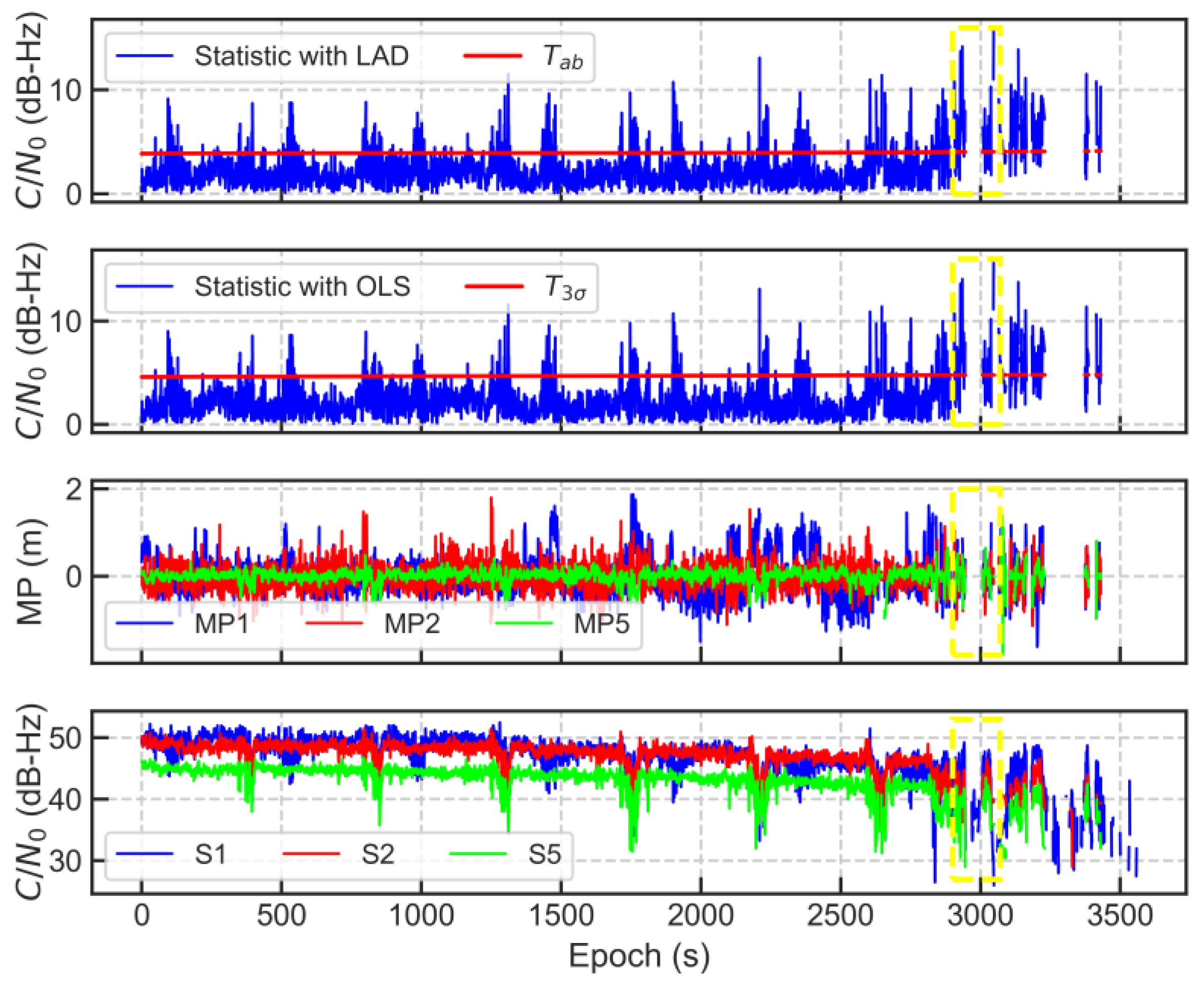
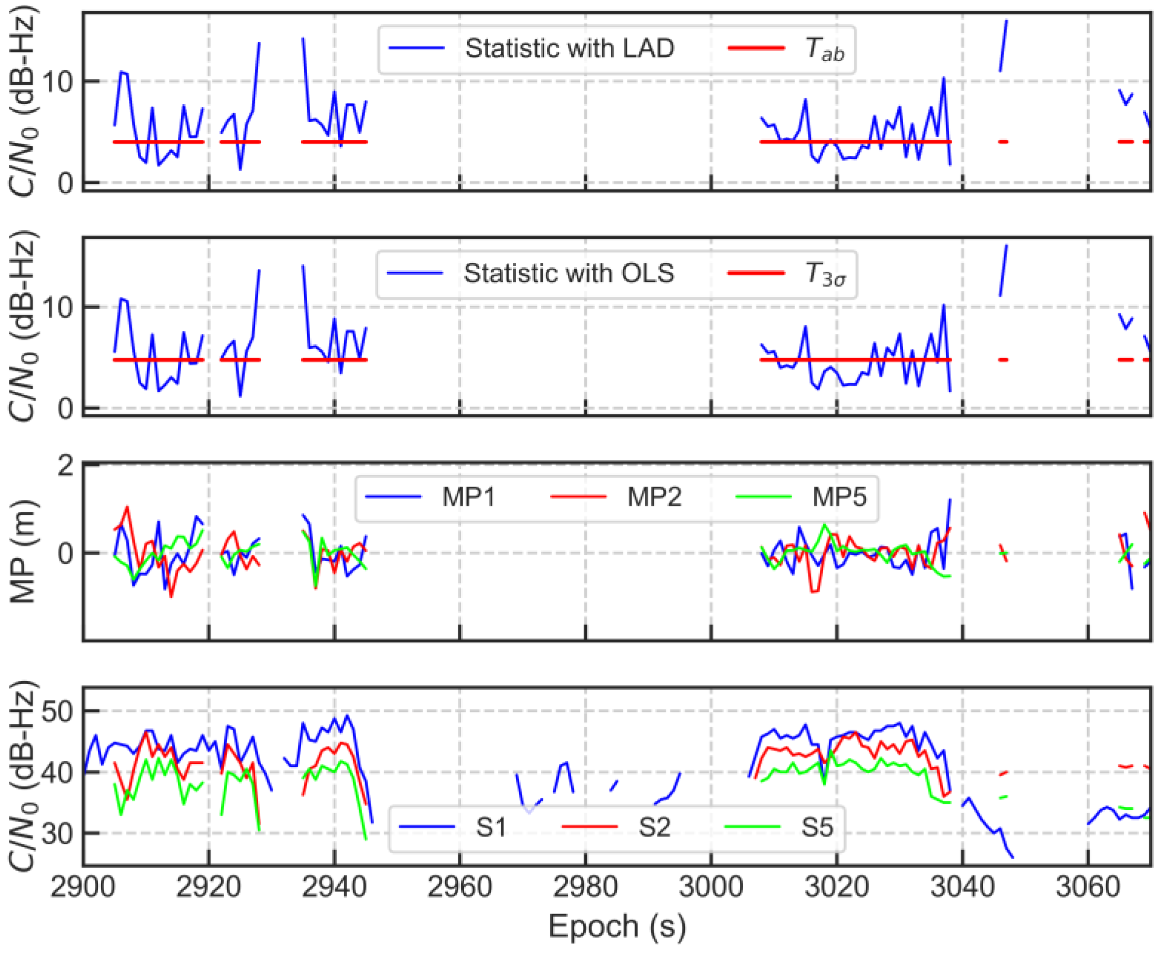
4.2. Kinematic Observation

Although the C/N₀-based multipath detector is more suitable for geodetic applications, the kinematic experiment was still carried out to test the improvement of the new method in multipath detection accuracy. Figure 17 shows the test route and the skyplot of the corresponding observations. In the left panel, the green dot represents the starting point and the yellow dot represents the end point. The receiver and antenna were fixed on a trolley, which was pushed by the experimenters at a normal walking speed. The experimenters first walked around the playground about six times, and then crossed the boulevard back to the Transportation Building. During the period, the experimenter also passed through some buildings. Note that the playground track is surrounded by tall sycamore trees, and there are buildings nearby in all four directions. The overall observation environment is more complicated than the static experiments. The satellite with the longest observation time and the best continuity is PRN 26, followed by PRN 32. Therefore, these two satellites were selected for analysis.

The results of the detection statistic for PRN 26 are shown in Figure 18. From the MP values, the magnitude and frequency of oscillation indicate that the environment is challenging. Data were collected on the playground over the first 2800 s. Starting from 2800 s, the experimenters left the playground and entered the boulevard. Detection statistics, MP values and absolute C/N₀ measurements all show the periodicity of receiver movement on the playground track. In the playground phase, the detection statistic exceeds the threshold at 90–200, 500–720, 960–1160, 1350–1490, 1890–1940 and 2280–2470 s, which is confirmed by the corresponding MP variations. Besides, the large attenuation of the absolute C/N₀ measurements usually means NLOS reception. The amplitude of the MP values confirms this. The peaks in the detection statistic may result from the reception of multiple reflected signals. After leaving the playground, the receiver entered the boulevard, and the observation environment was even worse. The detection statistic goes beyond the threshold more significantly. The magnitude of MP variation also demonstrates that the multipath interference is more serious during this period. There are three large attenuations in the absolute C/N₀ measurements, indicating NLOS reception. It is worth mentioning that between 2900 and 3070 s, the experimenters went out of the boulevard and walked between two buildings and then along trees before entering the boulevard again. The absolute C/N₀ measurements return to stability, albeit with a lag. The detection statistic is also a little bit smaller, as shown in Figure 19. Nevertheless, multipath interference is still detected due to the obstruction of buildings and trees. In addition, for large MP changes occurring around 2975 s, 3019 s and 3037 s, the statistic of the new method is more obvious than that of the classic method when the threshold is exceeded.

In general, the new method is more sensitive to multipath in this tracking period. By associating with the MP variations, we found that the multipath is missed by the classic method at some moments, or the part beyond the threshold is not as significant as the new method.

Figure 20 illustrates the results of the detection statistic for PRN 32. It can be clearly seen that before 2800 s, the four indicators behave a similar periodicity to the PRN 26 satellite, but the phase changes. Besides, with the decrease in the elevation angle and the deterioration of the observation environment, the data are interrupted several times after 2900 s. As can be seen from the indicators in the figure, the satellite is interfered by multiple reflected signals at several time periods. Note that between 2900 and 3070 s, PRN 32 behaves differently from PRN 26. As shown Figure 21, from 2900 to 2945 s, as the receiver enters between the corridor made by the two buildings, the detection statistic exceeds the threshold significantly and the data are interrupted, indicating that the signal is subject to multipath interference. Subsequently, the satellite signal is blocked by the building to the south. After 3008 s, the signal is reacquired until the receiver enters the boulevard again. The four indicators at 2945 s and 3008 s suggest that diffraction is likely to occur from the edge of the building.

The detection statistic responds well to the MP variations, especially at some significant nodes. This could be because the majority of multipath is short delay in the observation environment. Moreover, diffraction may occur frequently in the complex environment, and the signal interference from multiple diffraction sources will cause more short-delay multipath. Similar to PRN 26, the new multipath detector reduces the false negative rate of multipath for PRN 32, which appears more reasonable in such a challenging environment.

5. Discussion

For GNSS precise positioning, three basic multipath mitigation techniques can be generally summarized, i.e., antenna design, signal processing and measurement processing [3]. The first two methods, with their high hardware requirements or computational complexity, are not friendly to low-cost receivers and location-based services (LBS) applications. Additionally, most signal processing-based multipath mitigation solutions cannot handle short-delay multipath and NLOS reception [2,13], whereas multipath in reality is often of the close-range and short-delay type. Measurement-based methods are widely used in the field of geodesy. In addition to weighting based on C/N₀ or elevation angle to reduce the impact of potential multipath on positioning accuracy, the most well-known methods are probably sidereal filtering [35] and hemispherical models [36,37], which model the carrier multipath errors for static observation stations in advance based on the periodicity of satellite motion. However, the application scenarios of measurement-based methods are limited, and they are usually insufficient in real-time and kinematic performance. Some researchers employ external sensors or spatial data to assist in detecting and mitigating multipath or NLOS signals, including infrared cameras, 3D urban building models and light detection and ranging (LiDAR) point clouds [38,39,40]. Despite the improved positioning accuracy, it is expensive to establish and maintain accurate spatial models, and the use of external sensors and data places high demands on the performance of computing equipment. Accurate and instant multipath detection is a prerequisite for reasonable treatment of multipath-contaminated measurements according to different application scenarios, such as correction, exclusion or down-weighting. In addition to accuracy and reliability, computing cost and real-time performance are also important indicators to evaluate multipath detection techniques. In this regard, the emerging machine learning-based methods seem to have the upper hand. In recent years, numerous studies have begun to focus on machine learning or deep learning to identify NLOS/multipath. These methods can reduce the operating cost of traditional methods and improve usability by constructing a mapping relationship between multiple feature parameters and GNSS signal categories, and obtain satisfactory results [6,41,42,43]. To decrease the dependence on external sensors and observation information, a technique for detecting abnormal GNSS observations including multipath and NLOS based on unsupervised learning has also been proposed [44], which shows better performance than traditional receiver autonomous integrity monitoring (RAIM) and cut-off methods. While both can be used for real-time multipath detection, machine learning-based and multi-frequency C/N₀ measurement-based methods have their pros and cons.

Just as the detection methods based on inter-frequency C/N₀ differences require aforehand calibration of the receiver and antenna, the machine learning-based methods (usually referring to supervised learning) need to label the training data in advance. But the costs are quite different. It is always expensive to obtain a labeled dataset that is accurate and can represent all types of states. The current mainstream LOS and NLOS labeling method is based on the 3D building model, which is not only limited by the accuracy and timeliness of 3D building models but also requires the accurate position of the receiver to obtain the correct classification label. The ray-tracing approach based on the 3D building model can be employed to further determine multipath signals [5,45]. However, this method is computationally expensive and subject to the model accuracy and building materials. In some studies that do not use 3D building models, some external sensors and even manual-assisted labeling are required [46]. For the statistical method, it is only necessary to let the multi-frequency receiver collect more than ten hours of static observation data in an open environment, and the calibration measurement processing also occupies less computing resources compared with the dataset training. On the other hand, the detection methods based on inter-frequency C/N₀ differences are receiver and antenna dependent. Different types of equipment need to be calibrated individually. In machine learning, the feature data derived from the measurements are also affected by the device heterogeneity. Besides, machine learning is restricted by scenarios. The rules learned in one scenario may not necessarily apply to other scenarios. In terms of detection accuracy, that of machine learning should theoretically be higher than that of statistical methods. The univariate-based statistical method is often suboptimal because when the state is determined by only one variable, it cannot be exactly known, especially in complex urban environments [43], unless the state is only determined by this variable and the exact mathematical model between the two is derived. Therefore, as long as the training set label is accurate and the model generalization ability is strong, the performance of the supervised classification model integrating multiple feature values is generally better than the statistical detection method relying only on a single variable. However, how to select appropriate feature variables as the input of the machine learning model is a problem that needs further research.

It must be pointed out that the statistical multipath detector based on the inter-frequency C/N₀ difference is only one of many detection methods, and no single method is completely reliable, so it should be employed in a combined method [13,16]. In view of the complexity and difficulty of multipath detection and mitigation, we still need to resort to more effective comprehensive methods, including, but not limited to, advanced antenna and receiver techniques, measurement processing and even external sensors.

6. Conclusions and Future Work

A robust multipath detection method is proposed in this paper and compared to the classic 3σ method using inter-frequency C/N₀ differences. In the classic method, it is difficult for OLS to resist the influence of outliers on the calibration data, which makes the reference function easily deviate to the outliers. Moreover, because the detection statistics show significant non-negative right-skewed characteristics, the 3σ rule is no longer applicable to the determination of the outlier boundary of these skewed data. A statistical improvement is made to the classical method to make it more robust. Firstly, for the outliers in the calibration data, the reference functions of C/N₀ differences are fitted using LAD to obtain more accurate nominal values. On this basis, the multipath detection statistics are calculated and their distributions are analyzed in detail. The detection threshold is finally obtained by using quantile regression and the adjusted boxplot, which are both deduced explicitly. The new method can dynamically adjust the outlier boundary according to the distribution of detection statistics, which is more in line with the skew characteristics of statistics. Additionally, MC and quantile are more robust than the mean and standard deviation in outlier detection. The performance of this new detection method has been verified statically and kinematically in multipath-prone environments. Compared with the classic method, the new detection method can make a more accurate response to the large change of MP value at most elevation angles. Meanwhile, the satellite diffraction signal can also be accurately detected. The proposed method is more suitable for real-time carrier multipath detection in static and low-dynamic scenarios. It is sensitive to short-delay multipath and is an important supplement to multipath detection techniques.

The research work in this paper provides a more scientific reference for real-time multipath detection using multi-frequency C/N₀ measurements or other statistical data. Nevertheless, there is still room for improvement. First, an individual detector could be set up for each satellite. The C/N₀ differences from different satellites at the same elevation angle are inconsistent. Although this deviation is small for GPS, it is still sufficient to affect the determination of the threshold, so that the threshold cannot fit well with each satellite. Second, it is also a question whether the cubic polynomial is the best model for reference function, as well as for the quantiles of detection statistic. The authors used the default model from the classic method, and perhaps there are better models, such as polynomial models with L¹ regularization, support vector regression model, etc., that could be employed in the future. It is worth mentioning that it is possible to further improve the reliability of this method by using C/N₀ measurements from different channels. In addition, the statistical multipath detection for the different constellations of BDS has yet to be verified.

Our experiments are conducted based on the measured data in real complex environments. Since the true multipath and its magnitude are unknown, the verification process mainly relies on some external relevant indicators. Although the measured data are irreplaceable in authenticity, it has to be admitted that the simulated data do have advantages over the measured data in terms of variable control and ground truth setting. It will be of great value to simulate the known multipath with simulated data so as to better demonstrate the benefits of the proposed robust method with respect to the presently available ones. In future research work, we will try to combine simulated data to explore multipath detection techniques in greater depth when conditions permit.

References

1. Pirsiavash, A.; Broumandan, A.; Lachapelle, G. Characterization of signal quality monitoring techniques for multipath detection in GNSS applications. Sensors 2017, 17, 1579. [Google Scholar] [CrossRef] [Green Version]
2. Zhang, S.; Wang, H.; Yang, J.; He, L. GPS short-delay multipath estimation and mitigation based on least square method. J. Syst. Eng. Electr. 2009, 20, 954–961. [Google Scholar]
3. Teunissen, P.T.J.; Montenbruck, O. Handbook of Global Navigation Satellite Systems; Springer: Berlin, Germany, 2017. [Google Scholar]
4. Groves, P.D.; Jiang, Z.; Skelton, B.; Cross, P.A.; Lau, L.; Adane, Y.; Kale, I. Novel multipath mitigation methods using a dual-polarization antenna. In Proceedings of the 23rd International Technical Meeting of the Satellite Division of the Institute of Navigation (ION GNSS 2010), Portland, OR, USA, 21–24 September 2010; pp. 140–151. [Google Scholar]
5. Lau, L.; Cross, P. Development and testing of a new ray-tracing approach to GNSS carrier-phase multipath modelling. J. Geod. 2007, 81, 713–732. [Google Scholar] [CrossRef]
6. Hsu, L.-T. GNSS multipath detection using a machine learning approach. In Proceedings of the 2017 IEEE 20th International Conference on Intelligent Transportation Systems (ITSC), Yokohama, Japan, 16–19 October 2017; pp. 1–6. [Google Scholar]
7. Dodson, A.; Meng, X.; Roberts, G. Adaptive method for multipath mitigation and its applications for structural deflection monitoring. In Proceedings of the International Symposium on Kinematic Systems in Geodesy, Geomatics and Navigation (KIS 2001), Banff, AB, Canada, 5–8 June 2001; pp. 101–110. [Google Scholar]
8. Gao, W.; Meng, X.; Gao, C.; Pan, S.; Zhu, Z.; Xia, Y. Analysis of the carrier-phase multipath in GNSS triple-frequency observation combinations. Adv. Space Res. 2019, 63, 2735–2744. [Google Scholar] [CrossRef]
9. Mubarak, O.M.; Dempster, A.G. Analysis of early late phase in single-and dual-frequency gps receivers for multipath detection. GPS Solut. 2010, 14, 381–388. [Google Scholar] [CrossRef]
10. Miceli, R.J.; Psiaki, M.L.; O’Hanlon, B.W.; Chiang, K.Q. Real-time multipath estimation for dual frequency GPS ionospheric delay measurements. In Proceedings of the 24th International Technical Meeting of The Satellite Division of the Institute of Navigation (ION GNSS 2011), Portland, OR, USA, 20–23 September 2011; pp. 1173–1178. [Google Scholar]
11. Wu, X.L.; Zhou, J.H.; Gang, W.; Hu, X.G.; Cao, Y.L. Multipath error detection and correction for GEO/IGSO satellites. Sci. China Phys. Mech. Astron. 2012, 55, 1297–1306. [Google Scholar] [CrossRef]
12. Rudi, M. GNSS Multipath Detection and Mitigation from Multiple-Frequency Measurements. Master’s Thesis, University College London, London, UK, 2012. [Google Scholar]
13. Groves, P.D.; Jiang, Z.; Rudi, M.; Strode, P. A Portfolio Approach to NLOS and Multipath Mitigation in Dense Urban Areas. In Proceedings of the 26th International Technical Meeting of the Satellite Division of The Institute of Navigation (ION GNSS+ 2013), Nashville Convention Center, Nashville, TN, USA, 16–20 September 2013; pp. 3231–3247. [Google Scholar]
14. Ollander, S.; Bode, F.W.; Baum, M. Multi-frequency GNSS signal fusion for minimization of multipath and non-line-of-sight errors: A survey. In Proceedings of the 15th Workshop on Positioning, Navigation and Communications (WPNC), Bremen, Germany, 25–26 October 2018; pp. 1–6. [Google Scholar]
15. Hannah, B.M. Modelling and Simulation of GPS Multipath Propagation. Ph.D. Thesis, Queensland University of Technology, Brisbane, Australia, March 2001. [Google Scholar]
16. Strode, P.R.R.; Groves, P.D. GNSS Multipath Detection using Three-frequency Signal-to-noise Measurements. GPS Solut. 2016, 20, 399–412. [Google Scholar] [CrossRef] [Green Version]
17. Zhang, Z.; Li, B.; Gao, Y.; Shen, Y. Real-time carrier phase multipath detection based on dual-frequency C/N0 data. GPS Solut. 2018, 23, 7. [Google Scholar] [CrossRef]
18. Špánik, P.; García-Asenjo, L.; Baselga, S. Optimal combination and reference functions of signal-to-noise measurements for GNSS multipath detection. Meas. Sci. Technol. 2019, 30, 044001. [Google Scholar] [CrossRef]
19. Tukey, J.W. Exploratory Data Analysis; Addison-Wesley: Reading, UK, 1977. [Google Scholar]
20. Kimber, A.C. Exploratory data analysis for possibly censored data from skewed distributions. J. R. Stat. Soc. Ser. C (Appl. Stat.) 1990, 39, 21–30. [Google Scholar] [CrossRef]
21. Aucremanne, L.; Brys, G.; Hubert, M.; Rousseeuw, P.J.; Struyf, A. A Study of Belgian Inflation, Relative Prices and Nominal Rigidities using New Robust Measures of Skewness and Tail Weight. In Theory and Applications of Recent Robust Methods; Hubert, M., Pison, G., Struyf, A., Van Aelst, S., Eds.; Birkhäuser Verlag: Basel, Switzerland, 2004; pp. 13–25. [Google Scholar]
22. Carling, K. Resistant outlier rules and the non-gaussian case. Comput. Stat. Data Anal. 2000, 33, 249–258. [Google Scholar] [CrossRef] [Green Version]
23. Schwertman, N.C.; Owens, M.A.; Adnan, R. A simple more general boxplot method for identifying outliers. Comput. Stat. Data Anal. 2004, 47, 165–174. [Google Scholar] [CrossRef]
24. Schwertman, N.C.; de Silva, R. Identifying outliers with sequential fences. Comput. Stat. Data Anal. 2007, 51, 3800–3810. [Google Scholar] [CrossRef]
25. Hubert, M.; Vandervieren, E. An adjusted boxplot for skewed distributions. Comput. Stat. Data Anal. 2008, 52, 5186–5201. [Google Scholar] [CrossRef]
26. Bloomfield, P.; Steiger, W.L. Least Absolute Deviations: Theory, Applications, and Algorithms; Birkhäuser: Boston, MA, USA, 1983. [Google Scholar]
27. Koenker, R.; Bassett, G. Regression Quantiles. Econometrica 1978, 46, 33–50. [Google Scholar] [CrossRef]
28. Koenker, R.; Hallock, K.F. Quantile regression. J. Econ. Perspect. 2001, 15, 143–156. [Google Scholar] [CrossRef]
29. Estey, L.; Meertens, C.M. TEQC: The multi-purpose toolkit for GPS/GLONASS Data. GPS Solut. 1999, 3, 42–49. [Google Scholar] [CrossRef]
30. Hilla, S.; Cline, M. Evaluating pseudorange multipath effects at stations in the national CORS network. GPS Solut. 2004, 7, 253–267. [Google Scholar] [CrossRef]
31. Holland, P.W.; Welsch, R.E. Robust regression using iteratively reweighted least-squares. Commun. Stat. Theory 1977, 6, 813–827. [Google Scholar] [CrossRef]
32. Burrus, C.S. Iterative Reweighted Least Squares. OpenStax CNX. Available online: http://cnx.org/contents/92b90377-2b34-49e4-b26f-7fe572db78a1 (accessed on 12 December 2012).
33. Seabold, S.; Perktold, J. Statsmodels: Econometric and statistical modeling with python. In Proceedings of the 9th Python in Science Conference, Austin, TX, USA, 28 June–3 July 2010. [Google Scholar]
34. Brys, G.; Hubert, M.; Struyf, A. A robust measure of skewness. J. Comput. Graph. Stat. 2004, 13, 996–1018. [Google Scholar] [CrossRef]
35. Choi, K.; Bilich, A.; Larson, K.M.; Axelrad, P. Modified sidereal filtering: Implications for high-rate GPS positioning. Geophys. Res. Lett. 2004, 31. [Google Scholar] [CrossRef] [Green Version]
36. Fuhrmann, T.; Luo, X.; Knopfler, A.; Mayer, M. Generating statistically robust multipath stacking maps using congruent cells. GPS Solut. 2015, 19, 83–92. [Google Scholar] [CrossRef]
37. Dong, D.; Wang, M.; Chen, W.; Zeng, Z.; Song, L.; Zhang, Q.; Cai, M.; Cheng, Y.; Lv, J. Mitigation of multipath effect in GNSS short baseline positioning by the multipath hemispherical map. J. Geod. 2016, 90, 255–262. [Google Scholar] [CrossRef]
38. Meguro, J.; Murata, T.; Takiguchi, J.; Amano, Y.; Hashizume, T. GPS multipath mitigation for urban area using omnidirectional infrared camera. IEEE Trans. Intell. Transp. Syst. 2009, 10, 22–30. [Google Scholar] [CrossRef]
39. Hsu, L.T.; Gu, Y.; Kamijo, S. NLOS correction/exclusion for GNSS measurement using RAIM and city building models. Sensors 2015, 7, 17329–17349. [Google Scholar] [CrossRef] [Green Version]
40. Wen, W.; Zhang, G.; Hsu, L.-T. GNSS NLOS Exclusion Based on Dynamic Object Detection Using LiDAR Point Cloud. IEEE Trans. Intell. Transp. Syst. 2019, 1–10. [Google Scholar] [CrossRef]
41. Quan, Y.; Lau, L.; Roberts, G.W.; Meng, X.; Zhang, C. Convolutional Neural Network Based Multipath Detection Method for Static and Kinematic GPS High Precision Positioning. Remote Sens. 2018, 10, 2052. [Google Scholar] [CrossRef] [Green Version]
42. Xu, B.; Jia, Q.; Luo, Y.; Hsu, L.-T. Intelligent GPS L1 LOS/Multipath/NLOS Classifiers Based on Correlator-, RINEX- and NMEA-Level Measurements. Remote Sens. 2019, 11, 1851. [Google Scholar] [CrossRef] [Green Version]
43. Sun, R.; Hsu, L.-T.; Xue, D.; Zhang, G.; Ochieng, W.Y. GPS signal reception classification using adaptive neuro-fuzzy inference system. J. Navig. 2019, 72, 685–701. [Google Scholar] [CrossRef] [Green Version]
44. Xia, Y.; Pan, S.; Meng, X.; Gao, W.; Ye, F.; Zhao, Q.; Zhao, X. Anomaly Detection for Urban Vehicle GNSS Observation with a Hybrid Machine Learning System. Remote Sens. 2020, 12, 971. [Google Scholar] [CrossRef] [Green Version]
45. Ziedan, N. Urban positioning accuracy enhancement utilizing 3D buildings model and accelerated ray tracing algorithm. In Proceedings of the 30th International Technical Meeting of the Satellite Division of the Institute of Navigation, Portland, OR, USA, 25–29 September 2017; pp. 3253–3268. [Google Scholar]
46. Yozevitch, R.; Moshe, B.B.; Weissman, A. A robust GNSS LOS NLOS signal classifier. Navigation 2016, 63, 429–442. [Google Scholar] [CrossRef]
Figure 1. (a) Real collection environment and (b) skyplot for GPS three-frequency calibration data.
Remotesensing 12 03388 g001
Figure 2. L1-L2 (top panel) and L1-L5 (bottom panel) C/N0 differences and their reference functions based on ordinary least squares (OLS) and least absolute deviation (LAD), respectively.
Remotesensing 12 03388 g002
Figure 3. (a) Difference of reference functions between OLS and LAD regression. (b) Residual histograms of L1-L5 C/N0 difference at elevation angle above 82° obtained using OLS and LAD regressions, respectively, and the red line represents the mean of the residuals.
Remotesensing 12 03388 g003
Figure 4. Joint probability density of the statistics and elevation angle and its projection on the C/N0–probability density function (PDF) plane.
Remotesensing 12 03388 g004
Figure 5. Probability densities of S at eight elevation ranges with 1-degree interval.
Remotesensing 12 03388 g005aRemotesensing 12 03388 g005b
Figure 6. Fitted curves for lower boundary: linear and quadratic model (top panel), exponential model (bottom panel).
Remotesensing 12 03388 g006
Figure 7. Fitted curves for upper boundary: linear and quadratic model (top panel), exponential model (bottom panel).
Remotesensing 12 03388 g007
Figure 8. Fitted curves for medcouple (MC) values.
Remotesensing 12 03388 g008
Figure 9. Multipath detection statistic and thresholds for the new method in the low-multipath environment.
Remotesensing 12 03388 g009
Figure 10. Multipath detection statistic and thresholds for the classic method in the low-multipath environment.
Remotesensing 12 03388 g010
Figure 11. (a) Real environment, (b) aerial view of the first static test location and (c) skyplot of three-frequency observations.
Remotesensing 12 03388 g011
Figure 12. PRN 24 multipath detection results in the first static test environment. The yellow and fuchsia dotted lines correspond to epochs 2400–2600 s and 3800–4000 s, respectively.
Remotesensing 12 03388 g012
Figure 13. PRN 10 multipath detection results in the first static test environment.
Remotesensing 12 03388 g013
Figure 14. (a) Real environment, (b) aerial view of the second static test location and (c) skyplot of three-frequency observations.
Remotesensing 12 03388 g014
Figure 15. PRN 10 multipath detection results in the second static test environment.
Remotesensing 12 03388 g015
Figure 16. PRN 24 multipath detection results in the second static test environment.
Remotesensing 12 03388 g016
Figure 17. (a) Kinematic test route. The white dotted line corresponds to epochs 2900–3070 s. (b) Skyplot of GPS three-frequency observations.
Remotesensing 12 03388 g017
Figure 18. PRN 26 multipath detection results in the kinematic test environment. The yellow dotted lines correspond to epochs 2900–3070 s.
Remotesensing 12 03388 g018
Figure 19. PRN 26 multipath detection results between 2900 and 3070 s in the kinematic test environment.
Remotesensing 12 03388 g019
Figure 20. PRN 32 multipath detection results in the kinematic test environment. The yellow dotted lines correspond to epochs 2900–3070 s.
Remotesensing 12 03388 g020
Figure 21. PRN 32 multipath detection results between 2900 and 3070 s in the kinematic test environment.
Remotesensing 12 03388 g021