A Pseudo-Label Guided Artificial Bee Colony Algorithm for Hyperspectral Band Selection

Abstract

Hyperspectral remote sensing images have characteristics such as high dimensionality and high redundancy. This paper proposes a pseudo-label guided artificial bee colony band selection algorithm with hypergraph clustering (HC-ABC) to remove redundant and noise bands. Firstly, replacing traditional pixel points by super-pixel centers, a hypergraph evolutionary clustering method with low computational cost is developed to generate high-quality pseudo-labels; Then, on the basis of these pseudo-labels, taking classification accuracy as the optimized objective, a supervised band selection algorithm based on artificial bee colony is proposed. Moreover, a noise filtering mechanism based on grid division is designed to ensure the accuracy of pseudo-labels. Finally, the proposed algorithm is applied in 3 real datasets and compared with 6 classical band selection algorithms. Experimental results show that the proposed algorithm can obtain a band subset with high classification accuracy for all the three classifiers, KNN, Random Forest, and SVM.

1. Introduction

Due to including rich spectral information on various land-cover types, hyperspectral remote sensing imaging has been widely used in many fields [1,2]. However, rapid growth of image data not only bring the difficulty to data storage and transmission, but also include a large number of redundant or noise bands which seriously affect the accuracy of traditional image processing methods [3,4]. In the case of limited training samples, high-dimensional hyperspectral data have the problem of ‘dimensional curse’ [5]. Therefore, it is necessary to reduce the dimensionality of hyperspectral data.

At present, many dimension reduction methods have been applied to hyperspectral data [6]. According to the preservation degree on the physical meaning of original data, existing methods can be divided into two groups: feature extraction [7] and feature selection [8] (or band selection). Feature extraction completes the conversion of original data from high-dimensional space to low-dimensional space by merging multiple original features into a new feature. As we all know, feature extraction performs well in dimensionality reduction, but it cannot retain the physical meaning of each band due to the destruction of spectrum structure [9]. The purpose of band selection is to select a band subset from the original band set to optimize given performance indexes. Compared with feature extraction, band selection can obtain a band subset which expresses the original information of land-cover types better.

According to the use of priori-label information, existing band selection methods mainly include two categories: supervised band selection [10,11,12,13] and unsupervised band selection [14,15,16]. Supervised band selection usually requires a lot of label information, but it is very difficult to obtain labels of hyperspectral data in most cases. Therefore, most of existing work belongs to unsupervised band selection. Specifically, existing unsupervised band selection methods can be divided into three categories: ranking-based, clustering-based, and heuristic search-based.

Ranking-based methods firstly evaluate the importance of bands by an indicator, such as mutual information, correlation coefficient and structural similarity, and then rank those bands by their importance. Rade et al. [17] proposed a band ranking method based on the matching degree with reference images, and Wang et al. [18] proposed a ranking method based on manifold. Although ranking-based methods can quickly generate a band subset, their results usually contain a large number of redundant bands. In order to reduce the redundancy of selected bands, scholars have applied clustering technologies to band selection. This kind of method cluster similar bands into one category, and use a representative among each category to form a band subset. Part methods include the low-rank subspace clustering method [19], the deep subspace clustering method [20] and the clustering method based on shared neighbors [21]. Although this type of method can effectively delete redundant bands, its clustering performance is sensitive to the choice of distance paradigms adopted.

Heuristic search-based methods construct band selection problems into a kind of combination optimization problem, and then use heuristic search strategies to optimize this kind of problem [22]. Due to good global search capabilities, evolutionary algorithms have been used in band selection problems in recent years. Ding et al. [23] used Pearson correlation coefficient as the objective function and proposed a band selection method based on improved ant colony algorithm. Zhang et al. [24] used the average entropy and the band similarity as two evaluation indicators, and gave a multi-objective solving method based on artificial immune. Xu et al. [25] used the maximum-maximum-ratio as the objective function, and gave a band selection method based on dual-population particle swarm optimization. The above methods improve the performance of band selection from different aspects. However, since without considering the influence of band subset on the classifier in the process of selecting/sorting bands, the classification performance of selected bands is not ideal in many cases.

If we can generate pseudo-labels close to the true land-cover types for all hyperspectral data, an unsupervised band selection problem can be turn into a supervised band selection one by using label information. Furthermore, existing excellent supervised feature selection methods can be directly used. For traditional image classification problems, scholars have proposed a variety of methods for generating pseudo-labels, such as pseudo-label generation based on domain gaps [26], pseudo-label generation based on deep neural networks [27], etc. However, for hyperspectral images with high spatial complexity, those methods still have disadvantages such as high computational cost or unsatisfactory annotation accuracy.

In view of this, this paper proposes first a new pseudo-label generation method based on hypergraph evolutionary clustering. On the basis of generated pseudo-labels, then a supervised band selection algorithm based on artificial bee colony (ABC) is proposed. The main contributions of this paper are as follows:

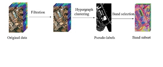
• Designing a noise filtering mechanism based on grid division. By deleting those noise bands, this method can ensure the accuracy of generated pseudo-labels.
• Proposing a hypergraph evolutionary clustering to generate pseudo-labels. By replacing traditional pixels by the centers of super-pixels, this technology significantly reduces the computational cost of generating pseudo-labels, and the designed multi-population ABC obviously improves the quality of clustering.
• Developing a supervised band selection algorithm based on artificial bee colony optimization, which significantly improves the classification accuracy of selected bands.

The remainder of this paper is structured as follows: Section 2 introduces related work including super-pixel segmentation, hypergraph clustering, and artificial bee colony; Section 3 presents the proposed pseudo-label generation method and the supervised band selection algorithm based on ABC; subsequently, Section 4 verifies the effectiveness of the proposed method by experiments; the conclusion is presented in Section 5.

2. Related Work

2.1. Super-Pixel Segmentation

Super-pixel segmentation is proposed and developed in 2003. It refers to irregular pixel blocks with certain visual significance, which are composed of adjacent pixels with similar texture and color characteristics. This technology clusters pixels by using the similarity between them, and replaces a large number of pixels by a small number of super-pixels to express image features. Commonly used super-pixel segmentation algorithms include Graph-based method (Graph-based) [28], fast segmentation algorithm based on geometric flow (Turbo Pixels) [29], simple linear iterative clustering (SLIC) [30], etc.

Compared with other algorithms, SLIC has the advantages of good compatibility for gray-scale images, fast running speed, and compact super-pixels. It first transforms each pixel in the image into Lab space, then combines the three feature components (l, a, b) and the space coordinates (m, n) of Lab space into a five-dimensional vector (l, a, b, m, n). Subsequently, a specified number of initial cluster centers are randomly generated within the five-dimensional vector space, and all pixels are clustered by K-means-like methods. All pixels in the same cluster constitute to a super-pixel. During the execution of SLIC, the distance from a pixel to the cluster center consists of two parts: the pixel distance (D_c) and the spatial distance (D_s):

$$D=D_c+\lambda D_s,\lambda \in [0,1]$$

(1)

where, the parameter $\lambda$ is the distance weight. The larger the $\lambda$ value, the larger the proportion of spatial distance, and the closer those pixels in the same super-pixel.

2.2. Hypergraph Clustering

The concept of hypergraph was first proposed by Claude Berg [31]. Compared with traditional graphs, hypergraphs can better reflect the complexity of spatial relationships between data. At present, hypergraph theory has been used in biology [32,33], image processing [34], pattern recognition [35,36], and so on.

A hypergraph is composed of vertices and hyperedges. Suppose the vertex set is a finite set $V=\{v_1,v_2,\cdots ,v_n\}$, and $E=\{v_1^{\prime },v_2^{\prime },\cdots ,v_m^{\prime }\}$ is a subset cluster of V(or hypergraph), the hypergraph can be expressed as $G=(V,E)$. Figure 1 shows an example with 8 vertices and 3 hypergraphs. Here, two ellipses and one line segment are hyperedges used to divide vertices. These hyperedges constitute three hypergraphs, namely, $E_1=\{v_1,v_2,v_3,v_5\}$, $E_2=\{v_3,v_5,v_6,v_8\}$, and $E_3=\{v_4,v_7\}$.

In addition to the above graphic representation, hypergraph can be represented by an incidence matrix. For a hypergraph containing n vertices and m hyperedges, the incidence matrix is an $m\times n$ matrix. Here, the rows correspond to the vertices of hypergraph, and the columns correspond to the hyperedges of hypergraph. The value of each element in the incidence matrix, $A=\left(a_{ij}\right)$, is:

$$a_{ij}=\left\{\begin{array}{c}1,if{v}_i\in E_j\hfill \\ 0,otherwise\hfill \end{array}\right.$$

(2)

Hypergraph clustering is similar to traditional graph clustering. Its basic idea is to divide the hypergraph repeatedly for reducing the correlation between subgraphs and improving the similarity between vertices within the same subgraph. Figure 2 shows the result of clustering the hypergraph in Figure 1, where the solid line is the result of the redivision, and the dotted line is the result of the original division. It can be seen that after redivision, the similarity between vertices in each subgraph becomes higher.

2.3. Artificial Bee Colony

ABC was proposed by Karaboga [37] by imitating the foraging behavior of bees. Compared with traditional evolutionary optimization techniques such as genetic algorithm, it has the advantages of fast convergence and easy implementation [38].

In ABC, a food source is abstracted as a solution of the optimized problem, and bees searching for food sources are divided into three parts: employed bees, onlooker bees, and scout bees. Employed bees search in the neighborhood of each food source. When a good food source is found, the food source will be used to replace the old one. When all employed bees have completed the search, they fly back to the hive, and some unemployed bees in the hive will turn into onlooker bees. Each onlooker bee selects a good food source with a certain probability, and searches in its neighborhood. If a food source has not been updated for a long time, its position will be initialized by a scout bee.

(1) Employed bee phase: The updated formula of employed bees is as follows:

$$C{x}_{i,d}=x_{i,d}+\phi (x_{i,d}-x_{j,d})$$

(3)

where, i is the index value of the i-th food source, $j(j\ne i)$ is the index value of a food source selected randomly; d is the d-th decision variable, $\phi$ is a random number within [−1, 1], and $C{x}_{i,d}$ is the new position generated by the i-th employed bee.

(2) Onlooker bee phase: Each onlooker bee selects a good food source to search its neighborhood. Taking the i-th food source as an example, the probability that it is selected is:

$$P{r}_i=\frac{fi{t}_i}{{\sum }_{j=1}^{N}fi{t}_j}$$

(4)

$$fi{t}_i=\left\{\begin{array}{c}\frac{1}{f\left(x_i\right)+1},f\left(x_i\right)\ge 0\hfill \\ 1+\left|f\left(x_i\right)\right|,f\left(x_i\right)<0\hfill \end{array}\right.$$

(5)

where, $f\left(\right)$ is the objective function, and N is the number of food sources. After selecting a food source by formula (4), an onlooker bee will search its neighborhood by using formula (3).

(3) Scout bee phase: If the fitness value of a food source has not been improved for $limit$ iterations, it will be reinitialized as follows:

$$x_{new,d}=x_{min,d}+rand(0,1)(x_{max,d}-x_{min,d})$$

(6)

where, $x_{max,d}$ and $x_{min,d}$ are the upper and lower bounds of the d-th decision variable.

3. The Proposed Band Selection Algorithm

3.1. Framework of The Algorithm

In this paper, an unsupervised band selection problem is first transformed into a supervised band selection one by generating pseudo-labels. Figure 3 shows the framework of the proposed algorithm. Firstly, for the input original hyperspectral data, the noise filtering strategy based on grid division is used to delete irrelevant/noise bands. Secondly, the hypergraph evolutionary clustering method with less computational cost is introduced to classify similar pixels into the same category, and label all pixels. On the basis of these pseudo labels, the classification accuracy of a band subset can be calculated. Taking the classification accuracy as the objective function or performance indicator, finally, an evolutionary algorithm is used to optimize the function to find optimal band subset.

3.2. Noise Band Filtering Strategy Based on Grid Division

When labeling hyperspectral data, irrelevant or noise bands in the data seriously affect the accuracy of pseudo-labels. Figure 4 shows the grayscale images of the 120-th and 200-th bands in the data, Indian pines. It can be seen that the image in the 120-th band is clearer, while the noise of the 200-th band is serious. When labeling pseudo-labels, it is clear that the 200-th band will mislead labeling information. In view of this, this paper proposes grid division-based strategy to filter noise bands.

In the proposed filtering strategy, firstly, the hyperspectral image is divided into $n\times n$ grids, and each grid is regarded as a sub-image. Following that, the value of sharpness $Cd$ of each band is calculated:

$$\begin{array}{c}Cd\left(x_i\right)={\displaystyle \sum _{a=1}^{n\times n}}{\displaystyle \sum _{b=1,b\ne a}^{n\times n}}{A}_{tra}^{}(a,b)\hfill \\ s.t.A_{tra}^{}(a,b)=mean\left(\right|x_i^{a\_row}-x_i^{b\_row}\left|\right)+mean\left(\right|x_i^{a\_col}-x_i^{b\_col}\left|\right)\hfill \end{array}$$

(7)

where, $x_i$ represents the i-th band, $x_i^{a\_row}$ and $x_i^{a\_col}$ represent the row vector and the column vector of gray values of the a-th sub-image after dividing the i-th band, respectively; $mean$ is used to get the average of selected vector; $A_{tra}(a,b)$ reflects the difference in grayscale between the sub-images a and b. Finally, according to the value of $Cd$, sort all the bands, and delete the last 10% of bands with lower sharpness.

Generally, the larger the value of $Cd$ of a band, the clearer the land-cover types represented by it. Taking Indian pines in Figure 4 as example, Figure 5 shows the grayscale images of the two bands after dividing $10\times 10$ grids. It can be seen that the grayscale difference between the sub-images in the 112-th band is clearer after division. Furthermore, we select a band in every 60 bands after ranking all bands, Figure 6 shows the grayscale image of theses selected bands for the data, Indian pines. We can see that as the values of $Cd$ decreases, the sharpness of the gray image decreases gradually.

3.3. Pseudo-Label Generation with Hypergraph Evolutionary Clustering

Hypergraph clustering shows good performance in processing data with high-space complexity [39]. However, affected by the quality of initial hypergraph and the weight update method, traditional methods may divide the two vertices belonging to the same class but far apart into two classes. In view of this, this paper studies a hypergraph evolutionary clustering method to label pseudo-labels. Firstly, in order to reduce the computational cost of the clustering algorithm, a super-pixel segmentation method is introduced to select representative pixels. Then, taking these representative pixels as the vertices of the hypergraph, a multi-population ABC with global search capability is proposed to find the optimal combination of hyperedge, and then complete the clustering to hyperspectral pixels. Finally, based on the clustering results, the category of each pixel is labeled.

3.3.1. Super-Pixel Segmentation

Hyperspectral images contain a large number of pixels. If all pixels are used as hypergraph vertices, it will greatly increase the computational cost of the algorithm. In view of this, this paper uses the super-pixel segmentation method to select representative pixels to participate in the subsequent clustering method.

Generally, the SLIC algorithm needs to convert the RGB space of the original image into the Lab space. It has to use three band images to represent the image in the RGB space [30]. However, the number of bands in the hyperspectral image is far more than that of ordinary images. Therefore, three representative bands need to be selected from a large number of bands to generate Lab space images. For more accurate segmentation, the selected representative bands should describe the land-cover types of hyperspectral data to the greatest extent, so we choose the three most informative bands as representatives. The specific method is as follows:

Firstly, calculate the information entropy of all bands, and select the three bands with the largest information entropy to form the Lab image for super-pixel segmentation. Specifically, the information entropy of the i-th band is calculated as follows:

$$\begin{array}{c}H\left(x_i\right)=-\sum p\left(x_i\right)logp\left(x_i\right)\hfill \\ s.t.p\left(x_i\right)=\frac{h\left(x_i\right)}{num}\hfill \end{array}$$

(8)

where, $H\left(x_i\right)$ is the grayscale histogram of the i-th band, and $num$ is the total number of pixels in the band.

Following that, the Lab image is segmented using SLIC super-pixel segmentation method. Taking the data “Pavia University” as example, the segmented image is shown in Figure 7. It can be seen that after super-pixel segmentation, the number of super-pixel blocks is significantly smaller than that of original pixels. The super-pixel segmentation is mapped to all the band, and the center of each super-pixel block is selected as its representative pixel. The hypergraph clustering obviously reduces the number of pixels used, thereby significantly reduce the calculation cost.

3.3.2. ABC-Based Hypergraph Evolutionary Clustering

This section proposes a new hypergraph evolutionary clustering method. This method uses multiple populations to collaboratively search for multiple hypergraphs, where one population is responsible to search for one hypergraph. The hypergraph information is obtained through interaction between these populations. The purpose of interaction is to reduce the number of common vertices and isolated vertices, and guide different populations to search for different hypergraphs. Firstly, the encoding strategy and the optimization index used in the clustering method are given.

(1) Encoding strategy and optimization index

This paper uses a multi-population ABC algorithm to optimize hypergraphs, where the number of populations (N) is equal to or bigger than the number of hypergraphs to be optimized. The dimension of each individual or food source in all populations is equal to the number of vertices, and the binary encoding is used to describe the position of each food source, where “0” means that the current vertex is not selected, and “1” means that it is selected.

Hypergraph clustering usually uses an affinity matrix to calculate the weights of hyperedges. Common indicators used to describe the affinity of data include Euclidean distance, cosine distance, etc. However, it is difficult for these indicators to accurately judge the similarity between data when dealing with high-dimension data. Focused on this, the reference [40] gives a correlation index to measure the similarity between selected bands. Considering the i-th and j-th vertices, $a_i$ and $a_j$, in the hypergraph, their affinity value is as follows:

$$R(a_i,a_j)=\frac{mean(a_i·a_j)-mean\left(a_i\right)\times mean\left(a_j\right)}{\sqrt{mean(a_i·a_i)-mea{n}^2\left(a_i\right)}\sqrt{mean(a_j·a_j)-mea{n}^2\left(a_j\right)}}$$

(9)

where, $a·b$ represents the dot product between a and b.

For a hypergraph containing l vertices, the affinity values between all vertices are calculated in turn. On the basis of their mean value, the hyperedge weight of the hypergraph (w) can be determined. Since the hypergraph clustering method needs to maximize the weight of the hyperedge of each hypergraph, the weight of the hyperedge of the k-th hypergraph is used as the objective function, which is optimized by the k-th population:

$$max{f}_k=w_k=\frac{1}{l(l-1)}\sum _{i=1}^l\sum _{j=1}^{l}R(a_i,a_j)$$

(10)

(2) Multi-population coordination strategy

In the proposed algorithm, one population is only used to search one hypergraph. To prevent multiple populations from searching for the same hypergraph, this section proposes a multi-population coordination strategy to remove common vertices and isolated vertices. After each iteration of ABC, each population selects the optimal solution obtained so far, noted by $p_{i,best},i=1,2,\cdots ,N$. This optimal solution is the optimal hypergraph obtained by the population so far. Based on this, the N populations can get N hypergraphs. Then, common vertices and isolated vertices are identified from all N hypergraphs, and are re-assigned to a unique hypergraph. The specific strategy is as follows:

Case 1: Isolated vertices

An isolated vertex is the one not included in any existing hypergraphs. The strategy of dealing with an isolated vertex is as follows: firstly, calculate the hyperedge weight of each existing hypergraph, and record the hyperedge weight of the i-th hyper graph as $w_i\left(0\right)$. Secondly, allocate the isolated vertex to all hypergraphs respectively, and re-calculate their hyperedge weights. The new hyperedge weight of the i-th hypergraph is recorded as $w_i\left(1\right)$. Then, compare the difference, $\mathsf{\Delta }{w}_i=w_i\left(1\right)-w_i\left(0\right),i=1,2,...,N$, and determine the hypergraph with the maximum difference, note the maximum difference by $\mathsf{\Delta }{w}_{max}$. When $\mathsf{\Delta }{w}_{max}^{}>0$, allocate the isolated vertex into the hypergraph with the largest difference.

Taking the case of 4 populations as the example, Figure 8 illustrates the process of dealing with isolated vertices. Figure 8a shows the hypergraph obtained by the 4 populations after iterations, namely, $p_{i,best},i=1,2,3,4$. We can see that the second and fourth vertices are not selected by any hypergraph (their corresponding values are all 0), so they are isolated vertices. Supposing that the hyperedge weight of $p_{2,best}$ achieves the most improvement when adding the isolated vertex $v_2$, then $v_2$ is only inserted into $p_{2,best}$, that is, $p_{2,best}\left(v_2\right)=1$. However, the weights of all hyperedges are not improved by adding $v_4$, so we do not do anything about it.

Case 2: Common vertices existing in multiple hypergraphs

A common vertex is the one that appears in multiple hypergraphs at the same time. For each common vertex found, firstly, find all the hypergraphs containing it, and calculate their hyperedge weights, denoted by $w_i^{\prime }\left(0\right),i=1,2,\cdots ,N$. Secondly, remove the common vertex from these hypergraphs, and re-calculate the hyperedge weights of these hypergraphs, denoted by $w_i^{\prime }\left(1\right),i=1,2,\cdots ,N$. Next, calculate the attenuation degree of each hypergraph before and after removing the common vertex, $\mathsf{\Delta }{w}_i^{\prime }=w_i^{\prime }\left(0\right)-w_i^{\prime }\left(1\right),i=1,2,\cdots ,N$; following that, find the hypergraph with the greatest attenuation, denoted by the k-th hypergraph. When $\mathsf{\Delta }{w}_k^{\prime }>0$, put the common vertex back to the k-th hypergraph; Otherwise, it is completely removed from all the hypergraphs, and becomes an isolated vertex.

Figure 9a shows the hypergraphs obtained by the 4 populations. It can be seen that the vertex $v_1$ is selected by three hypergraphs at the same time, the vertex $v_3$ is selected by two hypergraphs at the same time, so they are common vertices. Supposing that the hyperedge weight of $p_{1,best}$ gets the maximum attenuation after the vertex $v_1$ is deleted, the vertex remains in $p_{1,best}$, but is deleted from $p_{2,best}$ and $p_{4,best}$. After deleting the vertex $v_3$ from $p_{3,best}$ and $p_{4,best}$, their hyperedge weights all become better; that is, their attenuation values are all less than 0. Therefore, the vertex $v_3$ needs to be completely deleted from the two hypergraphs, and becomes an isolated vertex.

After the above operations, if the optimal hypergraph of a population ($p_{i,best}$) is updated, and the hyperedge weight of the updated hypergraph ($p_{i,best}^{\prime }$) becomes big, $p_{i,best}^{\prime }$ will be used to replace the worst food source in the population; otherwise, delete $p_{i,best}^{\prime }$.

(3) Steps of the proposed hypergraph evolutionary clustering algorithm

Based on the above work, Algorithm 1 gives the detailed steps of the proposed hypergraph evolutionary clustering based on ABC. Firstly, initialize the parameters of SLIC, and normalize the data to 0–255 (Line 1); secondly, use the method proposed in Section 3.2 to remove noise and irrelevant bands (Line 2); next, use the super-pixel segmentation technology to divide the image into multiple super-pixel blocks, and select the center of each super-pixel block as its representative (Line 3); then, using selected super-pixel centers as the super-vertices, and the proposed multi-population ABC is implemented to search the N optimal hypergraphs (Lines 6–13). Here, $iter0$ represents the current iterations, and $ma{x}_{i}ter0$ represents the maximum iterations of the algorithm.

Furthermore, inspired by the idea of particle swarm optimization, an optimal solution guided update strategy is proposed to improve the search speed of employed bee:

$$p_{i,new}=p_{i,best}+{\phi }_1(p_{i,r1}-p_{i,r2})$$

(11)

where, $p_{i,new}$ is the position of a food source in the i-th population, $p_{i,best}$ is the optimal food source in the population, $p_{i,r1}$ and $p_{i,r2}$ are two random food sources in the i-th population, $r1\ne r2$. In the phases of onlooker bees and scout bees, traditional methods are still used to update the positions of food sources.

Algorithm 1: The proposed hypergraph evolutionary clustering based on ABC, HC-ABC.

Input: Hyperspectral image data, X;

Output: Optimal solution set, $\left\{p_{i,best}\right|i=1,2,\cdots ,N\}$;

1. Initialize the parameters of SLIC, and normalize the X to 0–255;

2. Filter out irrelevant or noise bands by the method in Section 3.2;

3. Execute the method in Section 3.3.1 to get the super-pixel centers;

4. Initialize the parameters of ABC, and randomly initialize the N populations;

5. While ($iter0<ma{x}_{iter0}$)

6.   For $i=1:N$      % Simultaneously update the food sources in the N populations.

7.     Calculate the fitness value of each food source in the population by formula (10),

and find the optimal solution, $p_{i,best}$;

8.      Employed bee phase: Update all the food sources by formula (11);

9.      Onlooker bee phase: Update the selected food sources by formula (3);

10.     Scout bee phase: Reinitialize the stagnant food sources by formula (6);

11.   End for

12.    Execute the multi-population coordination strategy, update the $p_{i,best}$ of each population;

13.    $iter0=iter0+1$;

14. End while

15. Output the $p_{i,best},i=1,2,\cdots ,N$ obtained by every population.

3.3.3. Generation of The Pseudo-Labels

By Algorithm 1, all super-pixel vertices can be divided into h optimal hypergraphs. Here, a hypergraph is recorded as one category, so we can obtain h categories. Since each vertex used $in$ hypergraph clustering is the pixel center of a super-pixel, all pixels in the same super-pixel have the same class label with its pixel center.

3.4. ABC-Based Supervised Band Selection Algorithm

After generating pseudo-labels using Section 3.3, an unsupervised band selection problem is transformed into a supervised one. According to the generated pseudo-labels, this paper takes the classification accuracy of band subset as the objective function to be optimized, and ABC is used to find the optimal band subset. The expression of the objective function is as follows:

$$maxF=OA\left(V\right)+AA\left(V\right)$$

(12)

where, V is a band subset, $OA$ represents the ratio of correct classification pixels to all pixels under the current band subset, $AA$ represents the average of the ratio of correct classification pixels in each category under the current band subset. Now scholars have proposed many typical classifiers, such as SVM, KNN, Bayes, etc. Since this paper focuses mainly on the process of band selection, without loss of generality, this paper uses the most commonly used KNN to predict the category of a pixel.

When using ABC to optimize the problem (12), the binary encoding is used to represent the position of food source. A food source corresponds to a subset of bands. For the j-th element of a food source, “1” means the j-th band is selected; otherwise, not selected. The employed bees use the formula (11) to update the position of food source, and the onlooker bees and scout bees still use the formulas in Algorithm 1. The final optimal food source obtained by ABC is the best band subset, $Best$.

After obtaining $Best$, furthermore, this paper uses the max-relevance and min-redundancy (mRMR) to generate a band subset of specified size from $Best$:

$$mRMR=\underset{b_j\in Best/S_{m-1}}{max}\left[I(b_j;Y)-\frac{1}{m-1}\sum _{b_i\in S_{m-1}}I(b_j;b_i)\right]$$

(13)

where, $I(b_j;Y)$ represents the mutual information between the band $b_j$ and the pseudo-labels Y, $I(b_j;b_i)$ represents the mutual information between the bands $b_j$ and $b_j$; $S_{m-1}$ represents the set of selected bands, and $B/S_{m-1}$ represents the set of unselected bands.

In order to express the proposed band selection algorithm clearly, its detailed implement steps are described as follows:

Step1: Input and normalize the hyperspectral data to be processed; initialize related parameters including the population size, the maximum number of iterations, the number of super-pixel blocks, the proportion of spatial distance, the threshold of segmentation image gradient, and so on.

Step2: Implement the noise band filtering strategy based on grid division in Section 3.2 to delete those noise bands.

Step3: Generate pseudo-labels for all the remaining bands by using the proposed hypergraph evolutionary clustering method in Section 3.3.

Setp4: Implement the supervised band selection algorithm based on ABC to find the optimal band subsets, as follows:

Step4.1: Initialization. Randomly generate the positions of $FN$ food sources within the search space. This paper uses the binary encoding to represent the position of a food source. Taking a food source as example, its expression is as follows.

$$X=(x_1,x_2,...,x_D),x_i\in \{0,1\}$$

(14)

where $x_i=1$ indicates the $i-th$ band is selected into the band subset; otherwise, it is not.

Step4.2: Calculate the fitness value of each food source by formula (12), and determine the best optimal solution $p_{best}$ from the current population.

Step4.3: Employed bee phase: Use formula (11) to update employed bees; calculate the fitness values of each new position by formula (12). If the new position of an employed bee is superior to its corresponding food source, the food source is replaced by the new position.

Step4.4: Onlooker bee phase: Calculate the follow probability of each food source; select a food source for each onlooker bee according to these probability values, then update the positions of onlooker bees according to formula (3). Next, calculate the fitness values of each new position by formula (12). If the new position of an onlooker bee is superior to its corresponding food source, the food source is replaced by the new position.

Step4.5: Scout bee phase: If a food source cannot be improved after the $Limit$ iterations, its associated onlooker bee becomes a scout bee. The position of scout bee is randomly initialized.

Step4.6: Determine the best optimal solution $p_{best}$ from the current population.

Step4.7: Whether the maximum iteration time is satisfied. If yes, stop and output $p_{best}$; otherwise, return to Step 4.3.

3.5. Algorithm Complexity

The computational complexity of the proposed HC-ABC algorithm mainly consists of three phases, i.e., the super-pixel segmentation, the hypergraph evolutionary clustering, and the band selection based on ABC.

In the phase of super-pixel segmentation, the clustering algorithm runs the basic operator $O(Iter\times NL\times S)$ times, where $NL$ is the number of super-pixel blocks, $Iter$ is the iteration times, and S is the neighborhood scale of each class of SLIC.

In the phase of hypergraph evolutionary clustering, the calculation complexity mainly focuses on the evaluation of candidate solutions. Here, the complexity of evaluating a single solution is $O\left(N{L}^2\right)$. Therefore, the complexity of this operator is $O(3C\times NC\times D^2)$, where C is the number of land-cover types in a dataset, $NC$ is the number of candidate solutions to be evaluated.

In the phase of band selection, the calculation cost mainly focuses on implementing the classifier. We evaluate each individual through the classifier KNN in this paper. The complexity of KNN is $O(D\times Tr\times Ts)$, where, D is the dimension of data, $Tr$ is the number of training samples, and $Ts$ is the number of test samples. Therefore, the computational complexity of this phase is $O(NP\times D\times Tr\times Ts)$, where $NP$ is the population size.

For hyperspectral image data, $Tr$ and $Ts$ are much larger than other parameters. Therefore, the computational complexity of HC-ABC is $O(NP\times D\times Tr\times Ts)$.

4. Experiment and Analysis

This section analyzes the effectiveness of the proposed HC-ABC algorithm through experiments.

4.1. Experiment Preparation

The experiments are divided into two parts. The first part is to verify the effectiveness of the proposed hypergraph evolutionary clustering method by comparing it with two typical clustering algorithms. In the second part, the proposed HC-ABC algorithm is compared with six existing band selection algorithms to verify its effectiveness. The selected comparison algorithms include two cluster-based algorithms (Waludi [41] and SNNCA [42]), two rank-based algorithms (ER [43] and MVPCA [44]), and two evolutionary optimization-based algorithms (MI-DGSA [45] and ISD-ABC [46]).

Waludi uses a layer-by-layer clustering strategy to group bands, and uses the divergence as a criterion to measure the correlation between bands. SNNCA introduces a clustering strategy based on Shared Near Neighbors, and combines the information entropy and correlation to select representative bands from clustering results. ER calculates the information entropy of each band, and selects a number of bands with the largest information entropy to form the band subset. MVPCA estimates the priority of each band through the load factor, and sorts all the bands according to the priority. MI-DGSA uses Maximum Information and Minimum Redundancy (MIMR) as an indicator to search for optimal band subset by a discrete gravitational search algorithm. ISD-ABC is an artificial bee colony algorithm based on subspace decomposition.

Three important indexes are used to evaluate the performance of an algorithm. They are overall accuracy (OA), average accuracy (AA), and Kappa coefficient (KC). Formula (12) shows the definitions of OA and AA, where OA can describe the global classification performance of an algorithm, while AA can reflect the classification performance of each category. KC is used to describe the consistency between the classification result obtained by an algorithm and the real categories.

In order to reduce the evaluation bias of classifier on the performance of algorithm, three widely used classifiers are selected, i.e., Random Forest (RAF), SVM, and KNN. In Random Forest, the number of trees is set to be 50, and other parameters are set to be their default values. In SVM, we use a pair of all-in-one methods to deal with the multi-classification problem, and chose the radial basis as the kernel function, whose corresponding parameters are determined by the 50% cross validation method. In KNN, the number of nearest neighbors is set to be 3. In all experiments, 20% samples of each category are randomly selected as training samples, and the remaining samples are used as test samples.

4.2. Data Description

The first dataset is Indian Pines. The dataset contains 220 bands, with wavelengths ranging from 400 to 2500 nanometers, and each band image is made up of 145 pixels. The dataset contains 16 types of land-cover, and the grayscale image is shown in Figure 10. The white part in the figure is the land-cover type that has been marked.

The second dataset is Pavia University, belonging to the urban environment. The dataset is composed of 115 bands, each band image is made up of 610 pixels. It includes 9 land-cover types, and the grayscale image is shown in Figure 11. The white part in the figure is the land-cover type that has been marked.

The third dataset is Salinas, captured from the sky above Salinas Valley. It is made up of 224 bands, each band image is made up of 512 pixels. It includes 16 land-cover types, and the grayscale image is shown in Figure 12. The white part in the figure is the land-cover type that has been marked.

4.3. Analysis of Parameters

The proposed algorithm includes three parts, i.e., the super-pixel segmentation, the hypergraph evolutionary clustering, and the band selection.

In phase of super-pixel segmentation, there are three key parameters in SLIC, i.e., the number of super-pixel blocks, the proportion of spatial distance, and the threshold of segmentation image gradient $\theta$. We set different values for the three parameters, and run the proposed band selection algorithm on the Indian Pines dataset. According to the results of classification experiment, we found that the proposed algorithm is less sensitive to the spatial distance proportion. Therefore, this paper still uses the value suggested in [47].

For the other two parameters, Figure 13 and Figure 14 show the classification accuracy curves obtained by the proposed algorithm with different parameter values. From Figure 13, we can see that the classification accuracy gradually improves when the number of super-pixel blocks increases from 50 to 100. However, when the number of super-pixel blocks is greater than 100, the rising speed of the OA value decreases significantly. On the other hand, the running time of the algorithm will increase as the number of super-pixel blocks increases. In order to compromise the above two points, we set the number of super pixel blocks to 100 in the experiments.

From Figure 14, we can see that the OA value obtained by the algorithm is the largest when the segmentation image gradient threshold $\theta =0.01$. This conclusion is the same as the recommended value in [47]. Therefore, we still use the value of $\theta =0.01$.

The key parameters used in the other two parts include the size of population used by evolutionary clustering, $NC$, and the size of population used by band selection, $NP$.

Table 1. The OA values obtained by the proposed algorithm with different $NC$ values.

Number of $\mathit{NC}$	5	10	15	20	25	30	35	40
OA %	73.374	74.465	75.132	75.653	75.680	75.665	75.700	75.662

and

Table 2. The OA values obtained by the proposed algorithm with different $NP$ values.

Number of $\mathit{NP}$	10	20	30	40	b	60	70	80
OA %	72.992	73.742	74.563	75.3463	75.678	75.669	75.672	75.681

show the classification accuracy curves obtained by the proposed algorithm with different $NC$ and $NP$ values, respectively. From Table 1, we can see that the OA value of the proposed algorithm increases as the population size $NC$ increases. When the value of $NC$ is greater than 20, the OA value has no obvious change. Therefore, we set $NC=20$ in the proposed algorithm. From Table 2, we can see that similar to $NC$, the evolutionary algorithm can find the global optimal solution when $NP=50$. Therefore, we set $NP=50$ in the proposed algorithm.

In addition, for a fair comparison, the proposed algorithm and the two comparison algorithms (MI-DGSA and ISD-ABC) all set the same maximum iteration times, 200.

4.4. Analysis on the Hypergraph Evolutionary Clustering

In order to verify the effectiveness of the proposed hypergraph evolutionary clustering method, this section selects two different types of clustering algorithms as the comparison method. K-mean is a very representative method in decentralized clustering technologies, and it has a wide range of applications in many fields. The layer-by-layer clustering is the most commonly used one in structural clustering technologies. Due to its strong universality and good clustering performance, we choose it as another comparison algorithm. In addition, they are both suitable for processing large-scale data such as hyperspectral data.

For convenience, the HC-ABC using K-mean clustering called K-mean-ABC, and the HC-ABC using layer-by-layer clustering called LBL-ABC. Figure 15, Figure 16 and Figure 17 show the OA values of band subsets obtained by the three algorithms with the three classifiers.

For the Indian Pines, it can be seen from Figure 15 that the results of HC-ABC all are significantly better than that of LBL-ABC and K-mean-ABC under the three classifiers. Specifically: (1) For the classifiers KNN and SVM, when the number of selected bands is less than 11, the OA value of HC-ABC is about 5% higher than that of LBL-ABC and K-mean-ABC. With the increase of the number of selected bands, the difference in the OA value between HC-ABC and the two comparison algorithms gradually decreases, but HC-ABC is still about 2% higher than the two comparison algorithms. (2) For the classifier RAF, when the number of selected bands is less than 9, the OA value of HC-ABC is significantly higher than that of LBL-ABC and K-mean-ABC; with the increase of the number of selected bands, the difference in the OA value between HC-ABC and LBL-ABC decreases. The OA value of HC-ABC is still about 2% higher than that of K-mean-ABC. (3) Considering the three classifiers comprehensively, the fluctuation degree of the OA values obtained by HC-ABC is significantly smaller than that of LBL-ABC and K-mean-ABC, as the number of selected bands increases.

For the Pavia University, it can be seen from Figure 16 that: (1) When the number of selected bands is low, the OA value of HC-ABC is slightly smaller than that of LBL-ABC; however, when the number of selected bands is greater than 30, the OA values of HC-ABC on the three classifiers are about 4% higher than those of LBL-ABC and K-mean-ABC. In addition, when the number of selected bands is between $[7,30]$, for the classifiers KNN and SVM, the OA values of HC-ABC are about 1% higher than that of LBL-ABC, and about 2% higher than that of K-mean-ABC; for the classifier RAF, HC-ABC, and LBL-ABC get similar OA values, and their values are about 2% higher than that of K-mean-ABC.

For the Salinas, it can be seen from Figure 17 that for the three classifiers, the OA values of HC-ABC all are significantly higher than that of LBL-ABC and K-mean-ABC. Specifically: (1) When the classifiers KNN and RAF are used, the OA values of HC-ABC are about 2% higher than that of K-men-ABC and about 4% higher than that of LBL-ABC. (2) When using the classifier SVM, the OA value of HC-ABC is higher than that of K-mean-ABC. When the number of selected bands is greater than 30, the OA value of LBL-ABC has been greatly improved; in particular, when the numbers of selected bands are 34 and 35, the OA values of LBL-ABC are slightly higher than that of HC-ABC.

Overall, compared with the two existing clustering methods, the proposed hypergraph clustering can help the proposed band selection algorithm to obtain better results, so it is an effective strategy to generate pseudo-label for hyperspectral images.

4.5. Comparison Results

4.5.1. Comparison on the Classification Performance

This experiment compares HC-ABC with 6 existing band selection algorithms, i.e., Waludi, SNNCA, ER, MVPCA, ISD-ABC, and MI-DGSA. Figure 18, Figure 19 and Figure 20 show the average OA and AA values obtained by the seven algorithms. For fairness, the number of bands when all the algorithms are relatively stable is used to calculate their AA values. Specifically, the number of bands is set to be 30 in this paper.

For the Indian Pines, it can be seen from Figure 18 that HC-ABC achieved better OA and AA values when using 3 classifiers. Specifically: (1) For the classifier KNN, when the number of selected bands is between 3–9, the OA values of HC-ABC are slightly lower than that SNNCA, but significantly higher than that of the other 5 comparison algorithms; with the increase of the number of selected bands, the OA values of HC-ABC are significantly higher than that of all the comparison algorithms. (2) For the classifiers RAF and SVM, HC-ABC, and SNNCA have similar OA values, which are significantly better than the other 5 comparison algorithms; when the number of selected bands is 17–30, the OA values of HC-ABC are significantly better than that of SNNCA. (3) When using the classifiers KNN and RAF, the AA values of HC-ABC are significantly higher than that of the six comparison algorithms; when using the classifier SVM, HC-ABC and Waludi achieved similar AA values. Th reason may be that the band subset of 30 bands is not the best result of HC-ABC.

For the Pavia University, it can be seen from Figure 19 that the OA values of HC-ABC show the same trend when the three classifiers are used, which is better than the six comparison algorithms in most cases. Specifically: (1) When using the KNN classifier, the OA value of HC-ABC is significantly better than that of the 6 comparison algorithms, except for part special number of bands. (2) For the classifier RAF, when the number of selected bands is less than 6, the OA values of HC-ABC are slightly lower than that of SNNCA and MVPCA, but still higher than that of the other four comparison algorithms; when the number of selected bands is greater than 6, the OA values of HC-ABC have been significantly improved compared with other comparison algorithms. (3) When using the classifier SVM, the OA value of HC-ABC is slightly lower than that of SNNCA or MVPCA for part special numbers of band; however, for other cases, the results of HC-ABC are better than that of all the 6 comparison algorithms. (4) In addition, the AA values of HC-ABC on the three classifiers are higher than that of all the 6 comparison algorithms.

For the Salinas, it can be seen from Figure 20: (1) In most cases, the OA values of HC-ABC are significantly higher than that of the other comparison algorithms. Specifically, when the number of selected bands is small, the OA values of HC-ABC are lower than that of SNNCA or MVPCA; however, with the increase of the number of bands, the OA values of HC-ABC are significantly better than that of the other 6 comparison algorithms. (2) When using the classifiers KNN and RAF, the AA values of HC-ABC are significantly higher than that of the other 6 comparison algorithms. When using the classifier SVM, the AA values of HC-ABC and Waludi are very close, but their OA values are significantly better than that of Waludi. The possible reason is that the band subset selected by HC-ABC has a high classification accuracy for land-cover types with more samples, but has a low classification accuracy for land-cover types with small samples.

In order to compare the classification performance of each algorithm better,

Table 3. The average performance values of the 7 algorithms on all the three data sets.

Data	Algorithms	KNN			RAF			SVM
		OA	AA	KC	OA	AA	KC	OA	AA	KC
Indian Pines	Waludi	0.6769	0.6323	0.6297	0.7057	0.6078	0.6624	0.7448	0.6852	0.7052
		±0.0596	±0.0679	±0.0684	±0.0455	±0.0402	±0.0524	±0.0754	±0.1102	±0.0919
	ER	0.6324	0.5609	0.5792	0.6449	0.5469	0.5907	0.6584	0.5639	0.5996
		±0.0665	±0.0678	±0.0761	±0.0668	±0.0743	±0.0773	±0.1039	±0.1415	±0.1280
	MI-DGSA	0.6375	0.5875	0.5851	0.6748	0.6119	0.6257	0.7231	0.6710	0.6798
		±0.0273	±0.0283	±0.0313	±0.0303	±0.0337	±0.0349	±0.0583	±0.0908	±0.0717
	ISD-ABC	0.6215	0.5657	0.5666	0.6563	0.5855	0.6041	0.7069	0.6432	0.6607
		±0.0247	±0.0242	±0.0284	±0.0287	±0.0303	±0.0340	±0.0556	±0.0837	±0.0691
	MVPCA	0.6916	0.6415	0.6467	0.7098	0.6133	0.6707	0.7564	0.7011	0.7196
		±0.0500	±0.0512	±0.0577	±0.0436	±0.0368	±0.0501	±0.0672	±0.1021	±0.0808
	SNNCA	0.7084	0.6394	0.6669	0.7198	0.6232	0.6809	0.7680	0.7114	0.7340
		±0.0313	±0.0323	±0.0359	±0.0310	±0.0262	±0.0354	±0.0564	±0.0843	±0.0676
	HC-ABC	0.7302	0.6520	0.6908	0.7275	0.6300	0.6854	0.7807	0.7295	0.7477
		±0.0402	±0.0344	±0.0260	±0.0294	±0.0195	±0.0337	±0.0521	±0.0785	±0.0617
Pavia university	Waludi	0.8432	0.8130	0.7902	0.8551	0.8215	0.8102	0.8912	0.8617	0.8718
		±0.0232	±0.0256	±0.0314	±0.0259	±0.0283	±0.0353	±0.0434	±0.0646	±0.0618
	ER	0.8029	0.7506	0.7359	0.8075	0.7372	0.7387	0.8403	0.7439	0.7789
		±0.1025	±0.1295	±0.1399	±0.0951	±0.1220	±0.1321	±0.0915	±0.1495	±0.1354
	MI-DGSA	0.8577	0.8276	0.7841	0.8587	0.8189	0.7899	0.8867	0.8394	0.8403
		±0.0194	±0.0245	±0.0262	±0.0208	±0.0256	±0.0284	±0.0232	±0.0446	±0.0339
	ISD-ABC	0.8331	0.8015	0.7577	0.8478	0.8056	0.7767	0.8734	0.8248	0.8256
		±0.0227	±0.0277	±0.0307	±0.0240	±0.0282	±0.0327	±0.0257	±0.0477	±0.0376
	MVPCA	0.8545	0.8273	0.8078	0.8605	0.8254	0.8160	0.8905	0.8551	0.8792
		±0.0352	±0.0425	±0.0474	±0.0364	±0.0442	±0.0493	±0.0530	±0.0822	±0.0754
	SNNCA	0.8515	0.8304	0.8106	0.8670	0.8390	0.8249	0.8998	0.8730	0.8801
		±0.0206	±0.0203	±0.0279	±0.0184	±0.0174	±0.0248	±0.0378	±0.0502	±0.0532
	HC-ABC	0.8700	0.8407	0.8244	0.8863	0.8549	0.8463	0.9056	0.8596	0.8918
		±0.0237	±0.0287	±0.0324	±0.0249	±0.0250	±0.0336	±0.0386	±0.0593	±0.0547
Salinas	Waludi	0.8745	0.9261	0.8802	0.9009	0.9410	0.8896	0.8977	0.9337	0.8855
		±0.0332	±0.0384	±0.0371	±0.0238	±0.0266	±0.0265	±0.0418	±0.0491	±0.0474
	ER	0.8364	0.8671	0.8377	0.8524	0.8747	0.8354	0.8527	0.8714	0.8350
		±0.0434	±0.0596	±0.0487	±0.0400	±0.0550	±0.0448	±0.0429	±0.0739	±0.0489
	MI-DGSA	0.8709	0.9241	0.8762	0.8920	0.9319	0.8797	0.8953	0.9324	0.8830
		±0.0136	±0.0163	±0.0152	±0.0133	±0.0138	±0.0148	±0.0222	±0.0255	±0.0250
	ISD-ABC	0.8658	0.9195	0.8706	0.8840	0.9252	0.8708	0.8930	0.9299	0.8806
		±0.0117	±0.0137	±0.0131	±0.0123	±0.0122	±0.0137	±0.0207	±0.0232	±0.0233
	MVPCA	0.8816	0.9313	0.8893	0.9061	0.9469	0.8954	0.9087	0.9463	0.8980
		±0.0095	±0.0082	±0.0106	±0.0126	±0.0098	±0.0140	±0.0158	±0.0138	±0.0177
	SNNCA	0.8814	0.9302	0.8890	0.9034	0.9450	0.8924	0.9095	0.9461	0.8990
		±0.0166	±0.0153	±0.0185	±0.0163	±0.0137	±0.0182	±0.0230	±0.0234	±0.0259
	HC-ABC	0.8919	0.9442	0.8998	0.9156	0.9602	0.9082	0.9222	0.9549	0.9157
		±0.0176	±0.0126	±0.0188	±0.0193	±0.0165	±0.0180	±0.0227	±0.0157	±0.0221

lists the average and variance of classification accuracy of all band subsets obtained by each algorithm. In addition to the OA and AA indexes, the KC indicator has also been used. It can be seen from Table 3 that HC-ABC obtained the best average classification accuracy on all datasets. Taking Indian Pines as example, when the KNN classifier is used, the average values of HC-ABC on the three indexes are 0.7302, 0.6520, and 0.6908, respectively, while the maximum values obtained by the other six algorithms are 0.7084, 0.6394, and 0.6669, respectively.

4.5.2. Significance Analysis

This section uses a parametric test (i.e., t-test) and a non-parametric test (i.e., Post-hoc) to compare the significant differences between two algorithms. Where, the t-test is a kind of parametric test, and Post-hoc is a non-parametric statistical test. Although they often are used to compare the significant difference between the two sets of solutions which have a normal distribution, many literatures [13,48,49] about evolutionary feature selections still use them to test the performance of algorithms. Therefore, we also use them to compare the significant difference between two algorithms in this paper. For these two statistical tests, the confidence interval of the hypothesis test both is set to 98%.

Table 4. The results of t-test on the seven algorithms.

Classifier	Waludi	ER	MI-DGSA	ISD-ABC	MVPCA	SNNCA	HC-ABC
KNN	+	+	+	+	+	+	\
RAF	+	+	+	+	+	≈	\
SVM	+	+	+	+	+	≈	\

and

Table 5. The results of Post-hoc on the seven algorithms.

Classifier	Waludi	ER	MI-DGSA	ISD-ABC	MVPCA	SNNCA	HC-ABC
KNN	+	+	+	+	+	+	\
RAF	+	+	+	+	≈	+	\
SVM	+	+	+	+	+	-	\

record their test results between HC-ABC and the six comparison algorithms, respectively. Here, ‘+’ means that HC-ABC is significantly better than the comparison algorithm, ‘-’ means that HC-ABC is significantly inferior to the comparison algorithm, and ’≈’ means there is no significant difference between the two.

It can be seen that, in most cases, the results obtained by HC-ABC are significantly better than that of the other six comparison algorithms. When using the classifiers RAF and SVM, the t-test test results show that there is no significant difference between SNNCA and HC-ABC; when using the classifier SVM, the Post-hoc test results show that the performance of SNNCA are significantly better than that of HC-ABC. All these results indicate that the proposed HC-ABC is a highly competitive algorithm to deal with hyperspectral band selection problems.

5. Conclusions

For the problem of unsupervised band selection, this paper studied a pseudo-label guided artificial bee colony algorithm. Both the proposed noise filtering mechanism with grid division and the proposed hypergraph evolutionary clustering method obviously improve the quality of generated pseudo-labels. The introduced ABC-based supervised band selection algorithm significantly improves the classification accuracy of selected bands. The proposed band selection algorithm was compared with 6 existing algorithms (Waludi, SNNCA, ER, MVPCA, MI-DGSA, and ISD-ABC), and experimental results showed that it is superior to these comparison algorithms in term of three classification indicators in most cases.

Since needing to use the classification accuracy to evaluate new solutions repeatedly, the proposed algorithm in this paper has a relatively high computation cost. How to use marching learning technologies to reduce its computation cost is a key issue for our future research. In addition, how to design a more effective supervised band selection algorithm is another key issue to be studied.

MDPI stays neutral with regard to jurisdictional claims in published maps and institutional affiliations.

References

1. Acosta, I.C.C.; Khodadadzadeh, M.; Tusa, L.; Ghamisi, P.; Gloaguen, R. A machine learning framework for drill-core mineral mapping using hyperspectral and high-resolution mineralogical data fusion. IEEE J. Sel. Top. Appl. Earth Obs. Remote Sens. 2019, 12, 4829–4842. [Google Scholar] [CrossRef]
2. Nguyen, H.D.; Nansen, C. Hyperspectral remote sensing to detect leafminer-induced stress in bok-choy and spinach according to fertilizer regime and timing. Pest Manag. Sci. 2020, 76, 2208–2216. [Google Scholar] [CrossRef] [Green Version]
3. Li, Y.; Lu, T.; Li, S.T. Subpixel-pixel-superpixel-based multiview active learning for hyperspectral images classification. IEEE Trans. Geosci. Remote Sens. 2020, 58, 4976–4988. [Google Scholar] [CrossRef]
4. Azar, S.G.; Meshgini, S.; Rezaii, T.Y.; Beheshti, S. Hyperspectral image classification based on sparse modeling of spectral blocks. Neurocomputing 2020, 407, 12–23. [Google Scholar] [CrossRef]
5. Hughes, G. On the mean accuracy of statistical pattern recognizers. IEEE Trans. Inf. Theory 1968, 14, 55–63. [Google Scholar] [CrossRef] [Green Version]
6. Xie, F.; Li, F.; Lei, C.; Ke, L. Representative band selection for hyperspectral image classification. ISPRS Int. J. Geo-Inf. 2018, 7, 338. [Google Scholar] [CrossRef] [Green Version]
7. Pham, D.S.; Ridley, J.; Lazarescu, M. An efficient feature extraction method for the detection of material rings in rotary kilns. IEEE Trans. Ind. Inform. 2020, 16, 5914–5923. [Google Scholar] [CrossRef]
8. Zhang, Y.; Cheng, S.; Gong, D.W.; Shi, Y.H.; Zhao, X.C. Cost-sensitive feature selection using two-archive multi-objective artificial bee colony algorithm. Expert Syst. Appl. 2019, 137, 46–58. [Google Scholar] [CrossRef]
9. Li, M.M.; Wang, H.F.; Yang, L.F.; Liang, Y.; Shang, Z.G.; Wang, H. Fast hybrid dimensionality reduction method for classification based on feature selection and grouped feature extraction. Expert Syst. Appl. 2020. [Google Scholar] [CrossRef]
10. Habermann, M.; Fremont, V.; Shiguemori, E.H. Supervised band selection in hyperspectral images using single-layer neural networks. Int. J. Remote Sens. 2019, 40, 3900–3926. [Google Scholar] [CrossRef]
11. Cao, X.H.; Xiong, T.; Jiao, L.C. Supervised band selection using local spatial information for hyperspectral image. IEEE Geosci. Remote Sens. Lett. 2016, 13, 329–333. [Google Scholar] [CrossRef]
12. Song, X.F.; Zhang, Y.; Guo, Y.N.; Sun, X.Y. Variable-size cooperative coevolutionary particle swarm optimization for feature selection on high-dimensional data. IEEE Trans. Evol. Comput. 2020. [Google Scholar] [CrossRef]
13. Hu, Y.; Zhang, Y.; Gong, D.W. Multi-objective particle swarm optimization for feature selection with fuzzy cost. IEEE Trans. Cybern. 2020. [Google Scholar] [CrossRef] [PubMed]
14. Sui, C.H.; Li, C.; Feng, J.; Mei, X.G. Unsupervised manifold-preserving and weakly redundant band selection method for hyperspectral imagery. IEEE Trans. Geosci. Remote Sens. 2020, 58, 1156–1170. [Google Scholar] [CrossRef]
15. Bevilacqua, M.; Berthoumieu, Y. Multiple-feature kernel-based probabilistic clustering for unsupervised band selection. IEEE Trans. Geosci. Remote Sens. 2019, 57, 6675–6689. [Google Scholar] [CrossRef] [Green Version]
16. Zhang, Y.; Wang, Q.; Gong, D.W.; Song, X.F. Nonnegative Laplacian embedding guided subspace learning for unsupervised feature selection. Pattern Recognit. 2019, 93, 337–352. [Google Scholar] [CrossRef]
17. Varade, D.; Maurya, A.K.; Dikshit, O. Unsupervised hyperspectral band selection using ranking based on a denoising error matching approach. Int. J. Remote Sens. 2019, 40, 8031–8053. [Google Scholar] [CrossRef]
18. Wang, Q.; Lin, J.Z.; Yuan, Y. Salient band selection for hyperspectral image classification via manifold ranking. IEEE Trans. Neural Netw. Learn. Syst. 2016, 27, 1279–1289. [Google Scholar] [CrossRef] [PubMed]
19. Sun, W.W.; Peng, J.T.; Yang, G.; Du, Q. Fast and latent low-rank subspace clustering for hyperspectral band selection. IEEE Trans. Geosci. Remote Sens. 2020, 58, 3906–3915. [Google Scholar] [CrossRef]
20. Zeng, M.; Cai, Y.M.; Cai, Z.H.; Liu, X.B.; Hu, P.; Ku, J.H. Unsupervised hyperspectral image band selection based on deep subspace clustering. IEEE Geosci. Remote Sens. Lett. 2019, 16, 1889–1893. [Google Scholar] [CrossRef]
21. Zhang, Y.; Song, X.F.; Gong, D.W. A return-cost-based binary firefly algorithm for feature selection. Inf. Sci. 2017, 418, 561–574. [Google Scholar] [CrossRef]
22. Zhang, W.Q.; Li, X.R.; Dou, Y.X.; Zhao, L.Y. A Geometry-based band selection approach for hyperspectral image analysis. IEEE Trans. Geosci. Remote Sens. 2018, 56, 4318–4333. [Google Scholar] [CrossRef]
23. Ding, X.H.; Li, H.P.; Yang, J.; Dale, P.; Chen, X.C.; Jiang, C.L.; Zhang, S.Q. An improved ant colony algorithm for optimized band selection of hyperspectral remotely sensed imagery. IEEE Access 2020, 8, 25789–25799. [Google Scholar] [CrossRef]
24. Zhang, M.Y.; Gong, M.G.; Chan, Y.Q. Hyperspectral band selection based on multi-objective optimization with high information and low redundancy. Appl. Soft Comput. 2018, 70, 604–621. [Google Scholar] [CrossRef]
25. Xu, Y.; Du, Q.; Younan, N.H. Particle swarm optimization-based band selection for hyperspectral target detection. IEEE Geosci. Remote Sens. Lett. 2017, 14, 554–558. [Google Scholar] [CrossRef]
26. Song, L.C.; Xu, Y.H.; Zhang, L.F.; Du, B.; Zhang, Q.; Wang, X.G. Learning from synthetic images via active pseudo-labeling. IEEE Trans. Image Process. 2020, 29, 6452–6465. [Google Scholar] [CrossRef]
27. Ding, G.; Zhang, S.S.; Khan, S.; Tang, Z.M.; Zhang, J.; Porikli, F. Feature affinity-based pseudo labeling for semi-supervised person re-identification. IEEE Trans. Multimed. 2019, 21, 2891–2902. [Google Scholar] [CrossRef] [Green Version]
28. Felzenszwalb, P.; Huttenlocher, D. Efficient graph-based image segmentation. Int. J. Comput. Vis. (IJCV) 2004, 59, 167–181. [Google Scholar] [CrossRef]
29. Levinshtein, A.; Stere, A.; Nkutulakos, K. Turbo pixels: Fast super pixels using geometric flows. IEEE Trans. Pattern Anal. Mach. Intell. 2009, 31, 2290–2297. [Google Scholar] [CrossRef] [Green Version]
30. Zhang, Y.X.; Liu, K.; Dong, Y.N.; Wu, K.; Hu, X.Y. Semi-supervised classification based on SLIC segmentation for hyperspectral image. IEEE Geosci. Remote Sens. Lett. 2020, 17, 1440–1444. [Google Scholar] [CrossRef]
31. Glory, H.A.; Vigneswaran, C.; Sriram, V.S.S. Unsupervised bin-wise pre-training: A fusion of information theory and hypergraph. Knowl. Based Syst. 2020, 195. [Google Scholar] [CrossRef]
32. Kim, S.J.; Ha, J.W.; Zhang, B.T. Constructing higher-order miRNA-mRNA interaction networks in prostate cancer via hypergraph-based learning. BMC Syst. Biol. 2013, 7, 47. [Google Scholar] [CrossRef] [PubMed] [Green Version]
33. Xiao, L.; Wang, J.Q.; Kassani, P.H.; Zhang, Y.P.; Bai, Y.T.; Stephen, J.M.; Wilson, T.W.; Calhoun, V.D.; Wang, Y.P. Multi-hypergraph learning-based brain functional connectivity analysis in FMRI data. IEEE Trans. Med. Imaging 2020, 39, 1746–1758. [Google Scholar] [CrossRef]
34. Yuan, H.; Tang, Y.Y. Learning with hypergraph for hyperspectral image feature extraction. IEEE Geosci. Remote Sens. Lett. 2015, 12, 1695–1699. [Google Scholar] [CrossRef]
35. An, L.; Chen, X.; Yang, S.; Li, L.Z. Person re-identification by multi-hypergraph fusion. IEEE Trans. Neural Netw. Learn. Syst. 2017, 28, 2763–2774. [Google Scholar] [CrossRef] [PubMed]
36. Tang, C.; Liu, X.W.; Wang, P.C.; Zhang, C.Q.; Li, M.M.; Wang, L.Z. Adaptive hypergraph embedded semi-supervised multi-label image annotation. IEEE Trans. Multimed. 2019, 21, 2837–2849. [Google Scholar] [CrossRef]
37. Karaboga, D. An Idea Based on Honey Bee Swarm for Numerical Optimization; Erciyes University: Ksyseri, Turkey, 2005. [Google Scholar]
38. Li, J.Q.; Song, M.X.; Wang, L.; Duan, P.Y.; Han, Y.Y.; Sang, H.Y.; Pan, Q.K. Hybrid artificial bee colony algorithm for a parallel batching distributed flow-shop problem with deteriorating jobs. IEEE Trans. Cybern. 2020, 50, 2425–2439. [Google Scholar] [CrossRef]
39. Chen, L.; Ma, L.; Xu, Y.B.; Leung, V.C.M. Hypergraph spectral clustering-based spectrum resource allocation for dense NOMA-Het net. IEEE Wirel. Commun. Lett. 2019, 8, 305–308. [Google Scholar] [CrossRef]
40. He, C.L.; Zhang, Y.; Gong, D.W.; Wu, B. Multi-objective feature selection based on artificial bee colony for hyperspectral images. In International Conference on Bio-Inspired Computing: Theories and Applications; Springer: Singapore, 2020. [Google Scholar]
41. Martfnez-Usomartinez, U.A.; Pla, F.; Sotoca, J.M. Clustering based hyperspectral band selection using information measures. IEEE Trans. Geosci. Remote Sens. 2007, 45, 4158–4171. [Google Scholar] [CrossRef]
42. Yang, R.C.; Kan, J.M. An unsupervised hyperspectral band selection method based on shared nearest neighbor and correlation analysis. IEEE Access 2019, 7, 185532–185542. [Google Scholar] [CrossRef]
43. Bajcsy, P.; Groves, P. Methodology for hyperspectral band selection. Photogramm. Eng. Remote Sens. 2004, 70, 793–802. [Google Scholar] [CrossRef]
44. Chang, C.I.; Du, Q.; Sun, T.L. A joint band prioritization and band-decorrelation approach to band selection for hyperspectral image classification. IEEE Trans. Geosci. Remote Sens. 1999, 37, 2631–2641. [Google Scholar] [CrossRef] [Green Version]
45. Tschannerl, J.; Ren, J.C.; Yuen, P.; Sun, G.Y.; Zhao, H.M.; Yang, Z.J.; Wang, Z.; Marshall, S. MIMR-DGSA: Unsupervised hyperspectral band selection based on information theory and a modified discrete gravitational search algorithm. Inf. Fusion 2019, 51, 189–200. [Google Scholar] [CrossRef] [Green Version]
46. Xie, F.D.; Li, F.F.; Lei, C.K.; Yang, J.; Zhang, Y. Unsupervised band selection based on artificial bee colony algorithm for hyperspectral image classification. Appl. Soft Comput. 2019, 75, 428–440. [Google Scholar] [CrossRef]
47. Chu, J.H.; Min, H.; Liu, L.; Lu, W. A novel computer aided breast mass detection scheme based on morphological enhancement and SLIC superpixel segmentation. Med. Phys. 2015, 42, 3859–3869. [Google Scholar] [CrossRef] [PubMed]
48. Song, A.; Chen, W.N.; Gong, Y.J.; Luo, X.; Zhang, J. A divide-and-conquer evolutionary algorithm for large-scale virtual network embedding. IEEE Trans. Evol. Comput. 2019, 24, 566–580. [Google Scholar] [CrossRef]
49. Wang, H.; Tan, L.J.; Niu, B. Feature selection for classification of microarray gene expression cancers using Bacterial Colony Optimization with multi-dimensional population. Swarm Evol. Comput. 2019, 48, 172–181. [Google Scholar] [CrossRef]
Figure 1. An example of hypergraph.
Remotesensing 12 03456 g001
Figure 2. Hypergraph after redivision.
Remotesensing 12 03456 g002
Figure 3. The framework of the proposed algorithm.
Remotesensing 12 03456 g003
Figure 4. Grayscale image of Indian pines: (a) Grayscale image of the 120-th band; (b) grayscale image of the 200-th band.
Remotesensing 12 03456 g004
Figure 5. Part band images of Indian pines after grid division: (a) Grid image of the 120-th band; (b) grid image of the 200-th band.
Remotesensing 12 03456 g005
Figure 6. Grayscale images of the 1-st, 61-st, 121-st, and 181-st bands in Indian data after being ranked.
Remotesensing 12 03456 g006
Figure 7. Results of super-pixel segmentation for Pavia University.
Remotesensing 12 03456 g007
Figure 8. The processing method of isolated vertices: (a) Hypergraph obtained at the current iteration; (b) hypergraph after processing isolated vertices.
Remotesensing 12 03456 g008
Figure 9. The processing method of common vertices: (a) Hypergraph obtained at the current iteration; (b) hypergraph after processing common vertices.
Remotesensing 12 03456 g009
Figure 10. Grayscale image of Indian Pines.
Remotesensing 12 03456 g010
Figure 11. Grayscale image of Pavia University.
Remotesensing 12 03456 g011
Figure 12. Grayscale image of Salinas.
Remotesensing 12 03456 g012
Figure 13. The overall accuracy (OA) values obtained by the proposed algorithm with different numbers of super pixel blocks.
Remotesensing 12 03456 g013
Figure 14. The OA values obtained by the proposed algorithm with different θ values.
Remotesensing 12 03456 g014
Figure 15. The OA values obtained by K-mean-ABC, HC-ABC, and LBL-ABC on Indian Pines.
Remotesensing 12 03456 g015
Figure 16. The OA values obtained by K-mean-ABC, HC-ABC, and LBL-ABC on Pavia University.
Remotesensing 12 03456 g016
Figure 17. The OA values obtained by K-mean-ABC, HC-ABC, and LBL-ABC on Salinas.
Remotesensing 12 03456 g017
Figure 18. The results obtained by HC-ABC and the 6 comparison algorithms on Indian Pines.
Remotesensing 12 03456 g018
Figure 19. The results obtained by HC-ABC and the 6 comparison algorithms on Pavia University.
Remotesensing 12 03456 g019
Figure 20. The results obtained by HC-ABC and the 6 comparison algorithms on Salinas.
Remotesensing 12 03456 g020