A Combined Machine Learning and Residual Analysis Approach for Improved Retrieval of Shallow Bathymetry from Hyperspectral Imagery and Sparse Ground Truth Data


Abstract
:
1. Introduction
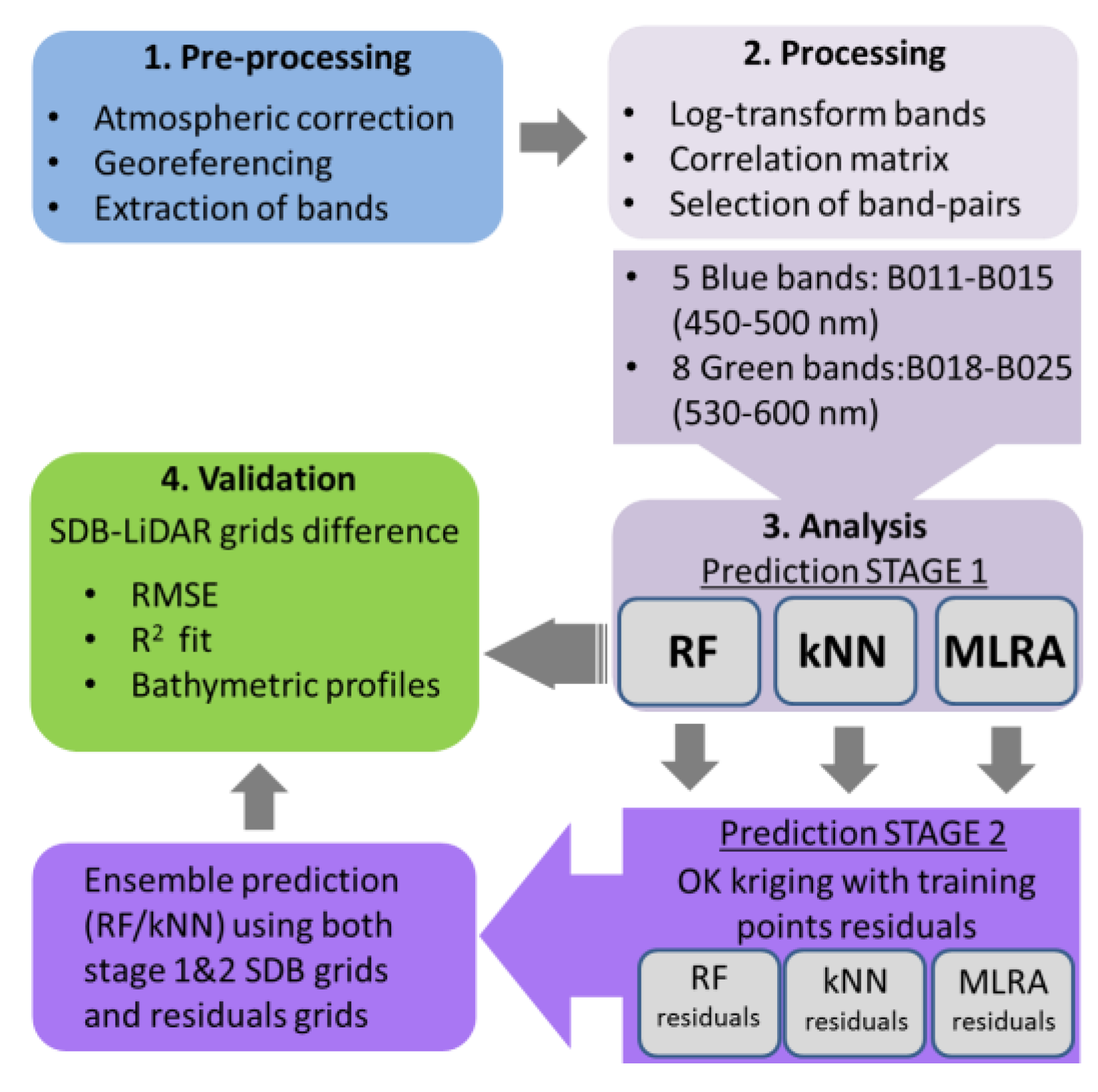
2. Materials and Methods
3. Results
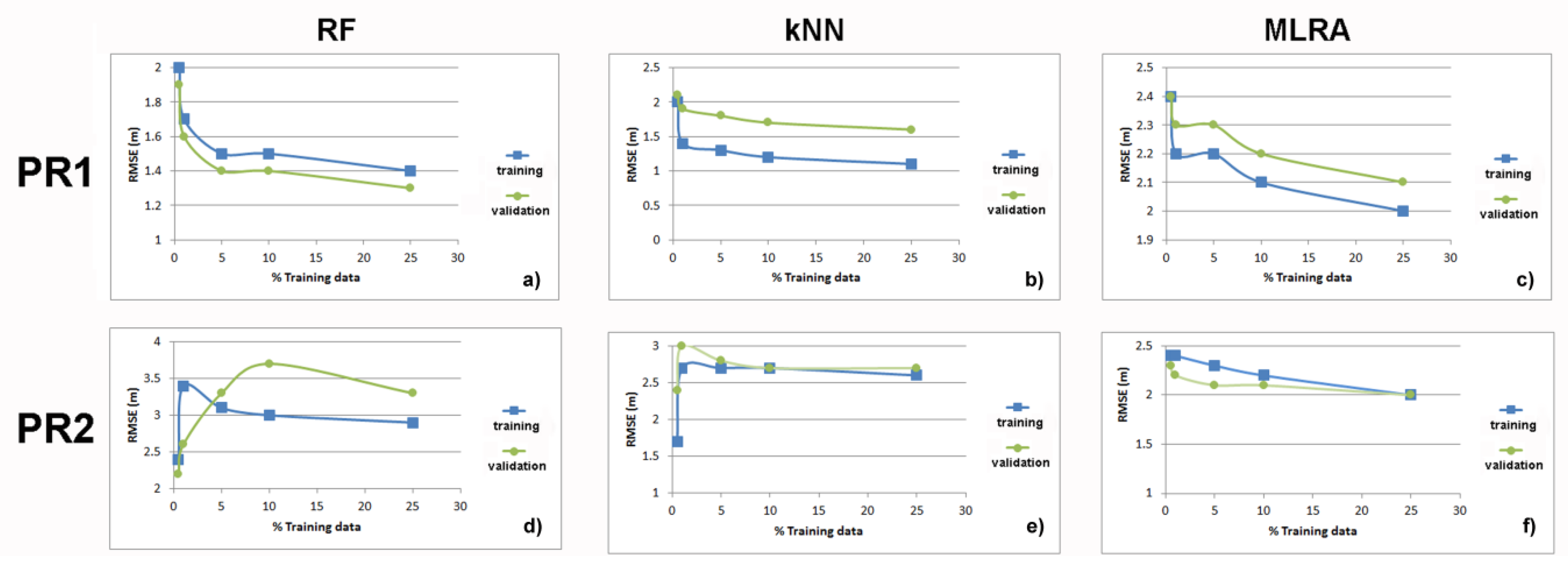
3.1. First Stage
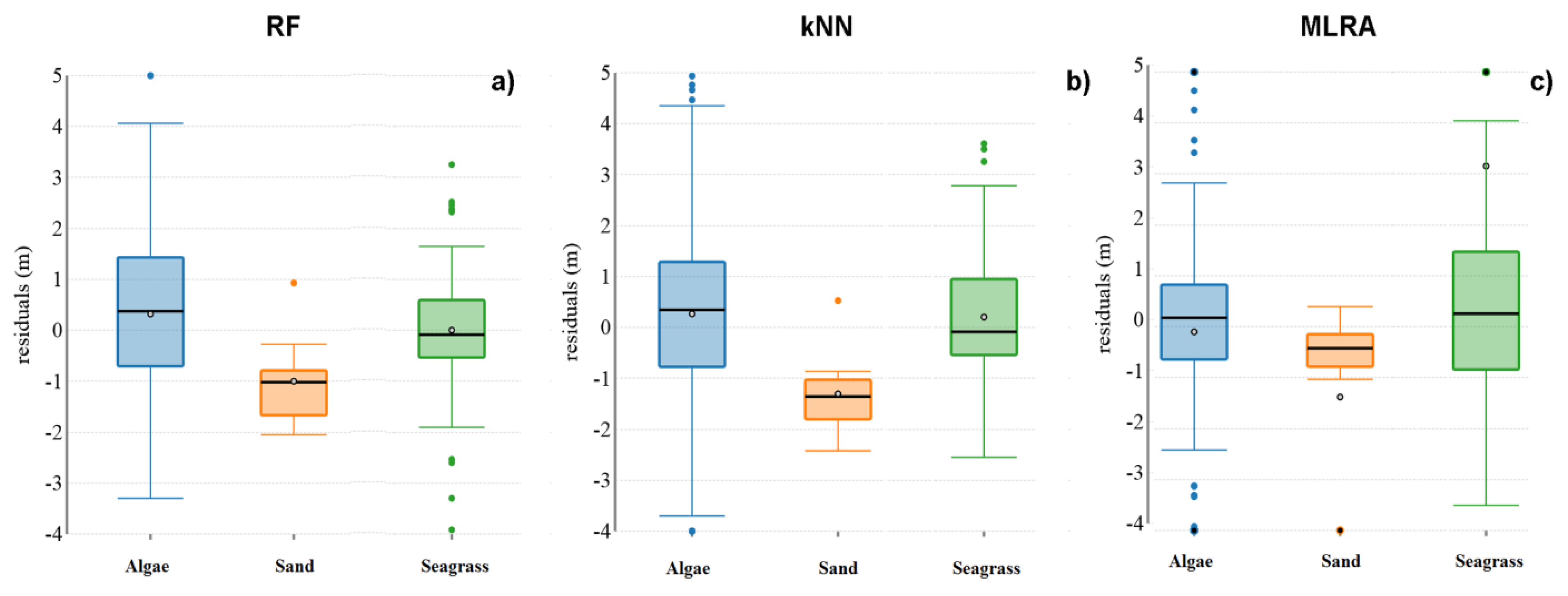
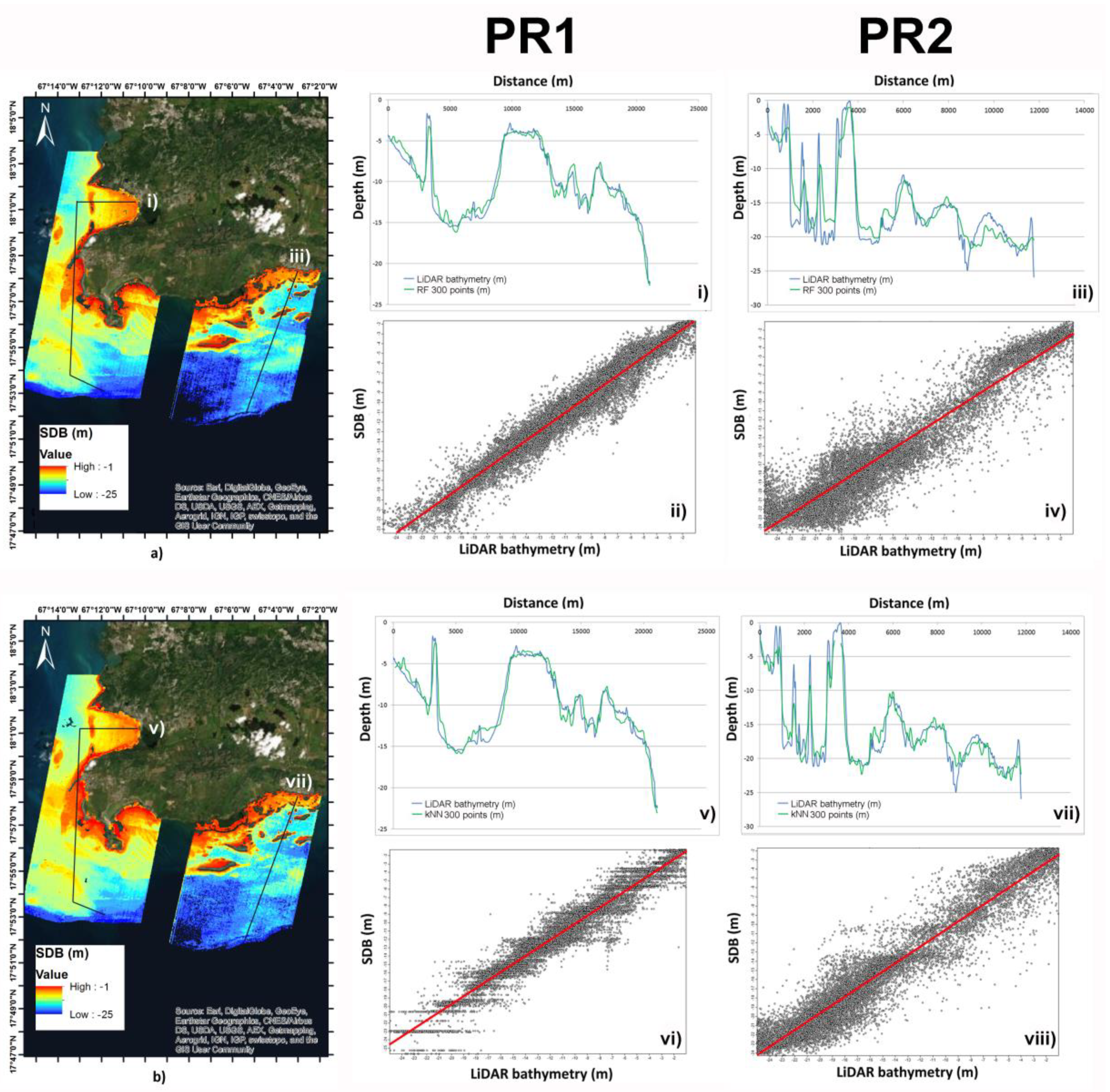
3.2. Second Stage
4. Discussion
4.1. Algorithm Performance
4.2. Comparison with Other SDB Methods Using Hyperspectral Imagery
5. Conclusions
Funding
Acknowledgments
Conflicts of Interest
Appendix A
References
- Wang, Y. Remote sensing of coastal environments. In Remote Sensing Applications; Taylor and Francis Series; CRC Press: Boca Raton, FL, USA, 2010; ISBN 978-1-42-009442-8. [Google Scholar]
- Hamylton, S. Hyperspectral remote sensing of the geomorphic features and habitats of the Al Wajh Bank reef systems, Saudi Arabia, Red Sea. In Seafloor Geomorphology as Benthic Habitat; Harris, P.T., Baker, E.K., Eds.; Elsevier: London, UK, 2012; pp. 357–365. [Google Scholar]
- Roelfsema, C.; Kovacs, E.; Ortiz, J.C.; Wolff, N.H.; Callaghan, D.; Wettle, M.; Ronan, M.; Hamylton, S.M.; Mumby, P.J.; Phinn, S. Coral reef habitat mapping: A combination of object-based image analysis and ecological modelling. Remote Sens. Environ. 2018, 208, 27–41. [Google Scholar] [CrossRef]
- El Mahrad, B.; Newton, A.; Icely, J.D.; Kacimi, I.; Abalansa, S.; Snoussi, M. Contribution of remote sensing technologies to a holistic coastal and marine environmental management framework: A review. Remote Sens. 2020, 12, 2313. [Google Scholar] [CrossRef]
- Li, R.; Liu, J.K.; Felus, Y. Spatial modeling and analysis for shoreline change detection and coastal erosion monitoring. Mar. Geod. 2001, 24, 1–12. [Google Scholar] [CrossRef]
- Lyzenga, D.R. Passive remote sensing techniques for mapping water depth and bottom features. Appl. Opt. 1978, 17, 379–383. [Google Scholar] [CrossRef] [PubMed]
- Stumpf, R.P.; Holderied, K.; Sinclair, M. Determination of water depth with high-resolution satellite imagery over variable bottom types. Limnol. Oceanogr. 2003, 48, 547–556. [Google Scholar] [CrossRef]
- Kutser, T.; Miller, I.; Jupp, D.L.B. Mapping coral reef benthic substrates using hyperspectral space-borne images and spectral libraries. Estuar. Coast. Shelf Sci. 2006, 70, 449–460. [Google Scholar] [CrossRef]
- Dekker, A.G.; Phinn, S.R.; Anstee, J.; Bissett, P.; Brando, V.E.; Casey, B.; Fearns, P.; Hedley, J.; Klonowski, W.; Lee, Z.P.; et al. Intercomparison of shallow water bathymetry, hydro-optics, and benthos mapping techniques in Australian and Caribbean coastal environments. Limnol. Oceanogr. Methods 2011, 9, 396–425. [Google Scholar] [CrossRef] [Green Version]
- Eugenio, F.; Marcello, J.; Martin, J. High-resolution maps of bathymetry and benthic habitats in shallow-water environments using multispectral remote sensing imager. IEEE Trans. Geosci. Rem. Sens. 2015, 53, 3539–3549. [Google Scholar] [CrossRef]
- Geyman, E.C.; Maloof, A.C. A simple method for extracting water depth from multispectral satellite imagery in regions of variable bottom type. Earth Space Sci. 2019, 6, 527–537. [Google Scholar] [CrossRef]
- Mavraeidopoulos, A.K.; Oikonomou, E.; Palikaris, A.; Poulos, S. A hybrid bio-optical transformation for satellite bathymetry modeling using sentinel-2 imagery. Remote Sens. 2019, 11, 2746. [Google Scholar] [CrossRef] [Green Version]
- Traganos, D.; Poursanidis, D.; Aggarwal, B.; Chrysoulakis, N.; Reinartz, P. Estimating satellite-derived bathymetry (SDB) with the Google Earth Engine and sentinel-2. Remote Sens. 2018, 10, 859. [Google Scholar] [CrossRef] [Green Version]
- Lyzenga, D.R. Shallow-water bathymetry using combined lidar and passive multispectral scanner data. Int. J. Remote Sens. 1985, 6, 115–125. [Google Scholar] [CrossRef]
- Dierssen, H.M.; Zimmerman, R.C.; Leathers, R.A.; Downes, T.V.; Davis, C.O. Ocean color remote sensing of seagrass and bathymetry in the Bahamas Banks by high-resolution airborne imagery. Limnol. Oceanogr. 2003, 48, 444–455. [Google Scholar] [CrossRef]
- Traganos, D.; Reinartz, P. Mapping Mediterranean seagrasses with Sentinel-2. Mar. Pollut. Bull. 2017, 134, 197–209. [Google Scholar] [CrossRef] [Green Version]
- Kobryn, H.T.; Wouters, K.; Beckley, L.E.; Heege, T. Ningaloo reef: Shallow marine habitats mapped using a hyperspectral sensor. PLoS ONE 2013, 8, e70105. [Google Scholar] [CrossRef] [Green Version]
- Gholamalifard, M.; Kutser, T.; Esmaili-Sari, A.; Abkar, A.A.; Naimi, B. Remotely sensed empirical modeling of bathymetry in the Southeastern Caspian Sea. Remote Sens. 2013, 5, 2746–2762. [Google Scholar] [CrossRef] [Green Version]
- Liu, S.; Gao, Y.; Zheng, W.; Li, X. Performance of two neural network models in bathymetry. Remote Sens. Lett. 2015, 6, 321–330. [Google Scholar] [CrossRef]
- Misra, A.; Vojinovic, Z.; Ramakrishnan, B.; Luijendijk, A.; Ranasinghe, R. Shallow water bathymetry mapping using Support Vector Machine (SVM) technique and multispectral imagery. Int. J. Remote Sens. 2018. [Google Scholar] [CrossRef]
- Wang, L.; Liu, H.; Su, H.; Wang, J. Bathymetry retrieval from optical images with spatially distributed support vector machines. GISci. Remote Sens. 2018. [Google Scholar] [CrossRef]
- McIntyre, M.L.; Naar, D.F.; Carder, K.L.; Donahue, B.T.; Mallinson, D.J. Coastal bathymetry from hyperspectral remote sensing data: Comparisons with high resolution multibeam bathymetry. Marine Geophys. Res. 2006, 27, 128–136. [Google Scholar] [CrossRef]
- Lee, Z.; Casey, B.; Arnone, R.; Weidemann, A.; Parsons, R.; Montes, M.J.; Gao, B.C.; Goode, W.; Davis, C.; Dye, J. Water and bottom properties of a coastal environment derived from Hyperion data measured from the EO-1 spacecraft platform. J. Appl. Remote Sens. 2007, 1, 011502. [Google Scholar]
- Johnson, L.J. The Underwater Optical Channel. 2012, pp. 1–18. Available online: https://www.researchgate.net/publication/280050464_The_Underwater_Optical_Channel/citation/download (accessed on 15 July 2020).
- Gomez, A.R. Spectral reflectance analysis of the Caribbean Sea. Geofís. Int. 2014, 53, 385–398. [Google Scholar] [CrossRef] [Green Version]
- NOAA, National Oceanic and Atmospheric Administration (NOAA). Digital Coast Data Access Viewer. Custom processing of 2006 NOAA Bathymetric Lidar: Puerto Rico; NOAA Office for Coastal Management: Charleston, SC, USA, 2006. Available online: https://coast.noaa.gov/dataviewer (accessed on 7 April 2020).
- Bauer, L.J.; Edwards, K.; Roberson, K.K.W.; Kendall, M.S.; Tormey, S.; Battista, T. Shallow-Water Benthic Habitats of Southwest Puerto Rico; NOAA Technical Memorandum NOAA NOS NCCOS 155: Silver Spring, MD, USA, 2012.
- Breiman, L. Random forests. Mach. Learn. 2001, 45, 5–32. [Google Scholar] [CrossRef] [Green Version]
- Diesing, M.; Green, S.L.; Stephens, D.; Lark, R.M.; Stewart, H.A.; Dove, D. Mapping seabed sediments: Comparison of manual, geostatistical, object-based image analysis and machine learning approaches. Cont. Shelf Res. 2014, 84, 107–119. [Google Scholar] [CrossRef] [Green Version]
- Zhang, C. Applying data fusion techniques for benthic habitat mapping and monitoring in a coral reef ecosystem. ISPRS J. Photogramm. Remote Sens. 2015, 104, 213–223. [Google Scholar] [CrossRef]
- Alevizos, E.; Greinert, J. The hyper-angular cube concept for improving the spatial and acoustic resolution of MBES backscatter angular response analysis. Geosciences 2018, 8, 446. [Google Scholar] [CrossRef] [Green Version]
- Sagawa, T.; Yamashita, Y.; Okumura, T.; Yamanokuchi, T. Satellite derived bathymetry using machine learning and multi-temporal satellite images. Remote Sens. 2019, 11, 1155. [Google Scholar] [CrossRef] [Green Version]
- King, R.D.; Feng, C.; Sutherland, A. Statlog: Comparison of classification algorithms on large real-world problems. Appl. Artif. Intell. 1995, 9, 289–333. [Google Scholar] [CrossRef]
- Imandoust, S.B.; Bolandraftar, M. Application of K-nearest neighbor (KNN) approach for predicting economic events: Theoretical background. Int. J. Eng. Res. Appl. 2013, 3, 605–610. [Google Scholar]
- Lucieer, V.; Hill, N.A.; Barrett, N.S.; Nichol, S. Do marine substrates ‘look’ and ‘sound’ the same? Supervised classification of multibeam acoustic data using autonomous underwater vehicle images. Estuar. Coast. Shelf Sci. 2013, 117, 94–106. [Google Scholar] [CrossRef]
- Lacharité, M.; Brown, C.J.; Gazzola, V. Multisource multibeam backscatter data: Developing a strategy for the production of benthic habitat maps using semi-automated seafloor classification methods. Mar. Geophys. Res. 2018, 39, 307–322. [Google Scholar] [CrossRef]
- Zelada Leon, A.; Huvenne, V.A.; Benoist, N.M.; Ferguson, M.; Bett, B.J.; Wynn, R.B. Assessing the repeatability of automated seafloor classification algorithms, with application in marine protected area monitoring. Remote Sens. 2020, 12, 1572. [Google Scholar] [CrossRef]
- Kibele, J.; Shears, N.T. Nonparametric empirical depth regression for bathymetric mapping in coastal waters. IEEE J. Sel. Top. Appl. Earth Obs. Remote Sens. 2016, 9, 5130–5138. [Google Scholar] [CrossRef]
- Bierwirth, P.; Burne, R.V. Shallow sea-floor reflectance and water depth derived by unmixing multispectral imagery. Photogramm. Eng. Remote Sens. 1993, 59, 331–338. [Google Scholar]
- Caballero, I.; Stump, P.R.; Meredith, A. Preliminary assessment of turbidity and chlorophyll impact on bathymetry derived from Sentinel-2A and Sentinel-3A satellites in South Florida. Remote Sens. 2019, 11, 645. [Google Scholar] [CrossRef] [Green Version]
- Lark, R.M.; Dove, D.; Green, S.L.; Richardson, A.E.; Stewart, H.; Stevenson, A. Spatial prediction of seabed sediment texture classes by cokriging from a legacy database of point observations. Sediment. Geol. 2012, 281, 35–49. [Google Scholar] [CrossRef] [Green Version]
- Conrad, O.; Bechtel, B.; Bock, M.; Dietrich, H.; Fischer, E.; Gerlitz, L.; Wehberg, J.; Wichmann, V.; Böhner, J. System for Automated Geoscientific Analyses (SAGA) v. 2.1.4. Geosci. Model Dev. 2015, 8, 1991–2007. [Google Scholar] [CrossRef] [Green Version]
- Ma, S.; Tao, Z.; Yang, X.; Yu, Y.; Zhou, X.; Li, Z. Bathymetry retrieval from hyperspectral remote sensing data in optical-shallow water. IEEE Trans. Geosci. Remote Sens. 2014, 52, 1205–1212. [Google Scholar] [CrossRef]
- Leiper, I.A.; Phinn, S.R.; Roelfsema, C.M.; Joyce, K.E.; Dekker, A.G. Mapping coral reef benthos, substrates, and bathymetry, using compact airborne spectrographic imager (CASI) data. Remote Sens. 2014, 6, 6423–6445. [Google Scholar] [CrossRef] [Green Version]
- Lyzenga, D.R.; Malinas, N.P.; Tanis, F.J. Multispectral bathymetry using a simple physically based algorithm. IEEE Trans. Geosci. Remote Sens. 2006, 44, 2251–2259. [Google Scholar] [CrossRef]


| Product Name | Acquisition Date/Time | Band Subset | Sub-Area |
|---|---|---|---|
| EO1H0050472011264110TE_1R | 21-Sep-2011/14:20 UTC | B011-B025 | PR1 |
| EO1H0050472013022110T5_1R | 22-Jan-2013/14:34 UTC | B011-B025 | PR2 |
| STAGE 1 | Predictors: Band Ratios | |||
|---|---|---|---|---|
| Area | Depth Range | RF | kNN | MLRA |
| PR1 | 0–25 m | RMSE: 1.9 m R2: 0.85 | RMSE: 2.1 m R2: 0.79 | RMSE: 2.4 m R2: 0.91 |
| PR2 | 0–25 m | RMSE: 2.3 m R2: 0.88 | RMSE: 2.4 m R2: 0.87 | RMSE: 2.2 m R2: 0.89 |
| STAGE 2 | Predictors: SDB from Stage 1 and Residuals | ||
|---|---|---|---|
| Area | Depth Range | RF | kNN |
| PR1 | 0–25 m | RMSE: 1.1 m R2: 0.95 | RMSE: 1.2 m R2: 0.94 |
| PR2 | 0–25 m | RMSE: 1.1 m R2: 0.89 | RMSE: 1.8 m R2: 0.92 |
Publisher’s Note: MDPI stays neutral with regard to jurisdictional claims in published maps and institutional affiliations. |
© 2020 by the author. Licensee MDPI, Basel, Switzerland. This article is an open access article distributed under the terms and conditions of the Creative Commons Attribution (CC BY) license (http://creativecommons.org/licenses/by/4.0/).
Share and Cite
Alevizos, E. A Combined Machine Learning and Residual Analysis Approach for Improved Retrieval of Shallow Bathymetry from Hyperspectral Imagery and Sparse Ground Truth Data. Remote Sens. 2020, 12, 3489. https://doi.org/10.3390/rs12213489
Alevizos E. A Combined Machine Learning and Residual Analysis Approach for Improved Retrieval of Shallow Bathymetry from Hyperspectral Imagery and Sparse Ground Truth Data. Remote Sensing. 2020; 12(21):3489. https://doi.org/10.3390/rs12213489
Chicago/Turabian StyleAlevizos, Evangelos. 2020. "A Combined Machine Learning and Residual Analysis Approach for Improved Retrieval of Shallow Bathymetry from Hyperspectral Imagery and Sparse Ground Truth Data" Remote Sensing 12, no. 21: 3489. https://doi.org/10.3390/rs12213489