Short-Term Forecasting of Satellite-Based Drought Indices Using Their Temporal Patterns and Numerical Model Output


Abstract
:
1. Introduction
2. Study Area and Data
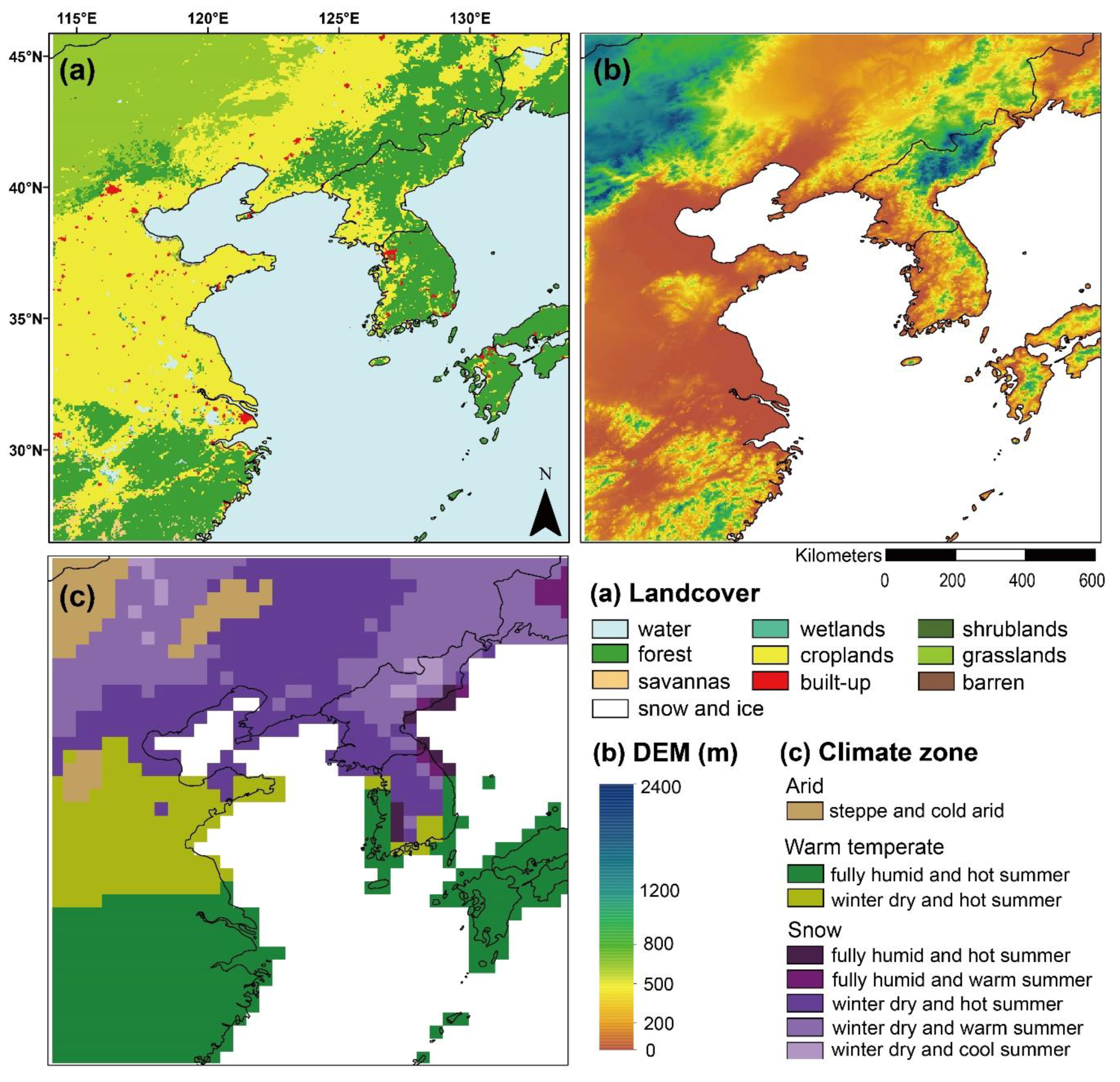
2.1. Study Area
2.2. Data
2.2.1. Satellite-Based Drought Indices
2.2.2. Numerical Model Outputs
2.2.3. Static Data
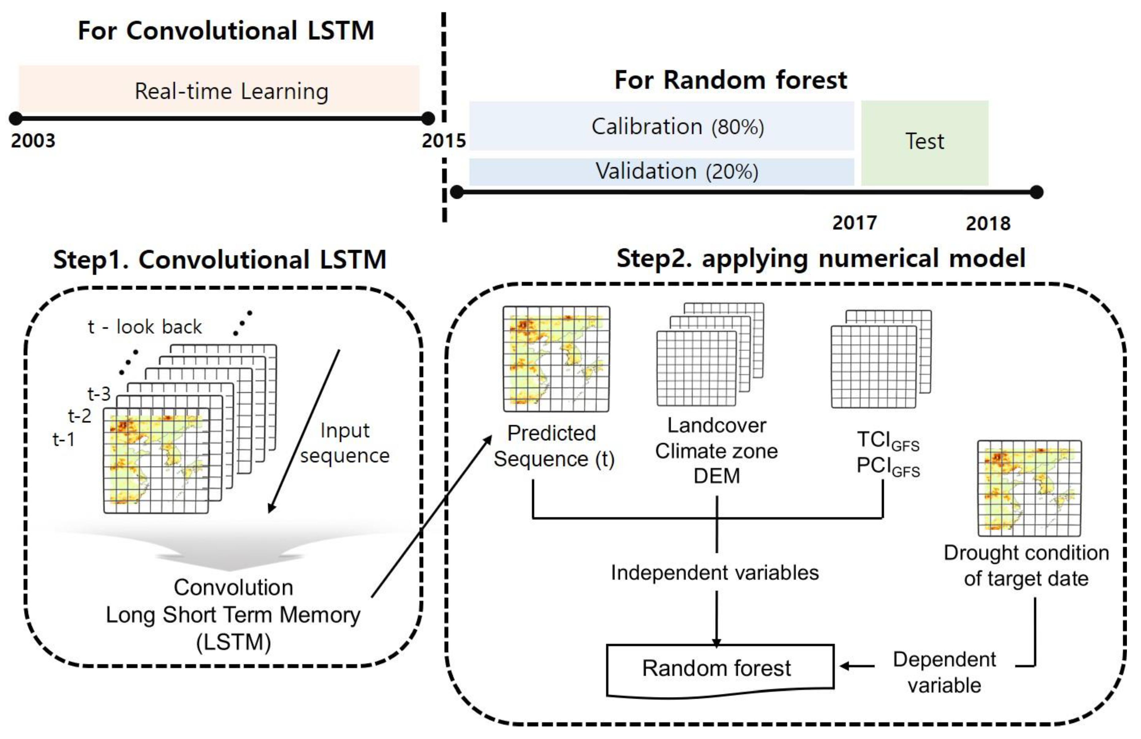
3. Methodology
3.1. Step 1: Convolutional Long Short Term Memory (ConvLSTM)
3.2. Step 2: Random Forest (RF)
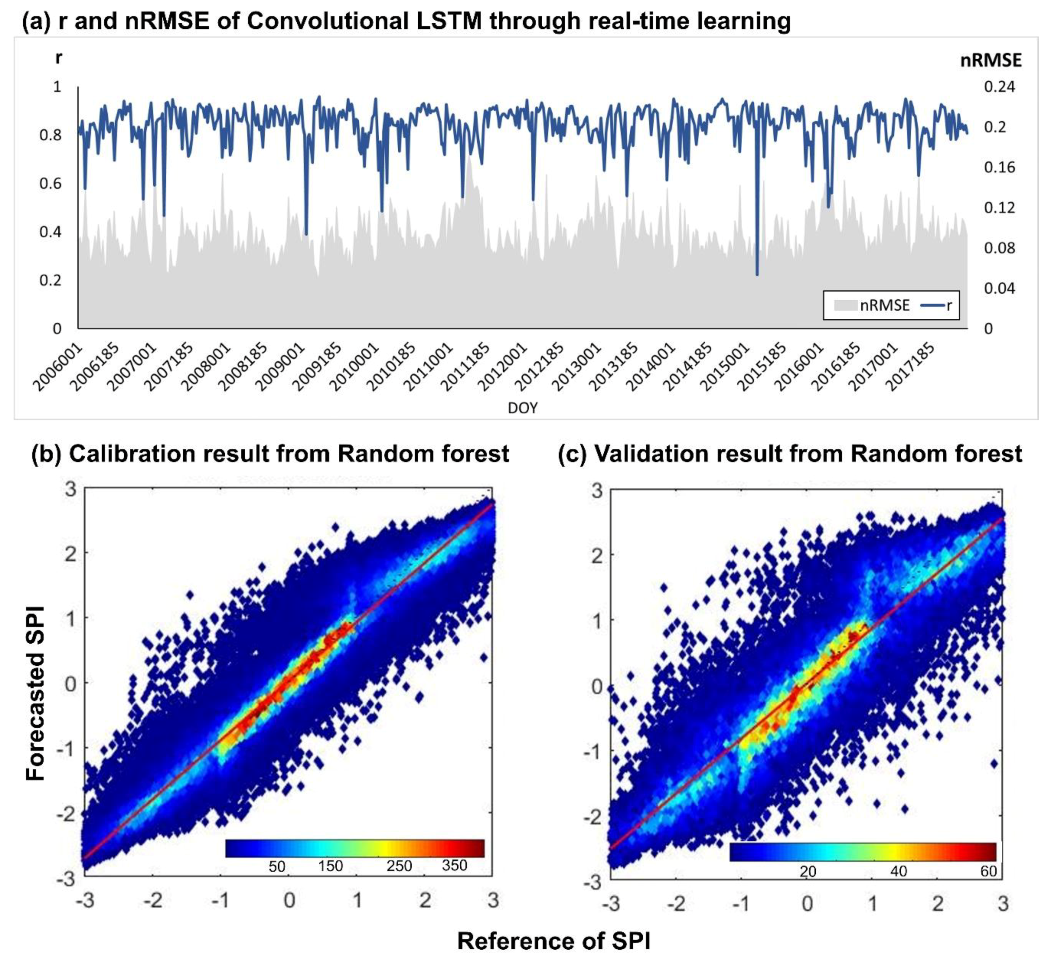
3.3. Accuracy Assessment
4. Results and Discussions
4.1. The Performance of Drought-Forecasting Model
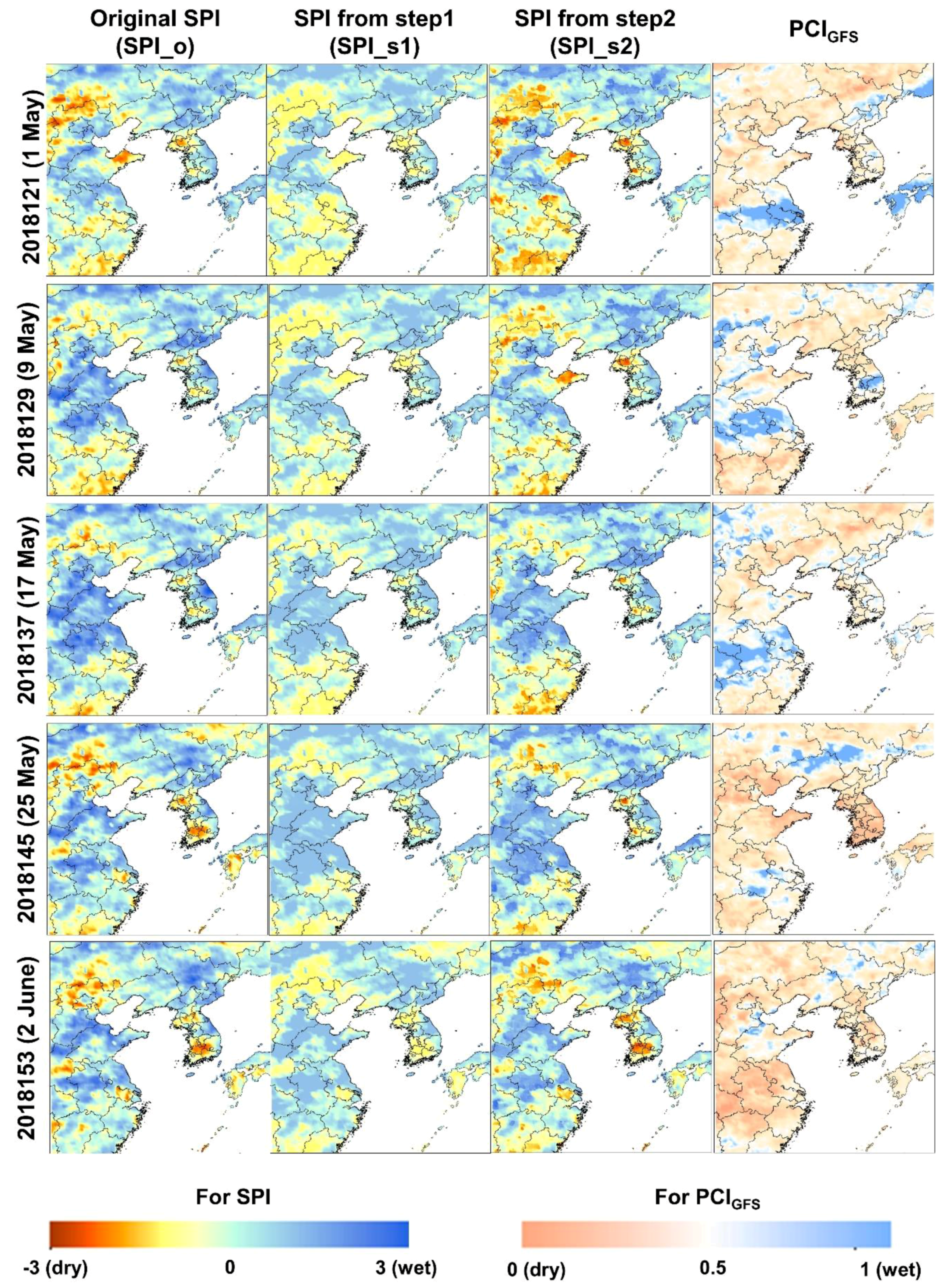
4.2. The Spatial Distribution of the Drought-Forecasting Model
4.3. Novelty and Limitations
5. Conclusions
Supplementary Materials
Author Contributions
Funding
Conflicts of Interest
References
- Sheffield, J.; Wood, E.F.; Chaney, N.; Guan, K.; Sadri, S.; Yuan, X.; Olang, L.; Amani, A.; Ali, A.; Demuth, S.; et al. A drought monitoring and forecasting system for sub-Sahara African water resources and food security. Bull. Am. Meteorol. Soc. 2014, 95, 861–882. [Google Scholar] [CrossRef]
- Bayissa, Y.A.; Tadesse, T.; Svoboda, M.; Wardlow, B.; Poulsen, C.; Swigart, J.; Van Andel, S.J. Developing a satellite-based combined drought indicator to monitor agricultural drought: A case study for Ethiopia. GISci. Remote Sens. 2019, 56, 718–748. [Google Scholar] [CrossRef]
- Han, L.; Zhang, Q.; Ma, P.; Jia, J.; Wang, J. The spatial distribution characteristics of a comprehensive drought risk index in southwestern China and underlying causes. Theor. Appl. Climatol. 2016, 124, 517–528. [Google Scholar] [CrossRef]
- NOAA National Centers for Environmental Information (NCEI) U.S. Billion-Dollar Weather and Climate Disasters. Available online: https://www.ncdc.noaa.gov/billions/ (accessed on 6 August 2020).
- Yan, H.; Moradkhani, H.; Zarekarizi, M. A probabilistic drought forecasting framework: A combined dynamical and statistical approach. J. Hydrol. 2017, 548, 291–304. [Google Scholar] [CrossRef] [Green Version]
- Tadesse, T.; Champagne, C.; Wardlow, B.D.; Hadwen, T.A.; Brown, J.F.; Demisse, G.B.; Bayissa, Y.A.; Davidson, A.M. Building the vegetation drought response index for Canada (VegDRI-Canada) to monitor agricultural drought: First results. GISci. Remote Sens. 2017, 54, 230–257. [Google Scholar] [CrossRef]
- Tran, H.T.; Campbell, J.B.; Tran, T.D.; Tran, H.T. Monitoring drought vulnerability using multispectral indices observed from sequential remote sensing (Case Study: Tuy Phong, Binh Thuan, Vietnam). GISci. Remote Sens. 2017, 54, 167–184. [Google Scholar] [CrossRef] [Green Version]
- Dai, A. Drought under global warming: A review. Wiley Interdiscip. Rev. Clim. Chang. 2011, 2, 45–65. [Google Scholar] [CrossRef] [Green Version]
- Dai, A. Increasing drought under global warming in observations and models. Nat. Clim. Chang. 2013, 3, 52–58. [Google Scholar] [CrossRef]
- Zhang, R.; Chen, Z.-Y.; Xu, L.-J.; Ou, C.-Q. Meteorological drought forecasting based on a statistical model with machine learning techniques in Shaanxi province, China. Sci. Total Environ. 2019, 665, 338–346. [Google Scholar] [CrossRef]
- Centre for Research on the Epidemiology of Disasters (CRED) Natural Disasters in 2018. 2019. Available online: https://cred.be/sites/default/files/adsr_2018.pdf (accessed on 6 August 2020).
- Belayneh, A.; Adamowski, J.; Khalil, B. Short-term SPI drought forecasting in the Awash River Basin in Ethiopia using wavelet transforms and machine learning methods. Sustain. Water Resour. Manag. 2016, 2, 87–101. [Google Scholar] [CrossRef]
- Demisse, G.B.; Tadesse, T.; Wall, N.; Haigh, T.; Bayissa, Y.; Shiferaw, A. Linking seasonal drought product information to decision makers in a data-sparse region: A case study in the Greater Horn of Africa. Remote Sens. Appl. Soc. Environ. 2019, 14, 200–206. [Google Scholar] [CrossRef]
- Rhee, J.; Im, J. Meteorological drought forecasting for ungauged areas based on machine learning: Using long-range climate forecast and remote sensing data. Agric. For. Meteorol. 2017, 237, 105–122. [Google Scholar] [CrossRef]
- Steinemann, A.C. Using climate forecasts for drought management. J. Appl. Meteorol. Climatol. 2006, 45, 1353–1361. [Google Scholar] [CrossRef]
- Climate Prediction Center (CPC). US Seasonal Drought Outlook (SDO). Available online: https://www.cpc.ncep.noaa.gov/products/outreach/publications.shtml (accessed on 6 August 2020).
- Mishra, A.K.; Singh, V.P. Drought modeling—A review. J. Hydrol. 2011, 403, 157–175. [Google Scholar] [CrossRef]
- Fung, K.F.; Huang, Y.F.; Koo, C.H.; Soh, Y.W. Drought forecasting: A review of modelling approaches 2007–2017. J. Water Clim. Chang. 2020, 11, 771–799. [Google Scholar] [CrossRef]
- Zargar, A.; Sadiq, R.; Naser, B.; Khan, F.I. A review of drought indices. Environ. Rev. 2011, 19, 333–349. [Google Scholar] [CrossRef]
- Lohani, V.K.; Loganathan, G.V.; Mostaghimi, S. Long-term analysis and short-term forecasting of dry spells by Palmer Drought Severity Index. Hydrol. Res. 1998, 29, 21–40. [Google Scholar] [CrossRef]
- Cancelliere, A.; Di Mauro, G.; Bonaccorso, B.; Rossi, G. Drought forecasting using the standardized precipitation index. Water Resour. Manag. 2007, 21, 801–819. [Google Scholar] [CrossRef]
- Kim, T.-W.; Valdés, J.B. Nonlinear model for drought forecasting based on a conjunction of wavelet transforms and neural networks. J. Hydrol. Eng. 2003, 8, 319–328. [Google Scholar] [CrossRef] [Green Version]
- Morid, S.; Smakhtin, V.; Bagherzadeh, K. Drought forecasting using artificial neural networks and time series of drought indices. Int. J. Climatol. A J. R. Meteorol. Soc. 2007, 27, 2103–2111. [Google Scholar] [CrossRef]
- Belayneh, A.; Adamowski, J.; Khalil, B.; Ozga-Zielinski, B. Long-term SPI drought forecasting in the Awash River Basin in Ethiopia using wavelet neural network and wavelet support vector regression models. J. Hydrol. 2014, 508, 418–429. [Google Scholar] [CrossRef]
- Jiao, W.; Tian, C.; Chang, Q.; Novick, K.A.; Wang, L. A new multi-sensor integrated index for drought monitoring. Agric. For. Meteorol. 2019, 268, 74–85. [Google Scholar] [CrossRef] [Green Version]
- Rhee, J.; Im, J.; Carbone, G.J. Monitoring agricultural drought for arid and humid regions using multi-sensor remote sensing data. Remote Sens. Environ. 2010, 114, 2875–2887. [Google Scholar] [CrossRef]
- Otkin, J.A.; Anderson, M.C.; Hain, C.; Svoboda, M. Using temporal changes in drought indices to generate probabilistic drought intensification forecasts. J. Hydrometeorol. 2015, 16, 88–105. [Google Scholar] [CrossRef]
- Park, H.; Kim, K. Prediction of severe drought area based on random forest: Using satellite image and topography data. Water 2019, 11, 705. [Google Scholar] [CrossRef] [Green Version]
- Park, S.; Seo, E.; Kang, D.; Im, J.; Lee, M.-I. Prediction of drought on pentad scale using remote sensing data and MJO index through random forest over East Asia. Remote Sens. 2018, 10, 1811. [Google Scholar] [CrossRef] [Green Version]
- Lorenz, D.J.; Otkin, J.A.; Svoboda, M.; Hain, C.R.; Zhong, Y. Forecasting rapid drought intensification using the Climate Forecast System (CFS). J. Geophys. Res. Atmos. 2018, 123, 8365–8373. [Google Scholar] [CrossRef]
- Otkin, J.A.; Anderson, M.C.; Hain, C.; Svoboda, M. Examining the relationship between drought development and rapid changes in the evaporative stress index. J. Hydrometeorol. 2014, 15, 938–956. [Google Scholar] [CrossRef]
- Lorenz, D.J.; Otkin, J.A.; Svoboda, M.; Hain, C.R.; Anderson, M.C.; Zhong, Y. Predicting the US Drought Monitor using precipitation, soil moisture, and evapotranspiration anomalies. Part II: Intraseasonal drought intensification forecasts. J. Hydrometeorol. 2017, 18, 1963–1982. [Google Scholar] [CrossRef]
- Meng, L.; Ford, T.; Guo, Y. Logistic regression analysis of drought persistence in East China. Int. J. Climatol. 2017, 37, 1444–1455. [Google Scholar] [CrossRef]
- Li, J.; Zhou, S.; Hu, R. Hydrological drought class transition using SPI and SRI time series by loglinear regression. Water Resour. Manag. 2016, 30, 669–684. [Google Scholar] [CrossRef]
- Han, P.; Wang, P.X.; Zhang, S.Y. Drought forecasting based on the remote sensing data using ARIMA models. Math. Comput. Model. 2010, 51, 1398–1403. [Google Scholar] [CrossRef]
- Han, P.; Wang, P.; Tian, M.; Zhang, S.; Liu, J.; Zhu, D. Application of the ARIMA models in drought forecasting using the standardized precipitation index. In Proceedings of the International Conference on Computer and Computing Technologies in Agriculture, Zhangjiajie, China, 19–21 October 2012; pp. 352–358. [Google Scholar]
- Özger, M.; Mishra, A.K.; Singh, V.P. Long lead time drought forecasting using a wavelet and fuzzy logic combination model: A case study in Texas. J. Hydrometeorol. 2012, 13, 284–297. [Google Scholar] [CrossRef]
- Borji, M.; Malekian, A.; Salajegheh, A.; Ghadimi, M. Multi-time-scale analysis of hydrological drought forecasting using support vector regression (SVR) and artificial neural networks (ANN). Arab. J. Geosci. 2016, 9, 725. [Google Scholar] [CrossRef]
- Abebe, A.; Foerch, G. Stochastic simulation of the severity of hydrological drought. Water Environ. J. 2008, 22, 2–10. [Google Scholar] [CrossRef]
- Modarres, R. Streamflow drought time series forecasting. Stoch. Environ. Res. Risk Assess. 2007, 21, 223–233. [Google Scholar] [CrossRef]
- Park, S.; Park, H.; Im, J.; Yoo, C.; Rhee, J.; Lee, B.; Kwon, C. Delineation of high resolution climate regions over the Korean Peninsula using machine learning approaches. PLoS ONE 2019, 14, e0223362. [Google Scholar] [CrossRef]
- Kottek, M.; Grieser, J.; Beck, C.; Rudolf, B.; Rubel, F. World map of the Köppen-Geiger climate classification updated. Meteorol. Zeitschrift 2006, 15, 259–263. [Google Scholar] [CrossRef]
- Han, Y.; Li, Z.; Huang, C.; Zhou, Y.; Zong, S.; Hao, T.; Niu, H.; Yao, H. Monitoring Droughts in the Greater Changbai Mountains Using Multiple Remote Sensing-Based Drought Indices. Remote Sens. 2020, 12, 530. [Google Scholar] [CrossRef] [Green Version]
- Kogan, F.N. Application of vegetation index and brightness temperature for drought detection. Adv. Sp. Res. 1995, 15, 91–100. [Google Scholar] [CrossRef]
- Kogan, F.N. Droughts of the late 1980s in the United States as derived from NOAA polar-orbiting satellite data. Bull. Am. Meteorol. Soc. 1995, 76, 655–668. [Google Scholar] [CrossRef] [Green Version]
- McKee, T.B.; Doesken, N.J.; Kleist, J. The relationship of drought frequency and duration to time scales. In Proceedings of the 8th Conference on Applied Climatology, Anaheim, CA, USA, 17–22 January 1993; Volume 17, pp. 179–183. [Google Scholar]
- Livada, I.; Assimakopoulos, V.D. Spatial and temporal analysis of drought in Greece using the Standardized Precipitation Index (SPI). Theor. Appl. Climatol. 2007, 89, 143–153. [Google Scholar] [CrossRef]
- Zhu, Q.; Luo, Y.; Zhou, D.; Xu, Y.-P.; Wang, G.; Gao, H. Drought monitoring utility using satellite-based precipitation products over the Xiang River Basin in China. Remote Sens. 2019, 11, 1483. [Google Scholar] [CrossRef] [Green Version]
- Tan, M.L.; Tan, K.C.; Chua, V.P.; Chan, N.W. Evaluation of TRMM product for monitoring drought in the Kelantan River Basin, Malaysia. Water 2017, 9, 57. [Google Scholar] [CrossRef] [Green Version]
- De Jesús, A.; Breña-Naranjo, J.A.; Pedrozo-Acuña, A.; Alcocer Yamanaka, V.H. The use of TRMM 3B42 product for drought monitoring in Mexico. Water 2016, 8, 325. [Google Scholar] [CrossRef]
- Yan, G.; Liu, Y.; Chen, X. Evaluating satellite-based precipitation products in monitoring drought events in southwest China. Int. J. Remote Sens. 2018, 39, 3186–3214. [Google Scholar] [CrossRef]
- Lee, T. Standardized Precipitation Index. Available online: https://www.mathworks.com/matlabcentral/fileexchange/26018-standardized-precipitation-index (accessed on 6 August 2020).
- Vogt, J.V.; Viau, A.A.; Paquet, F. Mapping regional air temperature fields using satellite-derived surface skin temperatures. Int. J. Climatol. A J. R. Meteorol. Soc. 1997, 17, 1559–1579. [Google Scholar] [CrossRef]
- Benali, A.; Carvalho, A.C.; Nunes, J.P.; Carvalhais, N.; Santos, A. Estimating air surface temperature in Portugal using MODIS LST data. Remote Sens. Environ. 2012, 124, 108–121. [Google Scholar] [CrossRef]
- He, K.; Sun, J. Convolutional neural networks at constrained time cost. In Proceedings of the IEEE Conference on Computer Vision and Pattern Recognition, Boston, MA, USA, 7–12 June 2015; pp. 5353–5360. [Google Scholar]
- Shi, X.; Chen, Z.; Wang, H.; Yeung, D.-Y.; Wong, W.-K.; Woo, W. Convolutional LSTM network: A machine learning approach for precipitation nowcasting. In Proceedings of the Advances in Neural Information Processing Systems, Montreal, QC, Canada, 7–12 December 2015; pp. 802–810. [Google Scholar]
- Ghimire, S.; Deo, R.C.; Raj, N.; Mi, J. Deep solar radiation forecasting with convolutional neural network and long short-term memory network algorithms. Appl. Energy 2019, 253, 113541. [Google Scholar] [CrossRef]
- Petrou, Z.I.; Tian, Y. Prediction of Sea Ice Motion With Convolutional Long Short-Term Memory Networks. IEEE Trans. Geosci. Remote Sens. 2019, 57, 6865–6876. [Google Scholar] [CrossRef]
- Song, A.; Choi, J.; Han, Y.; Kim, Y. Change detection in hyperspectral images using recurrent 3D fully convolutional networks. Remote Sens. 2018, 10, 1827. [Google Scholar] [CrossRef] [Green Version]
- Mu, B.; Peng, C.; Yuan, S.; Chen, L. ENSO Forecasting over Multiple Time Horizons Using ConvLSTM Network and Rolling Mechanism. In Proceedings of the 2019 International Joint Conference on Neural Networks (IJCNN), Shenzhen, China, 18–22 July 2019; pp. 1–8. [Google Scholar]
- Wen, C.; Liu, S.; Yao, X.; Peng, L.; Li, X.; Hu, Y.; Chi, T. A novel spatiotemporal convolutional long short-term neural network for air pollution prediction. Sci. Total Environ. 2019, 654, 1091–1099. [Google Scholar] [CrossRef] [PubMed]
- Mateo-Garcia, G.; Adsuara, J.E.; Pérez-Suay, A.; Gómez-Chova, L. Convolutional Long Short-Term Memory Network for Multitemporal Cloud Detection Over Landmarks. In Proceedings of the IGARSS 2019—2019 IEEE International Geoscience and Remote Sensing Symposium, Yokohama, Japan, 28 July–2 August 2019; pp. 210–213. [Google Scholar]
- Ma, C.; Li, S.; Wang, A.; Yang, J.; Chen, G. Altimeter Observation-Based Eddy Nowcasting Using an Improved Conv-LSTM Network. Remote Sens. 2019, 11, 783. [Google Scholar] [CrossRef] [Green Version]
- Cruz, G.; Bernardino, A. Learning Temporal Features for Detection on Maritime Airborne Video Sequences Using Convolutional LSTM. IEEE Trans. Geosci. Remote Sens. 2019, 57, 6565–6576. [Google Scholar] [CrossRef]
- Zhao, Z.; Wang, J.; Zhao, J.; Su, Z. Using a grey model optimized by differential evolution algorithm to forecast the per capita annual net income of rural households in China. Omega 2012, 40, 525–532. [Google Scholar] [CrossRef]
- Akay, D.; Atak, M. Grey prediction with rolling mechanism for electricity demand forecasting of Turkey. Energy 2007, 32, 1670–1675. [Google Scholar] [CrossRef]
- Kingma, D.P.; Ba, J. Adam: A method for stochastic optimization. arXiv 2014, arXiv:1412.6980. [Google Scholar]
- Breiman, L. Random forests. Mach. Learn. 2001, 45, 5–32. [Google Scholar] [CrossRef] [Green Version]
- Park, S.; Kim, D.-J.; Lee, S.-W.; Lee, K.-W.; Kim, J.; Song, E.-J.; Seo, K.-H. Comparison of extended medium-range forecast skill between KMA ensemble, ocean coupled ensemble, and GloSea5. Asia Pac. J. Atmos. Sci. 2017, 53, 393–401. [Google Scholar] [CrossRef]
- McLaren, K.; McIntyre, K.; Prospere, K. Using the random forest algorithm to integrate hydroacoustic data with satellite images to improve the mapping of shallow nearshore benthic features in a marine protected area in Jamaica. GISci. Remote Sens. 2019, 56, 1065–1092. [Google Scholar] [CrossRef]
- Jang, E.; Kang, Y.; Im, J.; Lee, D.-W.; Yoon, J.; Kim, S.-K. Detection and monitoring of forest fires using Himawari-8 geostationary satellite data in South Korea. Remote Sens. 2019, 11, 271. [Google Scholar] [CrossRef] [Green Version]
- Cho, D.; Yoo, C.; Im, J.; Lee, Y.; Lee, J. Improvement of spatial interpolation accuracy of daily maximum air temperature in urban areas using a stacking ensemble technique. GISci. Remote Sens. 2020, 57, 1–17. [Google Scholar] [CrossRef]
- Hyndman, R.J.; Koehler, A.B. Another look at measures of forecast accuracy. Int. J. Forecast. 2006, 22, 679–688. [Google Scholar] [CrossRef] [Green Version]
- Park, S.; Shin, M.; Im, J.; Song, C.-K.; Choi, M.; Kim, J.; Lee, S.; Park, R.; Kim, J.; Lee, D.-W.; et al. Estimation of ground-level particulate matter concentrations through the synergistic use of satellite observations and process-based models over South Korea. Atmos. Chem. Phys. 2019, 19, 1097–1113. [Google Scholar] [CrossRef] [Green Version]
- Park, S.; Im, J.; Jang, E.; Rhee, J. Drought assessment and monitoring through blending of multi-sensor indices using machine learning approaches for different climate regions. Agric. For. Meteorol. 2016, 216, 157–169. [Google Scholar] [CrossRef]
- Im, J.; Park, S.; Rhee, J.; Baik, J.; Choi, M. Downscaling of AMSR-E soil moisture with MODIS products using machine learning approaches. Environ. Earth Sci. 2016, 75, 1120. [Google Scholar] [CrossRef]
- Davydenko, A.; Fildes, R. Forecast error measures: Critical review and practical recommendations. In Business Forecasting: Practical Problems and Solutions; Wiley: New York, NY, USA, 2016; Volume 34. [Google Scholar]
- Choi, J.W.; Cha, Y.; Kim, J.Y. Prediction Experiment of Regional Drought over Korea Using the Similarity of Spatiotemporal Patterns of Past Droughts. J. Clim. Weather Forecast. 2017, 5, 2. [Google Scholar] [CrossRef] [Green Version]
- Kumar, P.; Kishtawal, C.M.; Pal, P.K. Skill of regional and global model forecast over Indian region. Theor. Appl. Climatol. 2016, 123, 629–636. [Google Scholar] [CrossRef]
- Lee, J.; Im, J.; Cha, D.-H.; Park, H.; Sim, S. Tropical cyclone intensity estimation using multi-dimensional convolutional neural networks from geostationary satellite data. Remote Sens. 2020, 12, 108. [Google Scholar] [CrossRef] [Green Version]
- Ye, W.; Cheng, J.; Yang, F.; Xu, Y. Two-Stream Convolutional Network for Improving Activity Recognition Using Convolutional Long Short-Term Memory Networks. IEEE Access 2019, 7, 67772–67780. [Google Scholar] [CrossRef]


| SDCI Value (unitless) | SDCI Category | SPI Value (unitless) | SPI Category |
|---|---|---|---|
| 0.0 to < 0.1 | Exceptional Drought | -2.0 and less | Extreme Drought |
| 0.1 to < 0.2 | Extreme Drought | -1.99 to < -1.5 | Severe Drought |
| 0.2 to < 0.3 | Severe Drought | -1.5 to < -1.0 | Moderate Drought |
| 0.3 to < 0.4 | Moderate Drought | -1.0 to < 0 | Mild Drought |
| 0.4 to < 0.5 | Abnormally Dry | 0 or more | No Drought |
| 0.5 to <= 1 | No Drought |
| Variables (Collected Period) | Products | Spatial Resolution | Temporal Resolution | |
|---|---|---|---|---|
| Drought indices (from 2003 to 2018) | SDCI | Terra MODIS Normalized Difference Vegetation Index (NDVI, MOD13C1) | 0.05° | 16 days |
| Terra MODIS Land Surface Temperature (LST, MOD11C2) | 8 days | |||
| SPI | TRMM precipitation (3B42) | 0.25° | daily | |
| Numerical model (from 2015 to 2018) | GFS air temperature | 0.5° | 3 h (to 240 h) | |
| GFS precipitation | ||||
| Static data | Terra MODIS landcover (MCD12C1) | 0.05° | yearly | |
| SRTM digital elevation model (DEM) | 90 m | - | ||
| Climate zone (Kottek et al. [42]) | 0.5° | |||
Publisher’s Note: MDPI stays neutral with regard to jurisdictional claims in published maps and institutional affiliations. |
© 2020 by the authors. Licensee MDPI, Basel, Switzerland. This article is an open access article distributed under the terms and conditions of the Creative Commons Attribution (CC BY) license (http://creativecommons.org/licenses/by/4.0/).
Share and Cite
Park, S.; Im, J.; Han, D.; Rhee, J. Short-Term Forecasting of Satellite-Based Drought Indices Using Their Temporal Patterns and Numerical Model Output. Remote Sens. 2020, 12, 3499. https://doi.org/10.3390/rs12213499
Park S, Im J, Han D, Rhee J. Short-Term Forecasting of Satellite-Based Drought Indices Using Their Temporal Patterns and Numerical Model Output. Remote Sensing. 2020; 12(21):3499. https://doi.org/10.3390/rs12213499
Chicago/Turabian StylePark, Sumin, Jungho Im, Daehyeon Han, and Jinyoung Rhee. 2020. "Short-Term Forecasting of Satellite-Based Drought Indices Using Their Temporal Patterns and Numerical Model Output" Remote Sensing 12, no. 21: 3499. https://doi.org/10.3390/rs12213499